This paper was converted on www.awesomepapers.org from LaTeX by an anonymous user.
Want to know more? Visit the Converter page.

A Revisit of The Energy Quadratization Method with A Relaxation Technique

Jia Zhao\comma\corrauth 1 11affiliationmark:  Department of Mathematics & Statistics, Utah State University, Logan, UT, USA [email protected]. (J. Zhao)
Abstract

This letter revisits the energy quadratization (EQ) method by introducing a novel and essential relaxation technique to improve its accuracy and stability. The EQ method has witnessed significant popularity in the past few years. Though acknowledging its effectiveness in designing energy-stable schemes for thermodynamically consistent models, the primary known drawback is apparent, i.e., its preserves a ”modified” energy law represented by auxiliary variables instead of the original variables. Truncation errors are introduced during numerical calculations so that the numerical solutions of the auxiliary variables are no longer equivalent to their original continuous definitions. Even though the ”modified” energy dissipation law is preserved, the original energy dissipation law is not guaranteed. In this paper, we overcome this issue by introducing a relaxation technique. The computational cost of this extra technique is negligible compared with the baseline EQ method. Meanwhile, the relaxed-EQ method holds all the baseline EQ method’s good properties, such as linearity and unconditionally energy stability. Then we apply the relaxed-EQ method to several widely-used phase field models to highlight its effectiveness.

keywords:
Energy Quadratization (EQ); Energy Stable; Phase Field Models; Onsager Principle
\ams

1 Background

In this letter, we focus on the PDE models that respect the thermodynamical laws. They are usually named thermodynamically consistent models. In particular, when the temperature deviation is considered, the PDE model’s entropy shall be non-decreasing in time. When the temperature deviation is ignored, the PDE model’s Helmholtz free energy shall be non-increasing in time. These thermodynamically consistent models are broadly used to investigate problems in various fields, taking material science, life science, and mechanical engineering as examples.

In the past few decades, a community is shaped on developing numerical algorithms to solve the thermodynamically consistent models while preserving their thermodynamical structures [8, 6, 3, 7, 4]. Among many seminal publications, the energy quadratization (EQ) method has witnessed an intense exploration [9, 10, 2].

To illustrate the idea of the EQ method, we start with a simple example, the Allen-Cahn (AC) equation with periodic boundary condition, given as

tϕ(𝐱,t)=ε2Δϕ(𝐱,t)ϕ(𝐱,t)3+ϕ(𝐱,t),(𝐱,t)Ω×(0,T].\partial_{t}\phi(\mathbf{x},t)=\varepsilon^{2}\Delta\phi(\mathbf{x},t)-\phi(\mathbf{x},t)^{3}+\phi(\mathbf{x},t),\quad(\mathbf{x},t)\in\Omega\times(0,T]. (1.1)

Define the free energy

F=Ωε22|ϕ|2+14(ϕ21)2d𝐱,F=\int_{\Omega}\frac{\varepsilon^{2}}{2}|\nabla\phi|^{2}+\frac{1}{4}(\phi^{2}-1)^{2}d\mathbf{x},

with ε\varepsilon a model parameter. It is known that the AC equation in (1.1) satisfies the energy dissipation law

dFdt=ΩδFδϕϕt𝑑𝐱=Ω(ϕt)2𝑑𝐱0.\frac{dF}{dt}=\int_{\Omega}\frac{\delta F}{\delta\phi}\frac{\partial\phi}{\partial t}d\mathbf{x}=-\int_{\Omega}(\frac{\partial\phi}{\partial t})^{2}d\mathbf{x}\leq 0. (1.2)

To design numerical schemes that preserve the energy dissipation law for the AC equation, the EQ method introduces a novel perspective, namely, instead of solving the original AC equation in (1.1), it solves an equivalent problem. By introducing the auxiliary variable

q(𝐱,t):=h(ϕ)=22(ϕ21),q(\mathbf{x},t):=h(\phi)=\frac{\sqrt{2}}{2}(\phi^{2}-1),

and the notation g(ϕ):=qϕ=2ϕg(\phi):=\frac{\partial q}{\partial\phi}=\sqrt{2}\phi, the equivalent problem is formulated as

tϕ=ε2Δϕ(𝐱,t)qg(ϕ),\displaystyle\partial_{t}\phi=\varepsilon^{2}\Delta\phi(\mathbf{x},t)-qg(\phi), (1.3a)
tq=g(ϕ)tϕ,\displaystyle\partial_{t}q=g(\phi)\partial_{t}\phi, (1.3b)

with consistent initial condition q|t=0=22(ϕ2|t=01)q|_{t=0}=\frac{\sqrt{2}}{2}(\phi^{2}|_{t=0}-1). The reformulated problem has an equivalent energy dissipation law

dEdt=ΩδEδϕϕt+δEδqqtd𝐱=Ω(ϕt)2𝑑𝐱0,\frac{dE}{dt}=\int_{\Omega}\frac{\delta E}{\delta\phi}\frac{\partial\phi}{\partial t}+\frac{\delta E}{\delta q}\frac{\partial q}{\partial t}d\mathbf{x}=-\int_{\Omega}(\frac{\partial\phi}{\partial t})^{2}d\mathbf{x}\leq 0, (1.4)

where the modified free energy is defined as E=Ωε22|ϕ|2+12q2d𝐱.E=\int_{\Omega}\frac{\varepsilon^{2}}{2}|\nabla\phi|^{2}+\frac{1}{2}q^{2}d\mathbf{x}. In the PDE level, it is known that q=h(ϕ)=22(ϕ21)q=h(\phi)=\frac{\sqrt{2}}{2}(\phi^{2}-1), so that the reformulated problem in (1.3) is equivalent with (1.1), as well as their energy dissipation laws.

However, the numerical solutions for qq and the numerical results of h(ϕ)h(\phi) are not necessarily equal any more (in fact, they are not) after temporal discretization. Hence a discrete energy dissipation law in (1.4) is no longer equivalent with a discrete energy dissipation law in (1.2), though we shall recognize that they are consistent with the numerical schemes’ order of temporal accuracy.

With this in mind, the primary goal of this letter is to overcome this inconsistency issue. And our central idea is to introduce a relaxation technique for the numerical solutions of qq, to penalize the numerical deviation from the original definition of q:=h(ϕ)q:=h(\phi).

2 Thermodynamically consistent reversible-irreversible PDE models

2.1 A generic model formulation

Consider a domain Ω\Omega, and denote the thermodynamic variable as ϕ\phi. We introduce the general formulation for a thermodynamically consistent reversible-irreversible PDE models as

tϕ(𝐱,t)=𝒢δδϕ in Ω,\displaystyle\partial_{t}\phi(\mathbf{x},t)=-\mathcal{G}\frac{\delta\mathcal{E}}{\delta\phi}\mbox{ in }\Omega, (2.1a)
(ϕ(𝐱,t))=g(𝐱,t), on Ω,\displaystyle\mathcal{B}(\phi(\mathbf{x},t))=g(\mathbf{x},t),\mbox{ on }\partial\Omega, (2.1b)

where \mathcal{B} is a trace operator, and 𝒢:=𝒢a+𝒢s\mathcal{G}:=\mathcal{G}_{a}+\mathcal{G}_{s} is the mobility operator, 𝒢s\mathcal{G}_{s} is symmetric and positive semi-definite to ensure thermodynamically consistency, 𝒢a\mathcal{G}_{a} is skew-symmetric, and δδϕ\frac{\delta\mathcal{E}}{\delta\phi} is the variational derivative of \mathcal{E}, known as the chemical potential. Then, the triplet (ϕ,𝒢,)(\phi,\mathcal{G},\mathcal{E}) uniquely defines a thermodynamically consistent model. One intrinsic property of (2.1) owing to the thermodynamical consistency is the energy dissipation law

ddt=(δδϕ,ϕt)+˙surf=˙bulk+˙surf,\displaystyle\frac{d\mathcal{E}}{dt}=\Big{(}\frac{\delta\mathcal{E}}{\delta\phi},\frac{\partial\phi}{\partial t}\Big{)}+\dot{\mathcal{E}}_{surf}=\dot{\mathcal{E}}_{bulk}+\dot{\mathcal{E}}_{surf}, (2.2a)
˙bulk=(δδϕ,𝒢sδFδϕ)0,(δδϕ,𝒢aδδϕ)=0,˙surf=Ωgb𝑑s,\displaystyle\dot{\mathcal{E}}_{bulk}=-\Big{(}\frac{\delta\mathcal{E}}{\delta\phi},\mathcal{G}_{s}\frac{\delta F}{\delta\phi}\Big{)}\leq 0,\quad\Big{(}\frac{\delta\mathcal{E}}{\delta\phi},\mathcal{G}_{a}\frac{\delta\mathcal{E}}{\delta\phi}\Big{)}=0,\quad\dot{\mathcal{E}}_{surf}=\int_{\partial\Omega}g_{b}ds, (2.2b)

where the inner product is defined by (f,g)=Ωfg𝑑𝐱(f,g)=\int_{\Omega}fgd\mathbf{x},f,gL2(Ω)\forall f,g\in L^{2}(\Omega), and ˙surf\dot{\mathcal{E}}_{surf} is due to the boundary contribution, and gbg_{b} is the boundary integrand. When 𝒢a=0\mathcal{G}_{a}=0, (2.1) is a purely dissipative system; while 𝒢s=0\mathcal{G}_{s}=0, it is a purely dispersive system. ˙surf\dot{\mathcal{E}}_{surf} vanishes only for suitable boundary conditions, which include periodic and certain physical boundary conditions.

2.2 Model reformulation with the energy quadratization method

Now, we illustrate the energy quadratization (EQ) idea on solving (2.1). Denote the total energy as (ϕ)=Ωe𝑑𝐱\mathcal{E}(\phi)=\int_{\Omega}ed\mathbf{x}, with ee the energy density function. We denote L0L_{0} as a linear operator that can be separated from ee. Introduce the auxiliary variable

q=:h(ϕ)=2(e12|012ϕ|2+A0|Ω|),q=:h(\phi)=\sqrt{2\Big{(}e-\frac{1}{2}|\mathcal{L}_{0}^{\frac{1}{2}}\phi|^{2}+\frac{A_{0}}{|\Omega|}\Big{)}}, (2.3)

where A0>0A_{0}>0 such that qq is a well defined real variable. Then we rewrite the energy as

(ϕ,q)=12(ϕ,0ϕ)+12(q,q)A0,\mathcal{E}(\phi,q)=\frac{1}{2}\Big{(}\phi,\mathcal{L}_{0}\phi\Big{)}+\frac{1}{2}\Big{(}q,q\Big{)}-A_{0}, (2.4)

With the EQ approach above, we transform the free energy density into a quadratic one by introducing an auxiliary variable to ”remove” the quadratic gradient term from the energy density. Assuming q=q(ϕ,ϕ)q=q(\phi,\nabla\phi) and denoting g(ϕ)=qϕg(\phi)=\frac{\partial q}{\partial\phi} and 𝐆(ϕ)=qϕ\mathbf{G}(\nabla\phi)=\frac{\partial q}{\partial\nabla\phi}, we reformulate (2.1) into an equivalent form

tϕ=(𝒢a+𝒢s)[0ϕ+qg(ϕ)(q𝐆(ϕ))],\displaystyle\partial_{t}\phi=-(\mathcal{G}_{a}+\mathcal{G}_{s})\Big{[}\mathcal{L}_{0}\phi+qg(\phi)-\nabla\cdot(q\mathbf{G}(\nabla\phi))\Big{]}, (2.5a)
tq=g(ϕ):tϕ+𝐆(ϕ):tϕ,\displaystyle\partial_{t}q=g(\phi):\partial_{t}\phi+\mathbf{G}(\nabla\phi):\nabla\partial_{t}\phi, (2.5b)

with the consistent initial condition q|t=0=2(e12|012ϕ|2+A0|Ω|)|t=0q|_{t=0}=\left.\sqrt{2\Big{(}e-\frac{1}{2}|\mathcal{L}_{0}^{\frac{1}{2}}\phi|^{2}+\frac{A_{0}}{|\Omega|}\Big{)}}\right|_{t=0}. Now, instead of dealing with (2.1) directly, we develop structure-preserving schemes for (2.5).

The advantage of using model (2.5) over model (2.1) is that the energy density is transformed into a quadratic one in (2.5). Denoting Ψ=[ϕq]\Psi=\begin{bmatrix}\phi\\ q\end{bmatrix}, we rewrite (2.5) into a compact from

tΨ=𝒩(Ψ)Ψ,\partial_{t}\Psi=-\mathcal{N}(\Psi)\mathcal{L}\Psi, (2.6)

where \mathcal{L} is a linear operator, and 𝒩(Ψ)\mathcal{N}(\Psi) is the mobility operator as

𝒩(Ψ)=𝒩s(Ψ)+𝒩a(Ψ),𝒩a(Ψ)=𝒩0𝒢a𝒩0,𝒩s(Ψ)=𝒩0𝒢s𝒩0.\mathcal{N}(\Psi)=\mathcal{N}_{s}(\Psi)+\mathcal{N}_{a}(\Psi),\quad\mathcal{N}_{a}(\Psi)=\mathcal{N}_{0}^{\ast}\mathcal{G}_{a}\mathcal{N}_{0},\quad\mathcal{N}_{s}(\Psi)=\mathcal{N}_{0}^{\ast}\mathcal{G}_{s}\mathcal{N}_{0}. (2.7)

Here 𝒩0=(1,g(ϕ)+𝐆(ϕ):)\mathcal{N}_{0}=(1,\,\,\,g(\phi)+\mathbf{G}(\nabla\phi)\colon\nabla), =[01],\mathcal{L}=\begin{bmatrix}\mathcal{L}_{0}&\\ &1\end{bmatrix}, and 𝒩0\mathcal{N}_{0}^{\ast} is the adjoint operator of 𝒩0\mathcal{N}_{0}. When ˙surf=0\dot{\mathcal{E}}_{surf}=0, the energy law is

d(Ψ)dt=(δδΨdΨdt,1)=(Ψ,𝒩(Ψ)Ψ)=(𝒩0Ψ,𝒢s𝒩0Ψ)0.\frac{d\mathcal{E}(\Psi)}{dt}=\Big{(}\frac{\delta\mathcal{E}}{\delta\Psi}\frac{d\Psi}{dt},1\Big{)}=-\Big{(}\ \mathcal{L}\Psi,\mathcal{N}(\Psi)\mathcal{L}\Psi\Big{)}=-\Big{(}\mathcal{N}_{0}\mathcal{L}\Psi,\mathcal{G}_{s}\mathcal{N}_{0}\mathcal{L}\Psi\Big{)}\leq 0. (2.8)

2.3 Model examples

To demonstrate this methodology’s generality, we introduce a few widely-used PDE models that can be cast as special cases.

Allen Cahn equation. First of all, let us consider the Allen-Cahn equation

tϕ=ε2Δϕϕ3+ϕ.\partial_{t}\phi=\varepsilon^{2}\Delta\phi-\phi^{3}+\phi. (2.9)

It can be formulated in an energy variation form of (2.1) with 𝒢=1\mathcal{G}=1 and F=Ωε22|ϕ|2+14(ϕ21)2d𝐱F=\int_{\Omega}\frac{\varepsilon^{2}}{2}|\nabla\phi|^{2}+\frac{1}{4}(\phi^{2}-1)^{2}d\mathbf{x}. Next, if we introduce q:=h(ϕ)=12(ϕ21γ0)q:=h(\phi)=\frac{1}{\sqrt{2}}(\phi^{2}-1-\gamma_{0}), we will have g(ϕ):=qϕ=2ϕg(\phi):=\frac{\partial q}{\partial\phi}=\sqrt{2}\phi. Then the model is reformulated into the quadratization form of (2.5) as

tϕ=ε2Δϕγ0ϕg(ϕ)q,\displaystyle\partial_{t}\phi=\varepsilon^{2}\Delta\phi-\gamma_{0}\phi-g(\phi)q, (2.10a)
tq=g(ϕ)tϕ,\displaystyle\partial_{t}q=g(\phi)\partial_{t}\phi, (2.10b)

with the consistent initial condition q|t=0=h(ϕ|t=0)q|_{t=0}=h(\phi|_{t=0}). Its matrix formulation of (2.6) can also be easily obtained, by noticing 0=ε2Δ+γ0\mathcal{L}_{0}=-\varepsilon^{2}\Delta+\gamma_{0}.

Cahn-Hilliard (CH) equation. In the second example, we consider the Cahn-Hilliard equation given as

tϕ=MΔμ,\displaystyle\partial_{t}\phi=M\Delta\mu, (2.11a)
μ=ε2Δϕ+f(ϕ),\displaystyle\mu=-\varepsilon^{2}\Delta\phi+f^{\prime}(\phi), (2.11b)

where f(ϕ)f(\phi) is the bulk potential. In this paper, we choose the double-well potential f(ϕ)=14(ϕ21)2f(\phi)=\frac{1}{4}(\phi^{2}-1)^{2}. Other potentials, such as the Flory-Huggins potential can also be used. It can be reformulated in an energy variational form of (2.1) with the notations 𝒢=Δ\mathcal{G}=-\Delta, and F=Ω[ε22|ϕ|2+f(ϕ)]𝑑𝐱F=\int_{\Omega}\Big{[}\frac{\varepsilon^{2}}{2}|\nabla\phi|^{2}+f(\phi)\Big{]}d\mathbf{x}. Then, we introduce q:=h(ϕ)=12(ϕ21γ0)q:=h(\phi)=\frac{1}{\sqrt{2}}(\phi^{2}-1-\gamma_{0}) and g(ϕ):=qϕ=2ϕg(\phi):=\frac{\partial q}{\partial\phi}=\sqrt{2}\phi, leading us to the quadratized form of (2.5) as

tϕ=Δ(ε2ϕ+γ0ϕg(ϕ)q),\displaystyle\partial_{t}\phi=\Delta(-\varepsilon^{2}\phi+\gamma_{0}\phi-g(\phi)q), (2.12a)
tq=g(ϕ)tϕ,\displaystyle\partial_{t}q=g(\phi)\partial_{t}\phi, (2.12b)

with the consistent initial condition q|t=0=h(ϕ|t=0)q|_{t=0}=h(\phi|_{t=0}).

Molecular beam epitaxy (MBE) model. Then, we focus on the molecular beam epitaxy (MBE) model with slope section. The model reads

tϕ=M[ε2Δϕ2((|ϕ|21)ϕ)].\partial_{t}\phi=-M\Big{[}\varepsilon^{2}\Delta\phi^{2}-\nabla\cdot((|\nabla\phi|^{2}-1)\nabla\phi)\Big{]}. (2.13)

Similarly, this model can be written in an energy variation form of (2.1) as 𝒢=M\mathcal{G}=M and F=Ω[ε22(Δϕ)2+14(|ϕ|21)2]𝑑𝐱F=\int_{\Omega}\Big{[}\frac{\varepsilon^{2}}{2}(\Delta\phi)^{2}+\frac{1}{4}(|\nabla\phi|^{2}-1)^{2}\Big{]}d\mathbf{x}. If we introduce the notations q:=h(ϕ)=22(|ϕ|21γ0)q:=h(\phi)=\frac{\sqrt{2}}{2}(|\nabla\phi|^{2}-1-\gamma_{0}), and 𝐆(ϕ):=qϕ=2ϕ\mathbf{G}(\nabla\phi):=\frac{\partial q}{\partial\nabla\phi}=\sqrt{2}\nabla\phi, the MBE model can be written in the quadratized form as

tϕ=M[ε2Δ2ϕγΔϕ(q𝐆(ϕ))],\displaystyle\partial_{t}\phi=-M\Big{[}\varepsilon^{2}\Delta^{2}\phi-\gamma\Delta\phi-\nabla\cdot(q\mathbf{G}(\nabla\phi))\Big{]}, (2.14a)
tq=𝐆(ϕ):tϕ,\displaystyle\partial_{t}q=\mathbf{G}(\nabla\phi):\nabla\partial_{t}\phi, (2.14b)

with a consistent initial condition for qq.

Phase field crystal (PFC) equation. Next, we investigate the phase field crystal (PFC) equation which reads as

tϕ=Δ((a0+Δ)2ϕ+f(ϕ)),f(ϕ)=14ϕ4b02ϕ2,\partial_{t}\phi=\Delta((a_{0}+\Delta)^{2}\phi+f^{\prime}(\phi)),\quad f(\phi)=\frac{1}{4}\phi^{4}-\frac{b_{0}}{2}\phi^{2}, (2.15)

with a0a_{0} and b0b_{0} are model parameters. The PFC model can also be written in an energy variational form of (2.1) with 𝒢=Δ\mathcal{G}=\Delta , and F=Ω{12ϕ[b0+(a0+Δ)2]ϕ+14ϕ4}𝑑𝐱F=\int_{\Omega}\Big{\{}\frac{1}{2}\phi\Big{[}-b_{0}+(a_{0}+\Delta)^{2}\Big{]}\phi+\frac{1}{4}\phi^{4}\Big{\}}d\mathbf{x}. Then, if we introduce the notations q:=h(ϕ)=214ϕ4b02ϕ2γ02ϕ2+C0q:=h(\phi)=\sqrt{2}\sqrt{\frac{1}{4}\phi^{4}-\frac{b_{0}}{2}\phi^{2}-\frac{\gamma_{0}}{2}\phi^{2}+C_{0}} and g(ϕ):=qϕ=ϕ3(b0+γ0)ϕ214ϕ4b02ϕ2γ02ϕ2+C0g(\phi):=\frac{\partial q}{\partial\phi}=\frac{\phi^{3}-(b_{0}+\gamma_{0})\phi}{\sqrt{2}\sqrt{\frac{1}{4}\phi^{4}-\frac{b_{0}}{2}\phi^{2}-\frac{\gamma_{0}}{2}\phi^{2}+C_{0}}}, we can rewrite the PFC model into the quadratizated form of (2.5) as

tϕ=Δ[(a0+Δ)2ϕ+γ0ϕ+g(ϕ)q],\displaystyle\partial_{t}\phi=\Delta\Big{[}(a_{0}+\Delta)^{2}\phi+\gamma_{0}\phi+g(\phi)q\Big{]}, (2.16a)
tq=g(ϕ)tϕ.\displaystyle\partial_{t}q=g(\phi)\partial_{t}\phi. (2.16b)

3 The relaxed energy quadratization method

3.1 Baseline EQ schemes

We recall the classical EQ numerical algorithms to solve the generalized thermodynamically consistent problems. Mainly, we discretize all the linear terms implicitly and all the nonlinear terms explicitly. We will end up with some energy stable and linear numerical algorithms.

Scheme 3.1 (CN Scheme).

After we calculate Ψn1\Psi^{n-1} and Ψn\Psi^{n}, we can update Ψn+1\Psi^{n+1} via the following scheme

Ψn+1Ψnδt=𝒩(Ψ¯n+12)Ψn+12,\frac{\Psi^{n+1}-\Psi^{n}}{\delta t}=-\mathcal{N}(\overline{\Psi}^{n+\frac{1}{2}})\mathcal{L}\Psi^{n+\frac{1}{2}},

with the notation Ψ¯n+12=32Ψn12Ψn1\overline{\Psi}^{n+\frac{1}{2}}=\frac{3}{2}\Psi^{n}-\frac{1}{2}\Psi^{n-1}.

Scheme 3.2 (BDF2 Scheme).

After we calculate Ψn1\Psi^{n-1} and Ψn\Psi^{n}, we can update Ψn+1\Psi^{n+1} via the following scheme

3Ψn+14Ψn+Ψn12δt=𝒩(Ψ¯n+1)Ψn+1.\frac{3\Psi^{n+1}-4\Psi^{n}+\Psi^{n-1}}{2\delta t}=-\mathcal{N}(\overline{\Psi}^{n+1})\mathcal{L}\Psi^{n+1}.

with the notation Ψ¯n+1=2ΨnΨn1\overline{\Psi}^{n+1}=2\Psi^{n}-\Psi^{n-1}

It could be easily verified that the EQ schemes are uniquely solvable and unconditionally energy stable [10]. Meanwhile, the known issue is that energy is modified, since qq does not necessarily equal to its original definition of (2.3) after discretization, i.e. qn+1h(ϕn+1)q^{n+1}\neq h(\phi^{n+1}) in general.

3.2 Relaxed EQ schemes

To overcome this inconsistency issue of the modified energy and the original energy in the baseline EQ method above, we come up with the novel relaxed EQ schemes as follows, as an analogy to the two baseline EQ schemes.

Scheme 3.3 (Relaxed CN Scheme).

After we calculate Ψn1\Psi^{n-1} and Ψn\Psi^{n}, we can update Ψn+1\Psi^{n+1} via the following two step schemes:

  • Step 1, use the baseline EQ method to obtain the intermediate solutions. Denote Ψ^n+12=12Ψ^n+1+12Ψn\hat{\Psi}^{n+\frac{1}{2}}=\frac{1}{2}\hat{\Psi}^{n+1}+\frac{1}{2}\Psi^{n}, and we find Ψ^n+1:=[ϕn+1q^n+1]\hat{\Psi}^{n+1}:=\begin{bmatrix}\phi^{n+1}\\ \hat{q}^{n+1}\end{bmatrix}, via solving the equation

    Ψ^n+1Ψnδt=𝒩(Ψ¯n+12)Ψ^n+12.\frac{\hat{\Psi}^{n+1}-\Psi^{n}}{\delta t}=-\mathcal{N}(\overline{\Psi}^{n+\frac{1}{2}})\mathcal{L}\hat{\Psi}^{n+\frac{1}{2}}. (3.1)
  • Step 2, update the baseline solutions with a relaxation step. We update qn+1q^{n+1} as

    qn+1=ξ0q^n+1+(1ξ0)h(ϕn+1),q^{n+1}=\xi_{0}\hat{q}^{n+1}+(1-\xi_{0})h(\phi^{n+1}), (3.2)

    where ξ0\xi_{0} is calculated from

    ξ0=max{0,bb24ac2a},\xi_{0}=\max\{0,\frac{-b-\sqrt{b^{2}-4ac}}{2a}\},

    with the coefficient aa, bb and cc given by

    a=12q^n+1h(ϕn+1)2,b=(q^n+1,h(ϕn+1))h(ϕn+1)2,\displaystyle a=\frac{1}{2}\|\hat{q}^{n+1}-h(\phi^{n+1})\|^{2},\quad b=\Big{(}\hat{q}^{n+1},h(\phi^{n+1})\Big{)}-\|h(\phi^{n+1})\|^{2}, (3.3a)
    c=12h(ϕn+1)212q^n+12δtη(Ψ^n+12,𝒩(Ψ¯n+12)Ψ^n+12).\displaystyle c=\frac{1}{2}\|h(\phi^{n+1})\|^{2}-\frac{1}{2}\|\hat{q}^{n+1}\|^{2}-\delta t\eta\Big{(}\mathcal{L}\hat{\Psi}^{n+\frac{1}{2}},\mathcal{N}(\overline{\Psi}^{n+\frac{1}{2}})\mathcal{L}\hat{\Psi}^{n+\frac{1}{2}}\Big{)}. (3.3b)

Here η[0,1]\eta\in[0,1] is an artificial parameter that can be assigned.

Remark 3.1.

Here we explain the idea for the relaxation step. ξ0\xi_{0} is a solution for the optimization problem:

ξ0=minξ[0,1]ξ, s.t. 12(qn+1,qn+1)12(q^n+1,q^n+1)δtη(Ψ^n+12,𝒩(Ψ¯n+12)Ψ^n+12).\xi_{0}=\min_{\xi\in[0,1]}\xi,\quad\mbox{ s.t. }\frac{1}{2}(q^{n+1},q^{n+1})-\frac{1}{2}(\hat{q}^{n+1},\hat{q}^{n+1})\leq\delta t\eta\Big{(}\mathcal{L}\hat{\Psi}^{n+\frac{1}{2}},\mathcal{N}(\overline{\Psi}^{n+\frac{1}{2}})\mathcal{L}\hat{\Psi}^{n+\frac{1}{2}}\Big{)}. (3.4)

It is not hard to show that ξ=1\xi=1 is in the feasible domain, since a+b+c0a+b+c\leq 0. In addition with a>0a>0, we can easily have Δ=b24ac0\Delta=b^{2}-4ac\geq 0. Then we have two real roots for the quadratic equation aξ2+bξ+c=0a\xi^{2}+b\xi+c=0 that are given by ξ=b±b24ac2a\xi=\frac{-b\pm\sqrt{b^{2}-4ac}}{2a}. Since δtη(Ψ^n+12,𝒩(Ψ¯n+12)Ψ^n+12)0\delta t\eta\Big{(}\mathcal{L}\hat{\Psi}^{n+\frac{1}{2}},\mathcal{N}(\overline{\Psi}^{n+\frac{1}{2}})\mathcal{L}\hat{\Psi}^{n+\frac{1}{2}}\Big{)}\geq 0, we know that bb24ac2a1\frac{-b-\sqrt{b^{2}-4ac}}{2a}\leq 1, so that we obtain the solution for (3.2) as

ξ0=max{0,bb24ac2a}.\xi_{0}=\max\{0,\frac{-b-\sqrt{b^{2}-4ac}}{2a}\}.
Remark 3.2.

We emphasize that η[0,1]\eta\in[0,1] in (3.2) controls the relaxation strength. When η=0\eta=0, a minimum relaxation is introduced. When η=1\eta=1 a maximum relaxation is introduced.

Remark 3.3.

The Scheme 3.3 is second-order accurate in time. Notice the fact, q^n+1=q(tn+1)+O(δt2)\hat{q}^{n+1}=q(t_{n+1})+O(\delta t^{2}) and h(ϕn+1)=q(tn+1)+O(δt2)h(\phi^{n+1})=q(t_{n+1})+O(\delta t^{2}). Thus, ξ[0,1]\forall\xi\in[0,1], ξq^n+1+(1ξ)h(ϕn+1)=q(tn+1)+O(δt2)\xi\hat{q}^{n+1}+(1-\xi)h(\phi^{n+1})=q(t_{n+1})+O(\delta t^{2}). I.e., the relaxation step doesn’t affect the order of accuracy for the proposed schemes.

Remark 3.4.

We point out the following connections. When ξ0=1\xi_{0}=1, the Scheme 3.3 reduces to the baseline CN scheme 3.1. When ξ0(0,1)\xi_{0}\in(0,1), the Scheme 3.3 relaxes the solution qn+1q^{n+1} to be closer to its original definition of (2.3) in the continuous level. And when ξ0=0\xi_{0}=0, the solution qn+1q^{n+1} is consistent to its original definition of (2.3). In practice, the artificial parameter η[0,1]\eta\in[0,1] is used to control how much relaxation is added.

Theorem 3.1.

The Scheme 3.3 is unconditionally energy stable.

Proof 3.2.

As a matter of fact, if we take inner product of (3.1) with δtΨ^n+12\delta t\mathcal{L}\hat{\Psi}^{n+\frac{1}{2}}, we will have

12[(ϕn+1,0ϕn+1)+q^n+12]12[(ϕn,0ϕn)+qn2]=δt(Ψ^n+12,𝒩(Ψ¯n+12)Ψ^n+12).\frac{1}{2}\Big{[}(\phi^{n+1},\mathcal{L}_{0}\phi^{n+1})+\|\hat{q}^{n+1}\|^{2}\Big{]}-\frac{1}{2}\Big{[}(\phi^{n},\mathcal{L}_{0}\phi^{n})+\|q^{n}\|^{2}\Big{]}=-\delta t\Big{(}\mathcal{L}\hat{\Psi}^{n+\frac{1}{2}},\mathcal{N}(\overline{\Psi}^{n+\frac{1}{2}})\mathcal{L}\hat{\Psi}^{n+\frac{1}{2}}\Big{)}. (3.5)

Also, from (3.2), we know

12qn+1212q^n+12δtη(Ψ^n+12,𝒩(Ψ¯n+12)Ψ^n+12).\frac{1}{2}\|q^{n+1}\|^{2}-\frac{1}{2}\|\hat{q}^{n+1}\|^{2}\leq\delta t\eta\Big{(}\mathcal{L}\hat{\Psi}^{n+\frac{1}{2}},\mathcal{N}(\overline{\Psi}^{n+\frac{1}{2}})\mathcal{L}\hat{\Psi}^{n+\frac{1}{2}}\Big{)}. (3.6)

Adding two equations (3.5) and (3.6) together gives us the energy inequality

12[(ϕn+1,0ϕn+1)+qn+12]12[(ϕn,0ϕn)+qn2]δt(1η)(Ψ^n+12,𝒩(Ψ¯n+12)Ψ^n+12)0.\frac{1}{2}\Big{[}(\phi^{n+1},\mathcal{L}_{0}\phi^{n+1})+\|q^{n+1}\|^{2}\Big{]}-\frac{1}{2}\Big{[}(\phi^{n},\mathcal{L}_{0}\phi^{n})+\|q^{n}\|^{2}\Big{]}\\ \leq-\delta t(1-\eta)\Big{(}\mathcal{L}\hat{\Psi}^{n+\frac{1}{2}},\mathcal{N}(\overline{\Psi}^{n+\frac{1}{2}})\mathcal{L}\hat{\Psi}^{n+\frac{1}{2}}\Big{)}\leq 0. (3.7)

Similarly, we can propose the relaxed BDF2 scheme as follows.

Scheme 3.4 (Relaxed BDF2 Scheme).

After we calculate Ψn1\Psi^{n-1} and Ψn\Psi^{n}, we can update Ψn+1\Psi^{n+1} via the following two step schemes:

  • Step1, we obtain the intermediate solutions via the baseline EQ method. Specifically, we calculate Ψ^n+1:=[ϕn+1q^n+1]\hat{\Psi}^{n+1}:=\begin{bmatrix}\phi^{n+1}\\ \hat{q}^{n+1}\end{bmatrix} via solving the equation

    3Ψ^n+14Ψn+Ψn2δt=𝒩(Ψ¯n+1)Ψ^n+1.\frac{3\hat{\Psi}^{n+1}-4\Psi^{n}+\Psi^{n}}{2\delta t}=-\mathcal{N}(\overline{\Psi}^{n+1})\mathcal{L}\hat{\Psi}^{n+1}. (3.8)
  • Step2, we update the baseline solutions via a relaxation step. We update qn+1q^{n+1} by

    qn+1=ξ0q^n+1+(1ξ0)h(ϕn+1),q^{n+1}=\xi_{0}\hat{q}^{n+1}+(1-\xi_{0})h(\phi^{n+1}), (3.9)

    with ξ0=max{0,bb24ac2a}\xi_{0}=\max\{0,\frac{-b-\sqrt{b^{2}-4ac}}{2a}\}, where the coefficients are

    a=54q^n+1h(ϕn+1)2,b=12(q^n+1h(ϕn+1),h(ϕn+1))+(q^n+1h(ϕn+1),2h(ϕn+1)qn),\displaystyle a=\frac{5}{4}\|\hat{q}^{n+1}-h(\phi^{n+1})\|^{2},b=\frac{1}{2}\Big{(}\hat{q}^{n+1}-h(\phi^{n+1}),h(\phi^{n+1})\Big{)}+\Big{(}\hat{q}^{n+1}-h(\phi^{n+1}),2h(\phi^{n+1})-q^{n}\Big{)},
    c=14[h(ϕn+1)2+2h(ϕn+1)qn2q^n+122q^n+1qn2]δtη(Ψ^n+1,𝒩(Ψ¯n+1)Ψ^n+1).\displaystyle c=\frac{1}{4}\Big{[}\|h(\phi^{n+1})\|^{2}+\|2h(\phi^{n+1})-q^{n}\|^{2}-\|\hat{q}^{n+1}\|^{2}-\|2\hat{q}^{n+1}-q^{n}\|^{2}\Big{]}-\delta t\eta\Big{(}\mathcal{L}\hat{\Psi}^{n+1},\mathcal{N}(\overline{\Psi}^{n+1})\mathcal{L}\hat{\Psi}^{n+1}\Big{)}.
    Here η[0,1]\eta\in[0,1] is an artificial parameter that can be manually assigned.
Remark 1.

In a similar manner, the readers shall notice the extra relaxation step (3.9) is cheap-and-easy to compute. We comment on the idea for the relaxation step. ξ\xi is a solution of the optimization problem

ξ0=minξ[0,1]ξ, subject to 14(qn+12+2qn+1qn2)14(q^n+12+2q^n+1qn2)δtη(Ψ^n+1,𝒩(Ψ¯n+1)Ψ^n+1),\xi_{0}=\min_{\xi\in[0,1]}\xi,\quad\mbox{ subject to }\quad\frac{1}{4}(\|q^{n+1}\|^{2}+\|2q^{n+1}-q^{n}\|^{2})-\\ \frac{1}{4}(\|\hat{q}^{n+1}\|^{2}+\|2\hat{q}^{n+1}-q^{n}\|^{2})\leq\delta t\eta\Big{(}\mathcal{L}\hat{\Psi}^{n+1},\mathcal{N}(\overline{\Psi}^{n+1})\mathcal{L}\hat{\Psi}^{n+1}\Big{)}, (3.11)

where η[0,1]\eta\in[0,1] is an artificial parameter that can be manually assigned.

Remark 2.

In practice, it can be simplified as solving the following algebra optimization problem

ξ0=argminξ[0,1]ξ, subject to aξ2+bξ+c0,\xi_{0}=\arg\min_{\xi\in[0,1]}\xi,\quad\mbox{ subject to }a\xi^{2}+b\xi+c\leq 0, (3.12)

where the coefficients for the quadratic equation are

a=54q^n+1h(ϕn+1)2,b=12(q^n+1h(ϕn+1),h(ϕn+1))+(q^n+1h(ϕn+1),2h(ϕn+1)qn)\displaystyle a=\frac{5}{4}\|\hat{q}^{n+1}-h(\phi^{n+1})\|^{2},b=\frac{1}{2}\Big{(}\hat{q}^{n+1}-h(\phi^{n+1}),h(\phi^{n+1})\Big{)}+\Big{(}\hat{q}^{n+1}-h(\phi^{n+1}),2h(\phi^{n+1})-q^{n}\Big{)}
c=14[h(ϕn+1)2+2h(ϕn+1)qn2q^n+122q^n+1qn2]δtη(Ψ^n+1,𝒩(Ψ¯n+1)Ψ^n+1).\displaystyle c=\frac{1}{4}\Big{[}\|h(\phi^{n+1})\|^{2}+\|2h(\phi^{n+1})-q^{n}\|^{2}-\|\hat{q}^{n+1}\|^{2}-\|2\hat{q}^{n+1}-q^{n}\|^{2}\Big{]}-\delta t\eta\Big{(}\mathcal{L}\hat{\Psi}^{n+1},\mathcal{N}(\overline{\Psi}^{n+1})\mathcal{L}\hat{\Psi}^{n+1}\Big{)}.

By a similar argument, we have

ξ0=max{0,bb24ac2a}.\xi_{0}=\max\{0,\frac{-b-\sqrt{b^{2}-4ac}}{2a}\}.
Theorem 3.3.

The Scheme 3.4 is unconditionally energy stable.

Proof 3.4.

The proof is similar with the proof for Scheme 3.3. In fact, if we take inner product of (3.8) with δtΨ^n+1\delta t\hat{\Psi}^{n+1}, we will have

14[(ϕn+1,0ϕn+1)+(2ϕn+1ϕn,0(2ϕn+1ϕn))+q^n+12+2q^n+1qn2]14[(ϕn,0ϕn)+(2ϕnϕn1,0(2ϕnϕn1))+qn2+2qnqn12]δt(Ψ^n+1,𝒩(Ψ¯n+1)Ψ^n+1).\frac{1}{4}\Big{[}(\phi^{n+1},\mathcal{L}_{0}\phi^{n+1})+(2\phi^{n+1}-\phi^{n},\mathcal{L}_{0}(2\phi^{n+1}-\phi^{n}))+\|\hat{q}^{n+1}\|^{2}+\|2\hat{q}^{n+1}-q^{n}\|^{2}\Big{]}\\ -\frac{1}{4}\Big{[}(\phi^{n},\mathcal{L}_{0}\phi^{n})+(2\phi^{n}-\phi^{n-1},\mathcal{L}_{0}(2\phi^{n}-\phi^{n-1}))+\|q^{n}\|^{2}+\|2q^{n}-q^{n-1}\|^{2}\Big{]}\\ \leq-\delta t\Big{(}\mathcal{L}\hat{\Psi}^{n+1},\mathcal{N}(\overline{\Psi}^{n+1})\mathcal{L}\hat{\Psi}^{n+1}\Big{)}. (3.14)

Meanwhile, we know from (3.9) that

14(qn+12+2qn+1qn2)14(q^n+12+2q^n+1qn2)δtη(Ψ^n+1,𝒩(Ψ¯n+1)Ψ^n+1).\frac{1}{4}(\|q^{n+1}\|^{2}+\|2q^{n+1}-q^{n}\|^{2})-\frac{1}{4}(\|\hat{q}^{n+1}\|^{2}+\|2\hat{q}^{n+1}-q^{n}\|^{2})\leq\delta t\eta\Big{(}\mathcal{L}\hat{\Psi}^{n+1},\mathcal{N}(\overline{\Psi}^{n+1})\mathcal{L}\hat{\Psi}^{n+1}\Big{)}. (3.15)

Adding the equations (3.14) and (3.15) together, we will have

14[(ϕn+1,0ϕn+1)+(2ϕn+1ϕn,0(2ϕn+1ϕn))+qn+12+2qn+1qn2]14[(ϕn,0ϕn)+(2ϕnϕn1,0(2ϕnϕn1))+qn2+2qnqn12]δt(1η)(Ψ^n+1,𝒩(Ψ¯n+1)Ψ^n+1)0,\frac{1}{4}\Big{[}(\phi^{n+1},\mathcal{L}_{0}\phi^{n+1})+(2\phi^{n+1}-\phi^{n},\mathcal{L}_{0}(2\phi^{n+1}-\phi^{n}))+\|q^{n+1}\|^{2}+\|2q^{n+1}-q^{n}\|^{2}\Big{]}\\ -\frac{1}{4}\Big{[}(\phi^{n},\mathcal{L}_{0}\phi^{n})+(2\phi^{n}-\phi^{n-1},\mathcal{L}_{0}(2\phi^{n}-\phi^{n-1}))+\|q^{n}\|^{2}+\|2q^{n}-q^{n-1}\|^{2}\Big{]}\\ \leq-\delta t(1-\eta)\Big{(}\mathcal{L}\hat{\Psi}^{n+1},\mathcal{N}(\overline{\Psi}^{n+1})\mathcal{L}\hat{\Psi}^{n+1}\Big{)}\leq 0, (3.16)

since 1η01-\eta\leq 0. This completes the proof.

4 Numerical Results

Next, we test this novel relaxed-EQ method on several specific thermodynamically consistent models. We consider problems with periodic boundary conditions for simplicity, though we emphasize our approach has no specific restriction on the boundary conditions. For spatial discretization, we use the Fourier Pseudo-spectral method. Due to space limitation, we only test the CN schemes, i.e. Scheme 3.1 and Scheme 3.3 and choose η=1\eta=1.

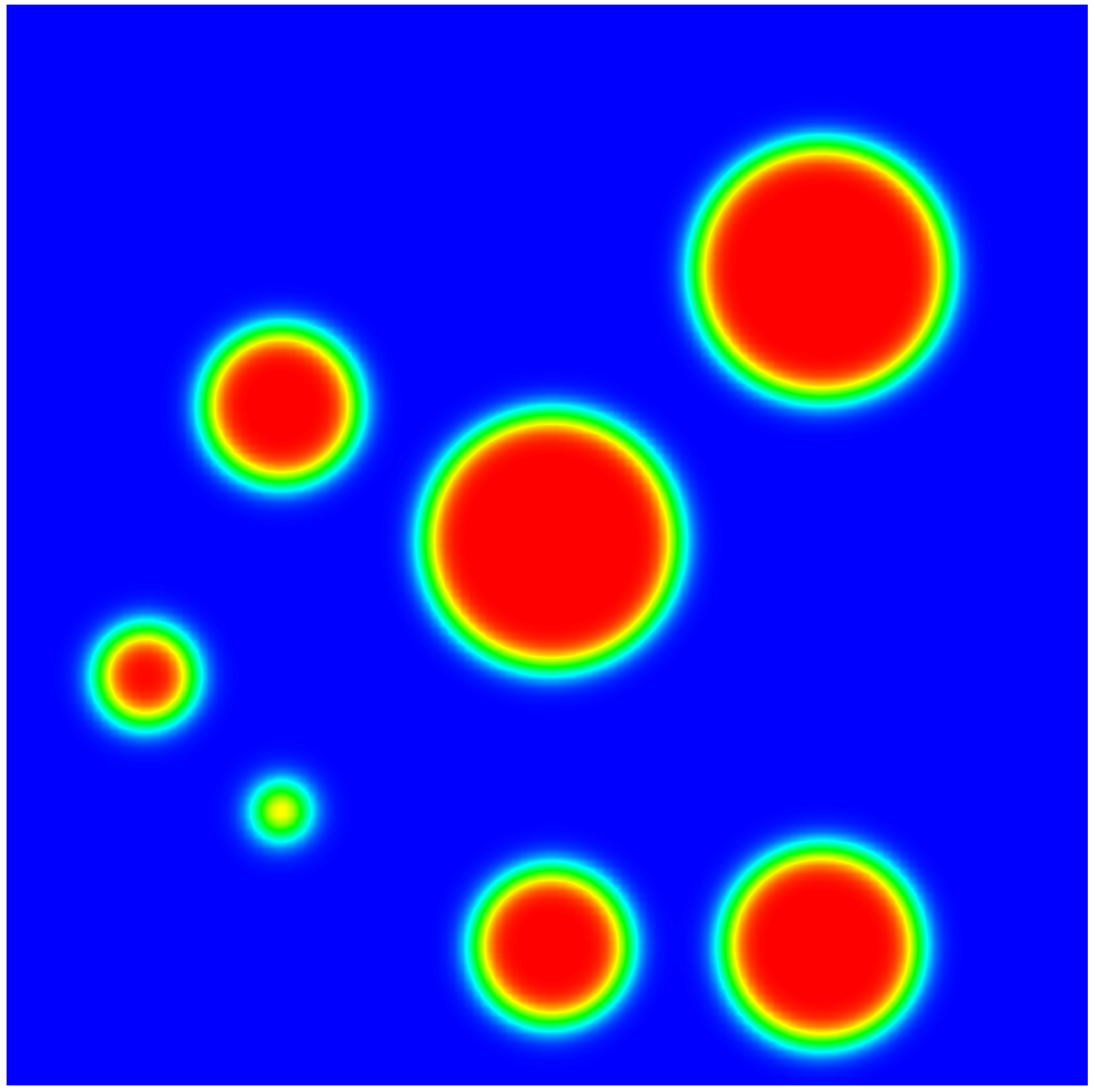
For the AC equation and the CH equation, we consider a square domain Ω=[0,1]2\Omega=[0,1]^{2} with seven disks in the 2D domain as an initial condition, similar with the problem in [1]. It is known that the disks will shrink and eventually disappear for the dynamics driven by the AC equation since the AC equation doesn’t preserve the total volume. Meanwhile, the Ostwald ripening effect will occur for the CH equation dynamics since the CH equation maintains the total volume while minimizing the interfaces. Numerical results for the two dynamics are summarized in Figure 4.1(a) and 4.1(b), respectively, where we observe the expected dynamics.

Refer to caption
Refer to caption
Refer to caption
Refer to caption
(a) dynamics driven by the AC equation with ϕ\phi at t=0,10,50,60t=0,10,50,60
Refer to caption
Refer to caption
Refer to caption
Refer to caption
(b) dynamics driven by the CH equation with ϕ\phi at t=0,10,50,100t=0,10,50,100
Figure 4.1: Evolution dynamics driven by the Allen-Cahn equation and Cahn-Hilliard equation respectively. (a) the profiles of ϕ\phi at various time slots driven by the AC equation; (b) the profiles of ϕ\phi at various time slots driven by the CH equation.

One particular focus of this letter is how the relaxed-EQ method performs compared with the baseline EQ method. We solve the problem in Figure 4.1 using both the EQ and relaxed-EQ methods with 1282128^{2} meshes and a large time step, namely, δt=0.75\delta t=0.75 for the AC equation, and δt=0.005\delta t=0.005 for the CH equation. The numerical energies using both approaches are summarized in Figure 4.2(a) and 4.2(b) respectively for the AC and CH equations. Notice both algorithms perform well when the time step is small enough. When the time step is large, the relaxed-EQ method outperforms the baseline EQ method.

Refer to caption
(a) Energy with the AC equation
Refer to caption
(b) Energy with the CH equation
Refer to caption
(c) Energy with the MBE equation
Figure 4.2: Numerical energy comparisons between the EQ method and the relaxed-EQ method. In this figure, we test the AC equation, the CH equation and the MBE equation with both numerical methods using the same time step. This figure indicates that the relaxed-EQ method provides more accurate results for all cases than the baseline EQ method with a same time step.

Furthermore, we also use both methods to solve the MBE equation. We use classical benchmark problems from [8, 5], with the same initial conditions and parameters. Due to space limitations, the numerical results are not shown. Instead, the energy evolutions using both numerical methods with a time step δt=0.001\delta t=0.001 are summarized in Figure 4.2(c). We observe that the relaxed-EQ method provides more accurate results than the EQ method for solving the MBE model as well.

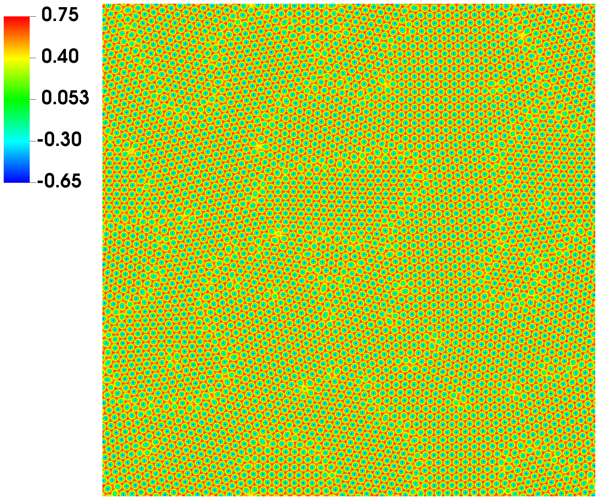
In the last example, we solve the PFC model using the relaxed-EQ scheme to further highlight its power for simulating long-time dynamics. We set up the initial conditions as Figure 4.3(a) with three pieces of crystal blocks. The numerical results of crystal growth dynamics are summarized in Figure 4.3. We observe dynamics with the appearance of micro-structure and dislocations, similarly as reported in the literature.

Refer to caption
Refer to caption
Refer to caption
(a) the profile of ϕ\phi at t=0,50,75t=0,50,75
Refer to caption
Refer to caption
Refer to caption
(b) the profile of ϕ\phi at t=100,150,1800t=100,150,1800
Figure 4.3: Microstructure evolution dynamics for triangular crystal phases driven by the phase field crystal model. The profiles of ϕ\phi at various time slots are shown.

5 Conclusion

This letter reports a relaxation technique to overcome the inconsistency issue of the modified free energy and the original energy in the energy quadratization (EQ) method. Through theorems and numerical examples, it is noticeable that the relaxed-EQ method always outperforms the baseline EQ method. In particular, it overcomes the EQ method’s primary issue that the auxiliary variable deviates from its original continuous definition after discretization as numerical errors are introduced and accumulated. In the relaxed-EQ method, the numerical solution of the auxiliary variable is relaxed towards its continuous definition in each time step with negligible computational cost. Overall, this letter’s main message is that the relaxation step shall be applied to all available EQ schemes in literature with its easy-to-use and accuracy-improving nature.

Acknowledgments

Jia Zhao would like to thank Prof. Qi Wang from the University of South Carolina for inspiring discussions on the generalized Onsager principles. Jia Zhao would also like to acknowledge the support from National Science Foundation with grant NSF-DMS-1816783, and NVIDIA Corporation for the donation of a Quadro P6000 GPU for conducting some of the numerical simulations in this paper.

References

  • [1] J. M. Church, Z. Guo, P. K. Jimack, A. Madzvamuse, K. Promislow, B. Wettona nd S. Wise, and F. Yang. High accuracy benchmark problems for allen-cahn and cahn-hilliard dynamics. Communication in Computational Physics, 26:947–972, 2019.
  • [2] Y. Gong and J. Zhao. Energy-stable Runge-Kutta schemes for gradient flow models using the energy quadratization approach. Applied Mathematics Letters, 94:224–231, 2019.
  • [3] F. Guillén-González and G. Tierra. On linear schemes for a Cahn-Hilliard diffuse interface model. Journal of Computational Physics, 234:140–171, 2013.
  • [4] D. Han and X. Wang. A second order in time uniquely solvable unconditionally stable numerical schemes for Cahn-Hilliard-Navier-Stokes equation. Journal of Computational Physics, 290(1):139–156, 2015.
  • [5] B. Li and J. G. Liu. Thin film epitaxy with or without slope selection. European Journal of Applied Mathematics, 14:713–743, 2003.
  • [6] Z. Qiao, Z. Zhang, and Tao Tang. An adaptive time-stepping strategy for the molecular beam epitaxy models. SIAM Journal on Scientific Computing, 33(3):1395–1414, 2011.
  • [7] J. Shen, J. Xu, and J. Yang. The scalar auxiliary variable (sav) approach for gradient flows. Journal of Computational Physics, 353:407–416, 2018.
  • [8] C. Wang, X. Wang, and S. Wise. Unconditionally stable schemes for equations of thin film epitaxy. Discrete and Continuous Dynamic Systems, 28(1):405–423, 2010.
  • [9] X. Yang, J. Zhao, and Q. Wang. Numerical approximations for the molecular beam epitaxial growth model based on the invariant energy quadratization method. Journal of Computational Physics, 333:102–127, 2017.
  • [10] J. Zhao, X. Yang, Y. Gong, X. Zhao, X. Yang, J. Li, and Q. Wang. A general strategy for numerical approximations of non-equilibrium models–part i thermodynamical systems. International Journal of Numerical Analysis and Modeling, 15(6):884–918, 2018.