A revisit of PSR J19093744 with 15-year high-precision timing
Abstract
We report on a high-precision timing analysis and an astrophysical study of the binary millisecond pulsar, PSR J19093744, motivated by the accumulation of data with well improved quality over the past decade. Using 15 years of observations with the Nançay Radio Telescope, we achieve a timing precision of approximately 100 ns. We verify our timing results by using both broad-band and sub-band template matching methods to create the pulse time-of-arrivals. Compared with previous studies, we improve the measurement precision of secular changes in orbital period and projected semi-major axis. We show that these variations are both dominated by the relative motion between the pulsar system and the solar system barycenter. Additionally, we identified four possible solutions to the ascending node of the pulsar orbit, and measured a precise kinetic distance of the system. Using our timing measurements and published optical observations, we investigate the binary history of this system using the stellar evolution code MESA, and discuss solutions based on detailed WD cooling at the edge of the WD age dichotomy paradigm. We determine the 3-D velocity of the system and show that it has been undergoing a highly eccentric orbit around the centre of our Galaxy. Furthermore, we set up a constraint over dipolar gravitational radiation with the system, which is complementary to previous studies given the mass of the pulsar. We also obtain a new limit on the parameterised post-Newtonian parameter, at 95% confidence level, which is fractionally better than previous best published value and achieved with a more concrete method.
keywords:
methods: data analysis — stars:pulsars: individual (PSR J19093744) — binaries: general — gravitation1 Introduction
Millisecond pulsars (MSPs) are neutron stars (NSs) that were spun up by accretion in a binary system to have a rotational period of ms (Alpar et al., 1982). They are well noted for their highly regular rotational behaviour that competes the best atomic clock on Earth over a timescale of decades (Matsakis et al., 1997; Verbiest et al., 2009). PSR J19093744, a MSP with rotational period of approximately 2.95 ms, was first discovered in the Swinburne High Latitude Pulsar Survey using the Parkes 64-m Radio Telescope (Jacoby et al., 2003). Follow-up timing campaigns have achieved a timing precision at the level of a few hundreds nano-seconds (e.g., Desvignes et al., 2016; Reardon et al., 2016; Arzoumanian et al., 2018a; Kerr et al., 2020; Alam et al., 2020a) on a timescale of over ten years, making it one of the most precisely timed pulsars. The timing datasets of PSR J19093744 have been utilized for various astrophysical experiments, including placing stringent constraint on nano-Hertz gravitational wave background (Shannon et al., 2013; Lentati et al., 2015; Arzoumanian et al., 2018b), measuring the mass of main solar system bodies (Champion et al., 2010; Caballero et al., 2018) and establishing the first pulsar time standard (Hobbs et al., 2020).
However, apart from the discovery (Jacoby et al., 2003), there has not been much work reported that focuses on the astrophysical study of the PSR J19093744 system. The significantly extended timing baseline and the largely improved data quality attributed to a state-of-the-art data recording system in the recent years, strongly motivates a revisit of this pulsar’s properties using up-to-date measurements from but not restricted to the radio timing experiment. PSR J19093744 is in a binary system with a helium-core white dwarf (He WD) companion with an orbital period of . Radio timing analysis has yielded high-precision measurement of its orbital parameters, including a few post-Keplerian parameters from which the masses of the two bodies have been determined precisely (e.g., Desvignes et al., 2016). In parallel, spectroscopy and photometry observations of the WD companion in the optical band have been used to infer its temperature, gravity, radius and radial velocity of the system (Antoniadis, 2013). The age of PSR J19093744 is of interest for resolving its formation, evolutionary and kinematic history. While characteristic (spin-down) ages of recycled pulsars are very poor true age estimators (e.g. Tauris, 2012; Tauris et al., 2012), the cooling history of their WD companions can be used to determine the age of the systems (e.g. Kulkarni et al., 1991; van Kerkwijk et al., 2005). However, this is a non-trivial exercise given that a cooling age dichotomy exists for extremely low-mass WDs (ELM WDs) depending on their hydrogen envelope thickness and the associated possibility of undergoing hydrogen shell flashes (e.g. Alberts et al., 1996; Althaus et al., 2001; Istrate et al., 2014, 2016). WD masses can also be obtained independently from radio timing data, by using optical measurements in combination with WD cooling models and the mass function of a given binary pulsar (as an example, determining the WD mass from this method also enabled a mass determination of the heavy pulsar PSR J0348+0432 by Antoniadis et al., 2013).
The same as many other NS—WD systems, PSR J19093744 is useful for a few types of gravity experiments to constrain alternative theories (Wex, 2014). The asymmetry in the gravitational binding energy of two components, one being a strongly self-gravitating NS while the other being a weakly self-gravitating WD, allows for gravitational dipolar radiative tests in a class of scalar-tensor theories which feature nonperturbative strong-field effects (Damour & Esposito-Farese, 1993, 1996; Freire et al., 2012; Shao et al., 2017). The test depends on the underlying equation of state of NS matters (Shibata et al., 2014) and, given the mass of PSR J19093744, the measurement of orbital decay could possibly place a better constraint over some equation of states. In addition, the extremely well-measured orbital eccentricity makes PSR J19093744 a superb laboratory for testing preferred-frame effects (Damour & Esposito-Farèse, 1992b; Shao & Wex, 2012; Shao et al., 2013; Shao, 2014; Will, 2014). The existence of a preferred frame in the Universe would introduce characteristic evolution in the projected semi-major axis and the orbital eccentricity vector. The absence of abnormal behaviours in them places tight constraints on two (strong-field counterparts of) parameterized post-Newtonian parameters (Will, 2018). The aforementioned tests require high precision timing of the pulsar, preferably measurements of a selection of post-Keplarian parameters and the masses of the system. PSR J19093744, as one of the most precisely timed pulsar, has already fulfilled these criteria, and provided improvements in the gravity tests.
The rest of the paper is organized as follows. In Section 2 we describe details of the observations and the post-processing of the data. Section 3 presents the results of the timing analysis, and their application to studying the binary evolution, tracking the galactic motion of the system, and testing alternative theories of gravity. Conclusions are provided in Section 4.
2 Observation
Regular timing observations of PSR J19093744 have been conducted with the Nançay Radio Telescope (NRT) since late-2004. These observations were carried out using the L-band and S-band receivers of the telescope, which have a frequency coverage of 1.1–1.8 GHz and 1.7–3.5 GHz, respectively.
Starting from late-2004, the legacy Berkeley-Orléans-Nançay (BON) backend (Cognard & Theureau, 2006), a member of the ASP/GASP coherent dedispersion backend family (Demorest, 2007), was used to record the pulsar timing data for nearly ten years, until March 2014. The bulk of the observations with the L-band receiver was conducted initially at a central frequency of 1.4 GHz and later at 1.6 GHz after August 2011, while observations with the S-band receiver were mostly performed at a central frequency of 2.0 GHz. The original bandwidth of these observations of 64 MHz was increased to 128 MHz in July 2008. Additional details about the BON dataset used in this paper are given in Desvignes et al. (2016) which presented the first Data Release from the European Pulsar Timing Array.
The Nançay Ultimate Pulsar Processing Instrument (NUPPI) is a baseband recording system using a Reconfigurable Open Architecture Computing Hardware (ROACH) FPGA board developed by the CASPER group111http://casper.berkeley.edu/ and Graphics Processing Units (GPUs). It has become the primary pulsar timing backend in operation at Nançay since August 2011 (Cognard et al., 2013). The NUPPI dataset included in this paper spans from September 2011 to July 2019. Observations with the NUPPI backend have an integration time ranging from less than 20 to over 80 min, and a bandwidth of 512 MHz which is channelised into 128 frequency channels and coherently dedispersed in each. Most of the observations with the L-band receiver were carried out at a central frequency of 1484 MHz, while those with the S-band receiver are generally centred at 2539 MHz222The central frequency of some S-band observations was set to lower frequencies of 1854 and 2154 MHz, in periods of time when the L-band receiver of Nançay was unavailable.. The data were polarisation-calibrated with the SingleAxis333http://psrchive.sourceforge.net/manuals/pac/ method of PSRCHIVE using observations of a reference noise diode conducted prior to each observation of PSR J19093744, to correct for differential phase and amplitude between the two polarisations. Then the data were phase-folded with the pulsar ephemeris from Desvignes et al. (2016) and visually checked to clean for radio frequency interference (RFI). In the case of L-band observations, the top and bottom 16 MHz of bandwidth were removed due to the presence of persistent RFI and out-of-band signal reflection in the receiver. We extracted (broad-band) Times-of-Arrivals (TOAs) from the NUPPI data444The TOAs were measured without fitting for the DM simultaneously, so that the DM modelling is left for the noise analysis stage. using the Channelised Discrete Fourier Transform (CDFT) algorithm developed in Liu et al. (2014)555The CDFT approach is integrated into a local branch of PSRCHIVE available at: https://github.com/xuanyuanstar/psrchive_CDFT.. In order to form the template profile, we integrated the top three brightest epochs, formed average profiles for each 32-MHz of bandwidth at L-band and 128-MHz of bandwidth at S-band, respectively, and removed the radiometer noise using a wavelet smoothing method. The template-matching procedure was then carried out toward data with the same frequency resolution. For the L-band data, we also divided the entire band into four 128-MHz sub-bands, formed frequency-averaged profiles and calculated the corresponding TOAs using the canonical approach detailed in Taylor (1992). These data were later used for comparison purposes as discussed in the next section. In the end, we excluded observations corrupted by calibration issues, intense RFI activity, incidental backend fault, or containing no visible pulsar signal due to interstellar scintillation. Most of the post-processing of the NUPPI data was conducted with the PSRCHIVE software package (Hotan et al., 2004). In total, the NUPPI dataset includes 405 L-band and 181 S-band observations.
3 Results
3.1 Timing analysis
3.1.1 Dataset and noise properties

We combined the BON data presented in Desvignes et al. (2016) with the NUPPI data collected in the past eight years as described above, which delivered a new dataset with an overall timing baseline of nearly fifteen years. Whenever both BON and NUPPI data were available from the same observation, we kept only the NUPPI data. In total, the dataset contains 846 TOAs, 615 at L-band and 231 at S-band. This gave us an averaged observing cadence of more than one per week. We noted that in an earlier analysis using the NUPPI data of PSR J19093744 (Liu et al., 2014), the post-processing of the data was affected by an issue in the psrchive software package666This was induced by a lack of precision in polyco epoch stored in the header of PSRFITS files. The issue was fixed by an update of psrchive in late 2014.. Reprocessing the same dataset (which contains 30 epochs from MJD 56545 to 56592) now delivers timing residuals with a weighted rms of approximately 60 ns, more than a factor of 4 better than the previous value.
We used the temponest software package to perform timing analysis to our dataset. temponest is built based on tempo2 (Hobbs et al., 2006) and multinest (Feroz et al., 2009) software packages, to explore the parameter space of a non-linear pulsar timing model with Bayesian inference (Lentati et al., 2014). The fitted parameters included in the timing model are described in Table 1 (noted as “measured parameter”). To describe the orbital motion of the pulsar in the binary system, we used the “ELL1” timing model (Lange et al., 2001) as the orbit is known to have a very small eccentricity. Additionally, we included a set of parameters to characterize the noise in the dataset. The white noise parameters are the error factor ‘EFAC’ () and an additional error added in quadrature ‘EQUAD’ () which relate to the measurement uncertainty () of a TOA as:
| (1) |
For each observing system a pair of such parameters was included to capture its white-noise properties to yield a proper weight in the data combination. To describe the long-term red process in the dataset, we included two models to account for the chromatic component caused by dispersion measure (DM) variation and the monochromatic part of the signal, respectively. In both models, the signal is assumed to be a stationary, stochastic process with a power-law spectrum in the form of
| (2) |
where , , are the power spectral density as a function of frequency , the spectral amplitude, the spectral index and the reference frequency (set to 1 yr-1), respectively. The constant is equal to for the chromatic term and is for the monochromatic term. The spectrum had a low-frequency cutoff equal to the inverse of the data span (approximately 14.6 yr), and was sampled with integer multiples of the lowest frequency up to one over fourteen days. To align the data from different systems, we included an arbitrary time offset (known as JUMP) between the reference system and each of the rest systems. Both the timing and noise parameters were simultaneously fitted for during the temponest analysis, while the JUMPs were analytically marginalised. All model parameters were sampled with uniform priors, except for EQUAD and amplitudes of the red processes for which a log-uniform prior was used.
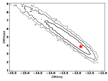
In Fig. 1 we present the timing residuals of the dataset obtained from the analysis with temponest, both before and after the subtraction of the red processes in the data. A long-term evolution of the residuals is prominent across the entire time span of the dataset, leading to an weighted rms of over 500 ns. We note that a similar feature in the PSR J19093744 timing residuals was also seen in the recent analysis presented by Arzoumanian et al. (2018a). Subtraction of the measured red noise models successfully whitened the residuals, leading to a weighted residual rms of 103 ns over a timescale of nearly fifteen years. The L-band data from NUPPI itself has a weighted residual rms of 86 ns. The posterior distribution of the red-noise parameters are presented in Fig. 2, where the logarithmic amplitude and spectral index of the achromatic red noise were measured to be and , highly consistent with published values by Caballero et al. (2016) and Arzoumanian et al. (2018a).
Timing precision of the brightest MSPs could be limited by the intrinsic variability in the pulsar signal itself which is known as “jitter noise” (e.g., Cordes & Downs, 1985; Liu et al., 2011). To estimate such contribution in our data, we selected three epoch observations when the pulsar signal was the strongest due to interstellar scintillation, and measured the jitter noise following the approach described in Liu et al. (2012). For L-band, this gave us ns, where is the amount of jitter noise with 30-min integration time. This result is well in agreement with previously published values (Shannon et al., 2014b; Lam et al., 2016, 2019). We did not measure any significant jitter noise in our S-band observation, but obtained a 95% upper limit of 78 ns for at 2.5 GHz. The limit is in line with the prediction in Lam et al. (2019) that jitter noise of PSR J19093744 should be around 10 ns at this frequency. To explore the impact of jitter noise on our noise modelling, we incorporated our measurement into the L-band data, i.e., quadratically adding the corresponding jitter noise to the TOA errors before performing the timing analysis with temponest. By doing so, the white noise description here becomes , where is calculated based on the integration time () of the observation as . In principle, the inclusion of jitter noise in the noise model would be fully covered by EQUAD if the integration times of the observations were identical (i.e., it is then a constant addition to all TOA errors just as EQUAD). This, however, is not the case here because the integration times of our observations range from 20 to 80 mins, and thus the jitter noise corresponding to each TOA can differ by up to a factor of two. Using this modified L-band dataset instead in the timing analysis gave a very minimal (well below 10%) change in EQUAD values of the L-band systems, while the EFAC values remained around unity. This is expected as the jitter noise with a typical 30-min integration time is well below the timing residual rms of the L-band data. In fact, jitter noise is dominant over the radiometer noise only in less than 1% of our observations.
To further verify our results, we carried out a separate investigation of the noise properties using the Enterprise software package which is also widely used in pulsar timing array data analysis (Ellis et al., 2019). We built the noise model consisting of the timing model, white noise and both the chromatic and achromatic red noise components. Those are the same components used in temponest, while the implementation and application are somewhat different. In detail, we performed a fully Bayesian analysis using a parallel tempering Markov Chain Monte Carlo sampler PTMCMC (Ellis & van Haasteren, 2017), adopting the same priors as in the temponest analysis but marginalising over the timing parameter errors (van Haasteren & Levin, 2012). The white noise is characterised by ‘EFAC’ and ‘EQUAD’, with the same description as in temponest (cf. Eq. 1). Both red-noise components were modelled as a stationary Gaussian process with a power-law power spectral density parameterised by an amplitude (at frequency ) and a spectral index, the same as in Eq. 2 except for that here the constant is equal to for both chromatic and monochromatic terms. The inferred posteriors, as shown in Fig. 2, are largely consistent with the results from temponest, with somewhat more pronounced tail in the distribution for the achromatic red noise distribution. This difference might be attributed to the use of different samplers (MULTINEST vs PTMCMC) in the multidimensional parameter space.
In addition, we noted that the irregularly distributed and unevenly numbered observations between L-band and S-band in the dataset may have an impact on the measurement of DM variation, in particular on separating its contribution to the overall red process from the achromatic component. To examine this potential issue and its potential impact on our timing results, we carried out the same timing analysis to a different version of the dataset where the sub-band TOAs were used for L-band observations with NUPPI. This offers more regular multi-frequency coverage and as shown in Fig. 2, thus provides better constraints on DM model parameters. The achromatic red noise parameters becomes less constrained, probably due to the drop of the best-estimated value of the amplitude. The spectral index is shifted to a higher value as expected since the effect from an “imperfect” DM modelling exhibits as a relatively shallow noise source. On the other hand, applying the noise model measurements obtained with the sub-band TOAs to subtract the red process in the original dataset resulted in very little difference in the residuals and the overall weighted rms. This suggests that our noise modelling with the broad-band TOAs should still be able to effectively extract the red processes in the data.


It is worth noting that the experimental analysis on incorporating jitter noise measurement in the TOAs and using sub-band TOAs in the dataset have both yielded highly consistent measurement in all timing parameters, compared with those from using the broad-band TOAs. This is demonstrated in Fig. 3, where the differences in measured timing parameters are shown to be all consistent with zero within 1- confidence interval. We note that in Alam et al. (2020a) and Alam et al. (2020b) the analysis using broad-band and sub-band TOAs has also led to highly consistent timing results. Thus, for the analysis in the rest of the paper we will simply quote the timing results obtained from the broad-band dataset. A more detailed noise analysis using different forms of datasets will be presented in an upcoming paper (Chalumeau et al. in prep.).

3.1.2 Astrophysical measurements
The results of the timing parameters from the analysis are summarised in Table 1, where the uncertainties of the measurements are 1- Bayesian credible interval obtained from one-dimensional marginalised posterior distribution. The posterior distributions of a subset of the timing and noise parameters from the temponest analysis can be found in Fig. 4. In Table 2 we compared a subset of timing parameters from our analysis with a few recent publications. It can be seen that all of our measurements have a broad consistency with previous analysis, and that our work has led to a clear improvement in measurement precision of and . We note that Alam et al. (2020a) reported a covariance between and the red-noise terms. This, however, is not obvious from the posteriors shown in Fig. 4, possibly because the longer timing baseline here helps to mitigate the degeneracy between and the red-noise parameters. Using the measurements of the Shapiro delay parameters, and , the mass of the pulsar and the WD are derived to be and , respectively, as demonstrated in Fig. 5. These new values resolves the slight inconsistency reported in Desvignes et al. (2016) from other works. Fig. 5 also shows the independent constraint on the mass ratio () reported in Antoniadis (2013) based on optical observations of the WD, which is consistent with the values determined from Shapiro delay, albeit with a larger uncertainty.
The orbital eccentricity can be calculated as , which still makes PSR J19093744 the most circular system in all binary pulsars known by far (Manchester et al., 2005). Using the mass measurements, the relativistic periastron advance of the system is calculated to be 0.14 deg/yr (Lorimer & Kramer, 2005). Accordingly, the eccentricity vector has rotated by only 2 deg within the fifteen years of our timing baseline, which, if unmodelled, would cause an apparent variation in the , components of the eccentricity vector by less than . This is well below their measurement precision shown in Table 1. Thus, the periastron advance is still not measurable with our dataset.


| Parameter | Value |
|---|---|
| MJD range | 5336858693 |
| Number of TOAs | 846 |
| Timing residual rms (s) | 0.103 |
| Reference epoch (MJD) | 55000 |
| Measured parameter | |
| Right ascension, (J2000) | 19:09:47.4335812(6) |
| Declination, (J2000) | 37:44:14.51566(2) |
| Proper motion in , (mas yr-1) | 9.512(1) |
| Proper motion in , (mas yr-1) | 35.782(5) |
| Parallax, (mas) | 0.861(13) |
| Spin frequency, (Hz) | 339.315687218483(1) |
| Spin frequency derivative, | |
| DM (cm-3 pc) | 10.3928(3) |
| DM1 (cm-3 pc yr-1) | 0.00035(5) |
| DM2 (cm-3 pc yr-2) | |
| Orbital period, (d) | 1.533449474305(5) |
| Epoch of ascending node (MJD), | 53113.950742009(5) |
| Projected semi-major axis, (s) | 1.89799111(3) |
| component of the eccentricity, | |
| component of the eccentricity, | |
| Orbital period derivative, | |
| Derivative of , | |
| Shape of Shapiro delay, | 0.998005(65) |
| Range of Shapiro delay, (s) | 1.029(5) |
| Derived parameter (assuming GR) | |
| Galactic longitude, (deg) | 359.7 |
| Galactic latitude, (deg) | 19.6 |
| Longitude of periastron, (deg) | 156(5) |
| Orbital eccentricity, | |
| Pulsar mass, () | 1.492(14) |
| Companion mass, () | 0.209(1) |
| Parallax distance, (kpc) | 1.16(2) |
| kinematic distance, (kpc) | 1.158(3) |
| Spin period, (ms) | 2.94710806976663(1) |
| Spin period derivative, () | 14.02521(6) |
| () | 0.0587(2) |
| () | 11.36(3) |
| () | 2.60(3) |
| Characteristic age, (Gyr) | 18.0 |
| Surface magnetic field, (G) |
| (mas) | () | |||||
|---|---|---|---|---|---|---|
| Desvignes et al. (2016) | 0.87(2) | 0.99771(13) | 0.213(2) | |||
| Reardon et al. (2016) | 0.81(3) | - | 0.99811(16) | 0.2067(19) | ||
| Arzoumanian et al. (2018a) | 0.92(3) | 0.99808(9) | 0.208(2) | |||
| Perera et al. (2019) | 0.88(1) | 0.99807(6) | 0.209(1) | |||
| Alam et al. (2020a) | 0.88(2) | 0.99794(7) | 0.210(2) | |||
| This work | 0.861(13) | 0.998005(65) | 0.209(1) |
The observed secular variation of orbital period in binary pulsars can include contributions from multiple effects (Damour & Taylor, 1991; Lorimer & Kramer, 2005). As for the case of PSR J19093744 where the pulsar has negligible tidal interaction with the WD companion, the most relevant effects can be summarised below:
| (3) |
The first term, , denotes the contribution from the transverse relative motion of the system to the solar system barycentre (SSB) which is known as the Shklovskii effect. Using the measured proper motion of the pulsar (, ) and its distance () derived from timing parallax, this term is estimated to be
| (4) |
where is the speed of light. The second term, , is caused by the differential acceleration from the Galactic potential. As shown in Damour & Taylor (1991), this effect can be calculated based on astrometric measurements and a Galactic potential model. Using our timing results and the model provided in McMillan (2017), we have777The error in this calculation only reflects the error in the parallax. Accounting for a realistic error in the Galactic potential, one expects an error roughly an order of magnitude larger, which however, is still about an order of magnitude smaller than the error in .
| (5) |
The third term, , represents the contribution from gravitational wave damping in GR, and following Peters (1964), is found to be888Whenever being in combination with , masses are understood in solar units.
| (6) |
where , and is the solar mass parameter as defined by the IAU (Mamajek et al., 2015). The last term, , is arising from the mass loss of the system. In the case of PSR J19093744, we consider the loss of rotational energy of the pulsar to be the dominant mass-loss effect, given that there is no expectation of significant stellar wind from a cooled WD with strong surface gravity like the companion of PSR J19093744 (e.g., Unglaub, 2008). Following Damour & Taylor (1991), this can be worked out as999The uncertainty here only includes the measurement error of the parameters, except whose value is assumed. It should be noted that Eq. (7) is an approximation for slowly rotating neutron stars, whose precision nevertheless is better than 10% for PSR J19093744.
| (7) |
Here and denote the moment of inertia and the intrinsic period derivative of the pulsar, respectively. To obtain the estimate above, we used g cm2, a typical value derived using our mass measurement and different equations of state that are in agreement with all pulsar and LIGO/Virgo constraints (Lattimer & Prakash, 2001; Capano et al., 2020). We also recovered the intrinsic spin period derivative, by subtracting the contribution from the Shkloskii effect and the Galactic potential from the observed value as performed in the case of the orbital period derivative. These calculations are summarized in Table 1 which shows that the intrinsic of the pulsar is in fact more than a factor of five smaller than the observed value.
The analysis above clearly shows that the observed is dominated by the Shklovskii effect, next to which is the contribution from Galactic potential. Though the expected contribution from gravitational wave damping is well above the measurement uncertainty of the observed , it is still below the estimation error of the Shklovskii contribution which mostly comes from the measurement uncertainty in parallax distance. Thus, with the current measurement precision is not separable from and we expect to be able to do so only when the precision in distance measurement is improved by at least a factor of 4 to 5. This could possibly be obtained by adding more existing data, extending the timing baseline, or using timing data from more sensitivity telescope (e.g., Bailes et al., 2018). Subtracting all aforementioned contributions from gives which is consistent with zero. This allows us to calculate the kinematic distance () of the system with by directly assuming a zero excessive (Bell & Bailes, 1996), which gives kpc, a highly consistent and more precise distance estimate.
The observed secular variation of projected semi-major axis in binary pulsars can also be induced by a series of effects as listed below (Lorimer & Kramer, 2005):
| (8) |
The first term, , stands for the contribution from the Shklovskii effect, and using our timing astrometric measurements, is estimated to be:
| (9) |
The second term, , is the contribution from the differential Galactic potential, and following the same approach as for , is found to be
| (10) |
The third term, , is caused by gravitational wave damping. Following (Peters, 1964) and using our mass measurements, it is estimated to be
| (11) |
The fourth and fifth term, 101010Here is defined as in Eq. (2.6) of Damour & Taylor (1992). and , denote contribution from geodetic precession of the pulsar spin axis and the precession of the orbital plane due to spin-orbit coupling effect (classical and/or Lense-Thirring), respectively. Following Damour & Taylor (1991), is of order . The spin-orbit precession induced by the companion’s rotation has so far been measured in a small number of different binary pulsar systems (Kaspi et al., 1996; Shannon et al., 2014a; Venkatraman Krishnan et al., 2020). However, spin-orbit contributions to vanish when the spin axes of the pulsar and companion are aligned with the orbital angular momentum (e.g., Damour & Taylor, 1992; Wex, 1998), which is expected to be the case for fully recycled binary pulsars such as PSR J19093744 from the binary evolution aspect (e.g., Tauris, 2012). Additionally, the pulsar is in a relatively wide orbit with the WD companion, which will further suppress the spin-orbit coupling effects by a few orders of magnitude compared with the case of PSR J11416545 studied in (Venkatraman Krishnan et al., 2020).
Therefore, it can be concluded that the contribution from the relative motion between the pulsar and the SSB, , should be dominating in . Following the derivations presented in Arzoumanian et al. (1996) and Kopeikin (1996), this effect can be expressed as111111Note that there is a conversion between the and here and those in Kopeikin (1996): , .
| (12) |
It can be seen that one can derive the ascending node of the binary system, , once and are measured. This is shown in Fig. 6, where we plot the contribution to from the proper motion for PSR J19093744 as a function of , in conjunction with the measured . Accordingly, we have identified four possible solutions considering the ambiguity in ( equals to the shape of Shapiro delay, ): , deg when deg, and , deg when deg. We noted that Reardon et al. (2016) reported only one possible solution of such and Alam et al. (2020a) reported two. In principle, this ambiguity can be resolved if the annual-orbital parallax of the binary system is measurable, via directly fitting for the “Kopeikin” (KOM and KIN) parameters in the tempo2 software package as e.g., has been carried out in the PSR J1713+0747 system (see e.g. Desvignes et al., 2016). However, with the formula in Kopeikin (1995), we estimate the scale of the feature in the timing data induced by annual-orbital parallax to be ns, well below any of the published timing precision of PSR J19093744. This is mostly due to the fact that PSR J19093744 has a small and edge-on orbit with a distance on order of kpc. In practice, the Kopeikin parameters can also be highly correlated with some of the Keplerian parameters (e.g., the orbital period), which would further suppress the subtractable feature from the fit. Thus, our current timing precision does not allow to distinguish among the four possible solutions by modelling the annual-orbital parallax of the system. This has been verified by our attempt to switch on the fit for the Kopeikin parameters in our analysis, where all of the four solutions can be found, resulting in the same post-fit residual rms and returning the same goodness-of-fit. We however note that studying the orbital variations in the interstellar scintillation of the pulsar could potentially provide additional constraint over orbital inclination and help to resolve the ambiguity in our solutions (e.g., Lyne, 1984; Reardon et al., 2019).

3.2 Binary evolution
PSR J19093744 is an archetypical binary MSP with an orbital period of , a helium-core WD companion of mass , a (very) low eccentricity , a rapid NS spin of , a small spin period derivative of (yielding a surface magnetic dipole field of approximately ), and a NS mass of . All these characteristics imply a plain vanilla formation scenario from a progenitor system which was a low-mass X-ray binary (LMXB) with a NS accretor and a main-sequence donor of mass (Tauris & van den Heuvel, 2006; Tauris, 2011). Donor stars less massive than about (depending on metallicity) will not terminate their evolution within a Hubble time, and stars more massive than start to burn helium without their core becoming degenerate.

.
In order to study the formation and evolution of PSR J19093744, we employed new binary evolutionary models computed with the open source stellar evolution code MESA (Paxton et al., 2011; Paxton et al., 2013, 2015, 2018), version 12115, with the assumed physics similar as presented in Istrate et al. (2016) (e.g including rotational mixing and element diffusion). The new evolutionary models will be soon available publicly (Istrate et. al 2020, in prep). For the initial binary conditions, we assumed a 1.1 donor mass, 1.3 NS accretor treated as a point mass, and an accretion efficiency of ().
From a stellar evolution point of view, one expects a tight correlation between the orbital period at the end of the LMXB phase and the mass of the proto-He WD (e.g. Savonije, 1987; Joss et al., 1987; Rappaport et al., 1995; Tauris & Savonije, 1999; Lin et al., 2011; Jia & Li, 2014; Istrate et al., 2014). This results from the relatively tight correlation existing between the degenerate-core mass of a red giant star and its radius (Refsdal & Weigert, 1971). The mass-period relation depends primarily on the assumed metallicity and to some extent on other stellar parameters, such as the adopted mixing length value, and partly on the initial donor mass (Tauris & Savonije, 1999). Our models presented below assume .

Fig. 7 shows the orbital period at the end of the LMXB phase versus the mass of the He WD for Z=0.0001, Z=0.001 and solar-like metallicity of Z=0.0142. The gray area represents the fitted mass-period relation for population I and II stars from Tauris & Savonije (1999). Over-plotted are several observed values for MSP companions for which the mass121212The values are taken from https://www3.mpifr-bonn.mpg.de/staff/pfreire/NS_masses.html. of the He WD was measured from the Shapiro delay and therefore it is independent of the WD cooling models used. One should note that the observed mass-period relation can appear to be different from the theoretical mass-period relations in Fig. 7, especially at relatively small orbital periods or alternatively small WD masses. The most important contributor to this discrepancy is the shrinkage of the orbit due to gravitational wave radiation. There are also smaller effects due to the change in the orbit as well as in mass of the WD caused by the occurrence of hydrogen shell flashes, which are stronger at higher metallicities (see for example the discussion in Mata Sánchez et al., 2020). Finally, deviations can occur due to pulsar irradiation of the donor star which results in a widening of the orbit while the WD mass decreases (Kluźniak et al., 1988; Stevens et al., 1992; van Haaften et al., 2012; Chen et al., 2013).
The observed orbital period and companion mass for PSR J19093744 are marked with a black star and are in agreement with the values predicted for Z=0.001. Notably, the companion of PSR J19093744 has one of the most accurate mass measurements from the Shapiro delay. As previously mentioned, the theoretical mass-period relations can vary based on assumed value of mixing length, . For example, it would be possible that one could find a solution for a somewhat lower metallicity than Z=0.001 with smaller than 2.0 or slightly higher metallicity than Z=0.001 with larger than 2.0. The value of is relatively uncertain and possibly is degenerate with stellar mass or metallicity (e.g Tayar et al., 2017; Viani et al., 2018; Sonoi et al., 2019; Valle et al., 2019).
Fig. 8 shows the orbital period evolution for a few selected evolutionary tracks with Z=0.001 that produce a final WD mass of 0.207, 0.208, 0.209 and 0.210 , respectively. The measured companion mass of PSR J19093744 is consistent with a 0.208, 0.209 and a 0.210 solution; however, as it can be seen from Fig. 8, the measured orbital period is only consistent with the 0.208 track. Notably, at the moment of the Roche-lobe detachment, the orbital period was slightly larger, , but after of orbital decay due to gravitational wave radiation it crosses the present value of 1.53 days (see inlet in Fig. 8).
In order to obtain the final NS mass in agreement with the observed value (), we fine-tuned the accretion efficiency, to a value of , given our assumed NS birth mass of and initial donor mass of . This value is close to the upper limit of the accretion efficiency from the following reasons: a higher initial donor mass implies a smaller value of , and a smaller initial donor mass (which would imply a larger value for ) is unlikely as the evolution of the system to the current observed values will take longer than the Hubble time.

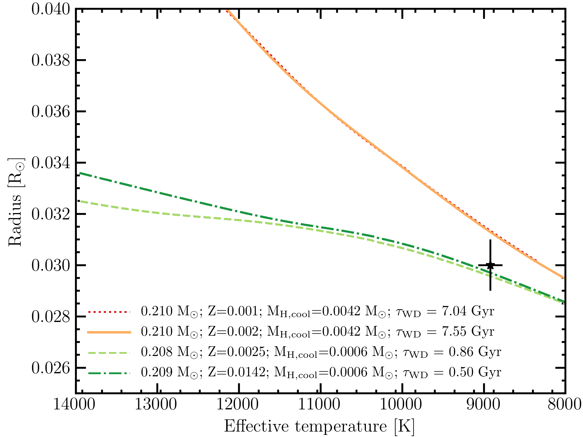
It has been demonstrated that characteristic ages, are often very poor true age estimators for recycled pulsars (Tauris, 2012; Tauris et al., 2012). Therefore, we use the cooling age of the WD, (defined as the time elapsed since the end of the LMXB phase until the WD reaches the observed effective temperature) to estimate the age of the PSR J19093744 system. The WD companion has a measured radius of 0.0300.001 R⊙(Antoniadis, 2013) and an effective temperature of 8920150 K (Kilic et al., 2018). Fig. 9 shows the evolution of the radius versus effective temperature (cooling evolution) for the selected evolutionary models presented above. None of the cooling tracks in Fig. 9 are consistent at the 1- level with the observed value of the WD radius. These cooling tracks are all characterized by a thick hydrogen envelope of with an associated WD age of the order of 7 Gyr. We therefore search for another solution to see if we can better match the derived WD radius.
The most important parameter that determines the cooling history of a WD, for a given mass, is the mass of its envelope. Helium-core WDs can be divided into thin or thick hydrogen envelopes depending on whether or not they experience diffusion-induced hydrogen shell flashes (e.g Althaus et al., 2001; Istrate et al., 2016) with a large impact on their cooling ages (the cooling dichotomy, e.g. Alberts et al., 1996; van Kerkwijk et al., 2005; Istrate et al., 2014). The mass threshold for a hydrogen flash occurrence depends strongly on the assumed metallicity (Istrate et al., 2016). This is also demonstrated in Fig. 10, where we show our computed cooling tracks for a helium-core WD of resulting from initial donors with a metallicity of Z=0.001, Z=0.002, Z=0.0025 and Z=0.0142, respectively. The mass threshold for flashes to occur at the metallicity suggested by the binary evolution, Z=0.001, is . This threshold drops to for Z=0.002. As a consequence, the upper two tracks with Z=0.001 and Z=0.002 have thick envelopes ( , and no flashes) and the bottom tracks have thin hydrogen envelopes ( , and undergo flashes). The observed properties of the PSR J19093744 companion are consistent at the 1- level only with thin hydrogen envelope models with a corresponding age of . However, at the 2- level, both thick and thin hydrogen envelope solutions are possible, with a resulting large spread in the cooling age from 7 Gyr to 0.5 Gyr, respectively. Given the current uncertainties of the radius, one cannot firmly derive the cooling age of the WD and therefore the age of the pulsar.
We stress here that the binary evolutionary models leading to a He WD orbiting a MSP use various parameters that are not well constrained yet. At the level of precision that we investigated in this work, parameters such as , overshooting, initial donor mass, efficiencies of various mixing processes, just to name a few, play an important role in determining the precise mass-period relation at a given metallicity. Varying these parameters, one could obtain a thin hydrogen envelope solution self-consistently from the binary evolution in the same manner as the solution presented for the thick envelopes. Alternatively, the mass threshold for flash occurrence as well as the amount of hydrogen remaining after the hydrogen-shell flash episodes might also depend on other physical parameters besides the well-known dependence on element diffusion (e.g Althaus et al., 2001; Istrate et al., 2014, 2016)). Once a more precise and reliable radius measurement can be obtained, the PSR J19093744 system will serve as a powerful benchmark for investigating the influence and calibrating parameters that otherwise are thought to have only second-order effects both for the binary evolution and cooling of helium-core WDs.
To summarise, we have obtained a binary solution in agreement with the observed orbital period, WD mass and NS mass for Z=0.001, with an upper limit for the accretion efficiency . However, this solution is not self-consistent with the cooling properties of the PSR J19093744 WD companion. The radius, effective temperature and mass of the WD can best be explained by models with a thin hydrogen envelope (most likely with a chemical abundance Z ) with a corresponding age of only , but at the 2- level, the cooling age varies from 7 Gyr to 0.5 Gyr. We emphasise here that the WD companion to PSR J19093744 is a perfect showcase for the cooling dichotomy of He WDs, which makes an age determination very difficult in practice. To pinpoint with certainty a cooling age, one would need a more accurate radius measurement. Currently, this is mostly limited by uncertainties in the reddening estimate, and the precision of available photometric data. Therefore, a significant improvement would require deeper imaging observations at multiple wavelengths and a more precise extinction model.
Fortunately, the effective temperature and the surface gravity of the WD companion of PSR J19093744 place it closely to the red edge of the instability strip of extremely-low mass white dwarf variable stars (ELMVs) (Córsico et al., 2012; Van Grootel et al., 2013; Kilic et al., 2018). Additional constraints on the thickness of the hydrogen envelope (and therefore cooling age) could be obtained if one would investigate the asteroseismological properties for the possible evolutionary solutions and (ideally) compare it with observed pulsation periods (Calcaferro et al., 2018). This is beyond the scope of this paper and it will be addressed in a future work.
3.3 3D velocity and Galactic motion
PSR J19093744 is one of the few pulsars where we have full information on the 3D spatial velocity with respect to the SSB. The proper motions in right ascension and declination are known with high precision from timing observations (see Tab. 1). The same is the case for the distance to the PSR J19093744 system. In particular, the kinematic distance has an uncertainty of less than 0.3%. Combining this information gives a transverse velocity of . Finally, from high-resolution spectroscopy Antoniadis (2013) was able to infer a systemic radial velocity of with respect to the SSB. The corresponding total velocity with respect to the SSB is found to be .
With the local (SSB frame) position and 3D velocity of PSR J19093744 at hand, we can now reconstruct the Galactic motion of the PSR J19093744 system. For this purpose, we make use of the Galactic gravitational potential given by McMillan (2017). We introduce a Galactic frame centered at the location of the Galactic center, with the plane coinciding with the Galactic plane, and the Sun located at kpc and kpc. For the purpose of this section, we can safely ignore the small and somewhat uncertain offset of the Sun from the Galactic plane (see e.g. Yao et al., 2017). The value for the Sun corresponds to the Galactic center distance used in the McMillan (2017) model, which is in good agreement with the latest distance estimate for Sgr A∗ by the GRAVITY Collaboration (Gravity Collaboration et al., 2020). To calculate today’s velocity of the PSR J19093744 system with respect to our frame, we need the Galactic velocity vector of the SSB. For a given , the proper motion measurements for Sgr A∗ by Reid & Brunthaler (2004) can directly be converted into the - and -velocity of the SSB. For kpc we find and . Furthermore, we adopt , in agreement with McMillan (2017) as well as Reid et al. (2014). As a result, we find the following Galactic velocity for PSR J19093744
| (13) | |||||
| (14) | |||||
| (15) |
The small error in does not come as a surprise. On one hand, the error budget in the velocity is clearly dominated by the error in the observed radial velocity; on the other, PSR J19093744 is located at and (see Tab. 1), meaning that the radial velocity has practically no component in -direction. Furthermore, it is interesting to note how small is, compared to the motion of the SSB, i.e. , although PSR J19093744 is practically in our Galactic neighbourhood. From this, one can already assess that the PSR J19093744 must have a somewhat peculiar Galactic motion. The velocity with respect to its local standard of rest is therefore comparatively large, amounting to .
We have used the software package provided by McMillan (2017) to integrate the Galactic motion of the PSR J19093744 system back in time, using its current location and inverting its current velocity in Eqs. (13)–(15). The result is given in Fig. 11, where we have stopped the integration at 500 Myr, which is below the expected age of the pulsar, i.e. long after the supernovae that formed the neutron star and imparted a kick to the system (see Section 3.2). As one can see, PSR J19093744 is on a highly eccentric orbit, currently being close to its maximum distance from the Galactic center. About 30 Myr ago it had its closest approach to the Galactic center with a distance of kpc. The motion is confined to a region comparably close to the Galactic plane with kpc. We have used different models for the Galactic potential (provided with the software package of McMillan (2017)) to verify the robustness of our finding against uncertainties in the Galactic gravitational potential. The fine details of the Galactic orbit of PSR J19093744 should generally be taken with a grain of salt, since already the assumption of an axisymmetric mass distribution in our Galaxy is only a first order approximation. For instance, in the inner few kpc one has the central bar as a clearly non-axisymmetric structure (see Bland-Hawthorn & Gerhard, 2016, and references therein). Although this will modify the details of the orbit, it is not expected to change the overall picture that the Galactic orbit of PSR J19093744 is highly eccentric and takes PSR J19093744 into the inner Galactic region.

3.3.1 On the small eccentricity of PSR J19093744
The orbital eccentricity of PSR J19093744 is a record low among all known binary pulsars with a value of just . Given a potential age of from 0.5 to 7 Gyr of this binary pulsar (inferred from the WD cooling age, as discussed in Section 3.2), it is of interest to investigate whether we can use it as a probe of the stellar density in the Galactic disk. It is anticipated that orbital eccentricities might be induced by dynamical interactions with field stars, similar to the examples of resulting high eccentricities seen among some binary pulsars in dense stellar environments like globular clusters. The question is if for an assumed old system like PSR J19093744 (depending on the exact WD cooling models discussed in Section 3.2), the column density of field stars within its cross-section radius, accumulated from its motion in the disk (Section 3.3) over its lifetime of several Gyr, may reach a critical level.
Rasio & Heggie (1995) investigated resulting eccentricities of binary MSPs induced via such dynamical interactions, and they derived the following expression (their Eq. 6):
| (16) |
where , and is the age in units of Gyr, is the stellar density (all assumed to be of mass ) in units of , and being the one-dimensional velocity dispersion in units of . Given and , it yields . Assuming (based on the relative velocity between PSR J19093744 and local field stars), and as an extreme upper limit, we find that . I.e. the critical number density needed to explain the small observed eccentricity of for PSR J19093744 based on dynamical interactions is about . This value is four orders of magnitude larger that the number density of stars in the solar neighborhood, (e.g., Holmberg & Flynn, 2000).
Therefore, we conclude that it is not surprising that PSR J19093744 was able to retain its small eccentricity although potentially plowing through the Galactic disk for possibly up to several Gyr. We also note that this eccentricity is expected to be a residual value from its formation process via mass transfer from the progenitor star of the WD (Phinney, 1992).
3.4 Tests of alternative gravity theories
3.4.1 Testing for dipolar radiation
Short orbital period ( d) pulsar-WD systems have turned out to provide some of the most stringent limits on dipolar gravitational radiation, a prediction by many alternative gravity theories (Wex, 2014). With its orbital period of approximately 1.5 days, PSR J19093744 is rather slow compared to the systems like PSR J1738+0333 (Freire et al., 2012) or PSR J0348+0432 (Antoniadis et al., 2013). However, its outstanding timing precision and the corresponding precise measurement of makes it still interesting for a test of dipolar gravitational wave damping. Moreover, while for PSR J1738+0333 and PSR J0348+0432 optical measurements and the modelling of WD spectra were required to obtain the masses of pulsar and companion, for PSR J19093744 we can estimate these masses directly from the high precision timing observations due to the presence of a prominent Shapiro delay.
Here we discuss our dipolar radiation test within the framework of Bergmann-Wagoner theories. Bergmann-Wagoner theories represent the most general mono-scalar–tensor theories that are at most quadratic in the derivatives of the fields in their action (Will, 2018). Quite a number of well known mono-scalar-tensor theories belong to this class, like Jordan-Fierz-Brans-Dicke (JFBD) gravity (Jordan, 1955; Fierz, 1956; Brans & Dicke, 1961), DEF gravity (Damour & Esposito-Farese, 1993, 1996), MO gravity (Mendes & Ortiz, 2016), gravity (De Felice & Tsujikawa, 2010), and massive Brans-Dicke gravity (Alsing et al., 2012).
In Bergmann-Wagoner theories, the field equations for the (physical) “Jordan-frame metric” and the scalar field can be derived from the following action
| (17) | |||||
where denotes the fundamental (“bare”) gravitational constant, is the determinant of the metric , and the curvature scalar. The two functions and denote the coupling function and the scalar potential, respectively. Here we will assume that the influence of is negligible on the relevant scales (cf. Alsing et al., 2012). is the action of the matter fields , which couple universally to the spacetime metric .
The Newtonian gravitational constant, as measured in a Cavendish-type experiment, is given by
| (18) |
where is the cosmological background field and . A further quantity, which we will need below, is the sensitivity
| (19) |
which accounts for the dependence of the mass of the -th body (for a fixed number of baryons) on a change in its ambient scalar field (Will, 2018).
For our dipolar radiation test with PSR J19093744 we can utilize three post-Keplerian parameters. These are the range
| (20) |
and shape
| (21) |
of the Shapiro delay caused by the WD companion, and a potential (intrinsic) change of the orbital period due to scalar dipolar radiation
| (22) |
where . In Eq. (22) we have neglected the dependence on the eccentricity, since the PSR J19093744 orbit is practically circular. The sensitivity of the WD companion has been neglected as well, since generally (see e.g. Will, 2018, for details). In principle, also has additional multipole contributions, dominated by the tensorial quadrupole (Damour & Esposito-Farese, 1992a; Will, 2018). They are all well below the current measurement precision (cf. Eqs. 6) and (23)) and therefore can be ignored in the following calculations.
While due to Solar system experiments (Bertotti et al., 2003), one cannot a priori assume that and are small as well. In fact, within Damour–Esposito-Farèse gravity it has been found that can be of order unity even if . In this regime of the so-called “spontaneous scalarization” the strong-field gravity of a neutron star can lead to very large sensitivities, .
For a given theory, i.e. a given , and a given equation of state for neutron star matter, one can calculate the sensitivity , and use the three post-Keplerian parameters, i.e. Eqs. (20–22), with the two unknown masses as a consistency test (see e.g. Damour & Taylor, 1992). Here we will follow a more generic approach by leaving unspecified and only making use of the Solar system constraint on . For a given , Eqs. (20–22) can then be solved for , , and .
The numerical values for the Shapiro range in Eq. (20) and the Shapiro shape (21) can directly be taken from Table 1: and . In Eq. (22) we need the intrinsic change of the orbital period, i.e. we need to subtract Shklovskii () and Galactic () contributions from the observed orbital period derivative in Table 1 (see e.g. Lorimer & Kramer, 2005). Using the parallax distance from Table 1 and the Galactic potential of McMillan (2017) we find for the intrinsic change of the orbital period
| (23) |
It is worth mentioning that as discussed in Section 3.1.2, the observed secular change in orbital period is predominantly coming from the Shklovskii contribution. There is no measurable intrinsic orbital period change, as one can see from Eq. (23), and the Galactic correction is only and therefore smaller than the error in the Shklovskii correction. For comparison, with the masses from Table 1 one finds for the orbital period change as predicted by the GR’s quadrupole formula (see Eq. (6)), significantly smaller than the error in .
With the numbers for the three post-Keplerian parameters in hand, we can now use Eqs. (20–22) to calculate the mass parameters and and put generic (i.e. independent of the details of ) constraints on combinations of and . As it turns out, for the allowed range of the constraints on do come exclusively from Eq. (22). As a result, for all values of compatible with Solar system experiments one has
| (24) |
In a comparison with the currently best limit on dipolar radiation obtained from PSR J1738+0333 (Freire et al., 2012; Zhu et al., 2019) one has to keep in mind that (Will, 2018). Assuming Eq. (7) in Zhu et al. (2019) for the sensitivity, in order to make the limit comparable, one obtains from Eq. (24)
| (25) |
This limit is still about an order of magnitude weaker than the one from PSR J1738+0333. Nevertheless, the limit is qualitatively different as it is based on three post-Keplerian parameters, while the PSR J1738+0333 limit used optical observations and WD models to obtain the masses of pulsar and companion. As a result, the mass of PSR J19093744 is known with higher precision (better than 1%; see Tab. 1), which is important for strong field effects that depend critically on the neutron-star mass. In Fig. 12 we give a specific example to illustrate this.

3.4.2 Testing for a preferred frame for gravity
High-precision timing with binary pulsars is a also powerful tool in constraining the gravitational Lorentz invariance violation via its orbital dynamics. This type of study is typically carried out using the parameterized post-Newtonian (PPN) formalism (Will, 2014; Wex, 2014; Shao & Wex, 2016; Will, 2018). Here we investigate the application of the PSR J19093744 system to such gravity experiments.
In the PPN framework, Lorentz invariance violation is described by three PPN parameters, , , and . While and only pertain to semi-conservative dynamics, additionally introduces nonconservative effects, namely, it simultaneously introduces preferred-frame effects and violates the energy-momentum conservation laws (Will, 2014, 2018). The parameter was severely bound, down to the level of , via the long-term high-precision timing of PSR J1713+0747 (Zhu et al., 2019). Therefore, here we only consider constraints of and . Because neutron stars are strongly self-gravitating objects, in order to distinguish them from weak-field objects, in the following we use and respectively to denote the strong-field counterparts of and .
As shown in Shao & Wex (2012), for a nearly circular binary orbit, introduces a precession of the orbital angular momentum around the direction of , where is the absolute velocity of the binary with respect to a preferred frame. Usually, the frame wherein the cosmic microwave background (CMB) is isotropic is chosen. The -induced precession causes the change of the orientation of the orbit with respect to the observer, notably that the orbital inclination angle is changing. This change introduces a nonzero time derivative of the projected semi-major axis, and can be bound via the timing parameter . The contribution is given by (Shao & Wex, 2012),
| (26) |
where , is the angle between and the orbital norm , and is the angle between and the direction of ascending node. As discussed in Section 3.1, for PSR J19093744 the proper motion effect is able to fully account for the observed . Hence, there is no need to have a nonzero in order to reproduce the measured , which is in fact translated into a bound on .

We follow the method developed in Shao & Wex (2012) to obtain the upper limit on . We randomize orbital ascending node uniformly in , and give equal probabilities to the configuration and the configuration . We subtract the contribution to from the proper motion (12) and assign the remaining to the -induced precession (26). Such a treatment renders the test a probabilistic one (see Sec. 3 in Shao & Wex, 2012), thus the obtained results on should only be interpreted as upper bounds (see Fig. 13). In the test, the CMB frame is chosen to be the preferred frame, and the absolute 3-dimensional systematic velocity is obtained for the binary by combining radio timing and optical observations (Antoniadis, 2013). All uncertainties in relevant parameters are taken into account in the Monte Carlo simulations. The probability density for is given in Fig. 13, from where we have,
| (27) | ||||
| (28) |
These limits are weaker than the best existing limit from the spin precession of the Sun (Nordtvedt, 1987) and solitary pulsars (Shao et al., 2013), yet it still represents a new modest limit from a completely different system.
As for the PPN parameter , Damour & Esposito-Farèse (1992b) elegantly picturised the orbital polarization phenomenon for near-circular binary orbits. In this picture, a nonzero induces a polarization of the eccentricity vector, where is the direction to the periastron. The polarization is towards a direction in the orbital plane that is perpendicular to the absolute velocity. Consequently, the observed eccentricity vector is a vectorial superposition of a constant-length, relativistically rotating eccentricity, , and a forced eccentricity, ,
| (29) |
The forced eccentricity is given by (Damour & Esposito-Farèse, 1992b; Shao & Wex, 2012),
| (30) |
where , with the effective gravitational constant and . The in Eq. (30) is the constantly rotating rate of , which, in GR, is the well-known periastron advance rate.
The above picture was applied in Shao & Wex (2012) to PSRs J1012+5307 and J1738+0333, and the yet tightest limit on was achieved. The test used the observed eccentricity, decomposed into the Laplace parameters and (Lange et al., 2001). It requires that the -introduced time variations in and to be consistent with their observed uncertainties (Shao & Wex, 2012). The best constraint, at the 95% confidence level, comes from PSR J1738+0333 (Freire et al., 2012).
To obtain constraint on with PSR J19093744, we repeated the same timing analysis as described in Section 3.1.1, with time derivatives of and ( and ) directly included as fitted timing parameters. This allowed us to have high-precision measurements of both and and their time derivatives, and enabled us to perform a more straightforward test of by directly using the time derivative of . With a nonzero , after averaging over an orbital timescale, we have (Shao & Wex, 2012)
| (31) |
where , and is the projection of onto the orbital plane.

We set up Markov-chain Monte Carlo simulations which account for all the uncertainties. For each value of , we use the emcee package (Foreman-Mackey et al., 2013) to explore the posterior distribution of that is consistent with both and . From the posterior, we obtain the median, as well as the 1-, 2-, and 3- enclosed regions for . The result for the configuration is given in Fig. 14, while the other configuration with is merely a mirrored case of Fig. 14 (see e.g. Figs. 6 & 7 in Shao & Wex, 2012). From the figure, we see that the loosest limit is from ,
| (32) | ||||
| (33) |
The limit is slightly worse than that from PSR J1738+0333. If we assume that the limit from the spin precession of solitary pulsars (Nordtvedt, 1987; Shao et al., 2013) is applicable to PSR J19093744, we can use Eq. (12) to determine (cf. Fig. 6). The corresponding allowed values of are indicated by the gray bands in Fig. 14, from which we can obtain,
| (34) | ||||
| (35) |
The limit is fractionally better than that from PSR J1738+0333. More importantly, our limit here is obtained via a more straightforward method, directly using Eq. (31), and sophisticated statistical analysis was carried out using the Bayesian inference.
4 Conclusions
In this paper, we presented a high-precision timing analysis and an astrophysical study of the binary millisecond pulsar, PSR J19093744. We have managed to achieve a timing precision of approximately 100 ns with 15 years of data collected with the Nançay Radio Telescope. The measurements out of the timing analysis have been examined by using broad-band and sub-band TOA datasets, by incorporating jitter noise in the TOA errors and by conducting the analysis with different software (temponest and enterprise). We have improved measurement precision of secular changes in orbital period and projected semi-major axis, and showed that these measured variations are dominated by the relative motion between the pulsar system and the barycenter. Using the orbital period derivative measurement, we derived a kinematic distance of the system which is highly consistent and more precise than the parallax distance. In addition, we identified four possible solutions to the ascending node of the pulsar orbit with the secular change in the projected semi-major axis.
By combining our timing measurements and published observations of the WD companion, we investigated the binary evolution history of the PSR J19093744 system by modelling with the stellar evolution code MESA, and discussed solutions based on detailed WD cooling at the edge of the WD age dichotomy paradigm. We additionally determined the 3-D velocity of the system and depicted its highly eccentric orbit around the centre of our Galaxy. Moreover, we placed a constraint over dipolar gravitational radiation, a complement to previous studies given the precisely measured mass of the pulsar. We derived an improved limit on the (strong-field counterpart of) PPN parameter, at 95% confidence level, achieved with a more concrete method than previous analysis.
Acknowledgements
We are grateful to V. Venkatraman Krishnan for valuable discussions. We also would like to thank the anonymous referee for providing very constructive comments that have helped to improve the manuscript. KL, GD and NW are supported by the European Research Council for the ERC Synergy Grant BlackHoleCam under contract no. 610058. LS was supported by the National Natural Science Foundation of China (11975027, 11991053, 11721303), the Young Elite Scientists Sponsorship Program by the China Association for Science and Technology (2018QNRC001), and the Max Planck Partner Group Program funded by the Max Planck Society. AGI acknowledges support from the Netherlands Organisation for Scientific Research (NWO) and is thankful for very productive discussions with Gijs Nelemans, Alejandra Romero, Gabriel Lauffer and Pablo Marchant. The Nançay Radio Observatory is operated by the Paris Observatory, associated with the French Centre National de la Recherche Scientifique. We acknowledge financial support from the Action Fédératrice PhyFOG funded by Paris Observatory and from “Programme National Gravitation, Références, Astronomie, Métrologie” (PNGRAM) funded by CNRS/INSU-IN2P3-INP, CEA and CNES, France.
Data Availability
The timing data used in this article shall be shared on reasonable request to the corresponding author.
References
- Alam et al. (2020a) Alam M. F., et al., 2020a, arXiv e-prints, p. arXiv:2005.06490
- Alam et al. (2020b) Alam M. F., et al., 2020b, arXiv e-prints, p. arXiv:2005.06495
- Alberts et al. (1996) Alberts F., Savonije G. J., van den Heuvel E. P. J., Pols O. R., 1996, Nature, 380, 676
- Alpar et al. (1982) Alpar M. A., Cheng A. F., Ruderman M. A., Shaham J., 1982, Nature, 300, 728
- Alsing et al. (2012) Alsing J., Berti E., Will C. M., Zaglauer H., 2012, Phys. Rev. D, 85, 064041
- Althaus et al. (2001) Althaus L. G., Serenelli A. M., Benvenuto O. G., 2001, MNRAS, 324, 617
- Antoniadis (2013) Antoniadis J. I., 2013, PhD thesis, University of Bonn
- Antoniadis et al. (2013) Antoniadis J., et al., 2013, Science, 340, 448
- Arzoumanian et al. (1996) Arzoumanian Z., Joshi K., Rasio F., Thorsett S. E., 1996, in Johnston S., Walker M. A., Bailes M., eds, Pulsars: Problems and Progress, IAU Colloquium 160. Astronomical Society of the Pacific, San Francisco, pp 525–530
- Arzoumanian et al. (2018a) Arzoumanian Z., et al., 2018a, ApJS, 235, 37
- Arzoumanian et al. (2018b) Arzoumanian Z., et al., 2018b, ApJ, 859, 47
- Bailes et al. (2018) Bailes M., et al., 2018, arXiv e-prints, p. arXiv:1803.07424
- Bell & Bailes (1996) Bell J. F., Bailes M., 1996, ApJ, 456, L33
- Bertotti et al. (2003) Bertotti B., Iess L., Tortora P., 2003, Nature, 425, 374
- Bland-Hawthorn & Gerhard (2016) Bland-Hawthorn J., Gerhard O., 2016, ARA&A, 54, 529
- Brans & Dicke (1961) Brans C., Dicke R. H., 1961, Physical Review, 124, 925
- Caballero et al. (2016) Caballero R. N., et al., 2016, MNRAS, 457, 4421
- Caballero et al. (2018) Caballero R. N., et al., 2018, MNRAS, 481, 5501
- Calcaferro et al. (2018) Calcaferro L. M., Córsico A. H., Althaus L. r. G., Romero A. D., Kepler S. O., 2018, A&A, 620, A196
- Capano et al. (2020) Capano C. D., et al., 2020, Nature Astronomy, 4, 625
- Champion et al. (2010) Champion D. J., et al., 2010, ApJ, 720, L201
- Chen et al. (2013) Chen H.-L., Chen X., Tauris T. M., Han Z., 2013, ApJ, 775, 27
- Cognard & Theureau (2006) Cognard I., Theureau G., 2006, in IAU Joint Discussion.
- Cognard et al. (2013) Cognard I., Theureau G., Guillemot L., Liu K., Lassus A., Desvignes G., 2013, in Cambresy L., Martins F., Nuss E., Palacios A., eds, SF2A-2013: Proceedings of the Annual meeting of the French Society of Astronomy and Astrophysics. pp 327–330
- Cognard et al. (2017) Cognard I., et al., 2017, ApJ, 844, 128
- Cordes & Downs (1985) Cordes J. M., Downs G. S., 1985, ApJS, 59, 343
- Córsico et al. (2012) Córsico A. H., Romero A. D., Althaus L. G., Hermes J. J., 2012, A&A, 547, A96
- Damour & Esposito-Farese (1992a) Damour T., Esposito-Farese G., 1992a, Classical and Quantum Gravity, 9, 2093
- Damour & Esposito-Farèse (1992b) Damour T., Esposito-Farèse G., 1992b, Phys. Rev. D, 46, 4128
- Damour & Esposito-Farese (1993) Damour T., Esposito-Farese G., 1993, Phys. Rev. Lett., 70, 2220
- Damour & Esposito-Farese (1996) Damour T., Esposito-Farese G., 1996, Phys. Rev. D, 54, 1474
- Damour & Taylor (1991) Damour T., Taylor J. H., 1991, ApJ, 366, 501
- Damour & Taylor (1992) Damour T., Taylor J. H., 1992, Phys. Rev. D, 45, 1840
- De Felice & Tsujikawa (2010) De Felice A., Tsujikawa S., 2010, Living Reviews in Relativity, 13, 3
- Demorest (2007) Demorest P. B., 2007, PhD thesis, University of California, Berkeley
- Desvignes et al. (2016) Desvignes G., et al., 2016, MNRAS, 458, 3341
- Ding et al. (2020) Ding H., Deller A. T., Freire P., Kaplan D. L., Lazio T. J. W., Shannon R., Stappers B., 2020, ApJ, 896, 85
- Ellis & van Haasteren (2017) Ellis J., van Haasteren R., 2017, jellis18/PTMCMCSampler: Official Release, doi:10.5281/zenodo.1037579, https://doi.org/10.5281/zenodo.1037579
- Ellis et al. (2019) Ellis J. A., Vallisneri M., Taylor S. R., Baker P. T., 2019, ENTERPRISE: Enhanced Numerical Toolbox Enabling a Robust PulsaR Inference SuitE, http://ascl.net/1912.015
- Feroz et al. (2009) Feroz F., Hobson M. P., Bridges M., 2009, MNRAS, 398, 1601
- Fierz (1956) Fierz M., 1956, Helvetica Physica Acta, 29, 128
- Foreman-Mackey et al. (2013) Foreman-Mackey D., Hogg D. W., Lang D., Goodman J., 2013, PASP, 125, 306
- Freire et al. (2012) Freire P. C. C., et al., 2012, MNRAS, 423, 3328
- Gravity Collaboration et al. (2020) Gravity Collaboration et al., 2020, A&A, 636, L5
- Hobbs et al. (2006) Hobbs G. B., Edwards R. T., Manchester R. N., 2006, MNRAS, 369, 655
- Hobbs et al. (2020) Hobbs G., et al., 2020, MNRAS, 491, 5951
- Holmberg & Flynn (2000) Holmberg J., Flynn C., 2000, MNRAS, 313, 209
- Hotan et al. (2004) Hotan A. W., van Straten W., Manchester R. N., 2004, PASA, 21, 302
- Istrate et al. (2014) Istrate A. G., Tauris T. M., Langer N., Antoniadis J., 2014, A&A, 571, L3
- Istrate et al. (2016) Istrate A. G., Marchant P., Tauris T. M., Langer N., Stancliffe R. J., Grassitelli L., 2016, A&A, 595, A35
- Jacoby et al. (2003) Jacoby B. A., Bailes M., van Kerkwijk M. H., Ord S., Hotan A., Kulkarni S. R., Anderson S. B., 2003, ApJ, 599, L99
- Jia & Li (2014) Jia K., Li X. D., 2014, ApJ, 791, 127
- Jordan (1955) Jordan P., 1955, Schwerkraft und Weltall. Die Wissenschaft, Vieweg, https://books.google.de/books?id=VP85AQAAIAAJ
- Joss et al. (1987) Joss P. C., Rappaport S., Lewis W., 1987, ApJ, 319, 180
- Kaspi et al. (1996) Kaspi V. M., Bailes M., Manchester R. N., Stappers B. W., Bell J. F., 1996, Nature, 381, 584
- Kerr et al. (2020) Kerr M., et al., 2020, arXiv e-prints, p. arXiv:2003.09780
- Kilic et al. (2018) Kilic M., et al., 2018, MNRAS, 479, 1267
- Kluźniak et al. (1988) Kluźniak W., Ruderman M., Shaham J., Tavani M., 1988, Nature, 334, 225
- Kopeikin (1995) Kopeikin S. M., 1995, ApJ, 439, L5
- Kopeikin (1996) Kopeikin S. M., 1996, ApJL, 467, L93
- Kulkarni et al. (1991) Kulkarni S. R., Djorgovski S., Klemola A. R., 1991, ApJ, 367, 221
- Lam et al. (2016) Lam M. T., et al., 2016, ApJ, 819, 155
- Lam et al. (2019) Lam M. T., et al., 2019, ApJ, 872, 193
- Lange et al. (2001) Lange C., Camilo F., Wex N., Kramer M., Backer D., Lyne A., Doroshenko O., 2001, MNRAS, 326, 274
- Lattimer & Prakash (2001) Lattimer J. M., Prakash M., 2001, ApJ, 550, 426
- Lentati et al. (2014) Lentati L., Alexander P., Hobson M. P., Feroz F., van Haasteren R., Lee K. J., Shannon R. M., 2014, MNRAS, 437, 3004
- Lentati et al. (2015) Lentati L., et al., 2015, MNRAS, 453, 2576
- Lin et al. (2011) Lin J., Rappaport S., Podsiadlowski P., Nelson L., Paxton B., Todorov P., 2011, ApJ, 732, 70
- Liu et al. (2011) Liu K., Verbiest J. P. W., Kramer M., Stappers B. W., van Straten W., Cordes J. M., 2011, MNRAS, 417, 2916
- Liu et al. (2012) Liu K., Keane E. F., Lee K. J., Kramer M., Cordes J. M., Purver M. B., 2012, MNRAS, 420, 361
- Liu et al. (2014) Liu K., et al., 2014, MNRAS, 443, 3752
- Lorimer & Kramer (2005) Lorimer D. R., Kramer M., 2005, Handbook of Pulsar Astronomy. Cambridge University Press, Cambridge, England
- Lyne (1984) Lyne A. G., 1984, Nature, 310, 300
- Mamajek et al. (2015) Mamajek E. E., et al., 2015, IAU 2015 Resolution B3 on Recommended Nominal Conversion Constants for Selected Solar and Planetary Properties (arXiv:1510.07674)
- Manchester et al. (2005) Manchester R. N., Hobbs G. B., Teoh A., Hobbs M., 2005, AJ, 129, 1993
- Mata Sánchez et al. (2020) Mata Sánchez D., Istrate A. G., van Kerkwijk M. H., Breton R. P., Kaplan D. L., 2020, arXiv e-prints, p. arXiv:2004.02901
- Matsakis et al. (1997) Matsakis D. N., Taylor J. H., Eubanks T. M., 1997, A&A, 326, 924
- McMillan (2017) McMillan P. J., 2017, MNRAS, 465, 76
- Mendes & Ortiz (2016) Mendes R. F. P., Ortiz N., 2016, Phys. Rev. D, 93, 124035
- Nordtvedt (1987) Nordtvedt K., 1987, ApJ, 320, 871
- Paxton et al. (2011) Paxton B., Bildsten L., Dotter A., Herwig F., Lesaffre P., Timmes F., 2011, ApJS, 192, 3
- Paxton et al. (2013) Paxton B., et al., 2013, ApJS, 208, 4
- Paxton et al. (2015) Paxton B., et al., 2015, ApJS, 220, 15
- Paxton et al. (2018) Paxton B., et al., 2018, ApJS, 234, 34
- Perera et al. (2019) Perera B. B. P., et al., 2019, MNRAS, 490, 4666
- Peters (1964) Peters P. C., 1964, Phys. Rev., 136, 1224
- Phinney (1992) Phinney E. S., 1992, Philos. Trans. Roy. Soc. London A, 341, 39
- Rappaport et al. (1995) Rappaport S., Podsiadlowski P., Joss P. C., Di Stefano R., Han Z., 1995, MNRAS, 273, 731
- Rasio & Heggie (1995) Rasio F. R., Heggie D. C., 1995, ApJ, 445, L133
- Reardon et al. (2016) Reardon D. J., et al., 2016, MNRAS, 455, 1751
- Reardon et al. (2019) Reardon D. J., Coles W. A., Hobbs G., Ord S., Kerr M., Bailes M., Bhat N. D. R., Venkatraman Krishnan V., 2019, MNRAS, 485, 4389
- Refsdal & Weigert (1971) Refsdal S., Weigert A., 1971, A&A, 13, 367
- Reid & Brunthaler (2004) Reid M. J., Brunthaler A., 2004, ApJ, 616, 872
- Reid et al. (2014) Reid M. J., et al., 2014, ApJ, 783, 130
- Savonije (1987) Savonije G. J., 1987, Nature, 325, 416
- Shannon et al. (2013) Shannon R. M., et al., 2013, Science, 342, 334
- Shannon et al. (2014a) Shannon R. M., Johnston S., Manchester R. N., 2014a, MNRAS, 437, 3255
- Shannon et al. (2014b) Shannon R. M., et al., 2014b, MNRAS, 443, 1463
- Shao (2014) Shao L., 2014, Phys. Rev. Lett., 112, 111103
- Shao & Wex (2012) Shao L., Wex N., 2012, CQGra, 29, 215018
- Shao & Wex (2016) Shao L., Wex N., 2016, SCPMA, 59, 699501
- Shao et al. (2013) Shao L., Caballero R. N., Kramer M., Wex N., Champion D. J., Jessner A., 2013, CQGra, 30, 165019
- Shao et al. (2017) Shao L., Sennett N., Buonanno A., Kramer M., Wex N., 2017, Physical Review X, 7, 041025
- Shibata et al. (2014) Shibata M., Taniguchi K., Okawa H., Buonanno A., 2014, Phys. Rev. D, 89, 084005
- Sonoi et al. (2019) Sonoi T., Ludwig H. G., Dupret M. A., Montalbán J., Samadi R., Belkacem K., Caffau E., Goupil M. J., 2019, A&A, 621, A84
- Stevens et al. (1992) Stevens I. R., Rees M. J., Podsiadlowski P., 1992, MNRAS, 254, 19P
- Tauris (2011) Tauris T. M., 2011, in Schmidtobreick L., Schreiber M. R., Tappert C., eds, Astronomical Society of the Pacific Conference Series Vol. 447, Evolution of Compact Binaries. p. 285
- Tauris (2012) Tauris T. M., 2012, Science, 335, 561
- Tauris & Savonije (1999) Tauris T. M., Savonije G. J., 1999, A&A, 350, 928
- Tauris & van den Heuvel (2006) Tauris T. M., van den Heuvel E. P. J., 2006, Formation and evolution of compact stellar X-ray sources. Cambridge University Press, pp 623–665
- Tauris et al. (2012) Tauris T. M., Langer N., Kramer M., 2012, MNRAS, 425, 1601
- Tayar et al. (2017) Tayar J., et al., 2017, ApJ, 840, 17
- Taylor (1992) Taylor J. H., 1992, in van den Heuvel E. P. J., Rappaport S. A., eds, X-ray Binaries and Recycled Pulsars. Kluwer Academic, Dordrecht, pp 87–92
- Unglaub (2008) Unglaub K., 2008, A&A, 486, 923
- Valle et al. (2019) Valle G., Dell’Omodarme M., Prada Moroni P. G., Degl’Innocenti S., 2019, A&A, 623, A59
- Van Grootel et al. (2013) Van Grootel V., Fontaine G., Brassard P., Dupret M. A., 2013, ApJ, 762, 57
- Venkatraman Krishnan et al. (2020) Venkatraman Krishnan V., et al., 2020, Science, 367, 577
- Verbiest et al. (2009) Verbiest J. P. W., et al., 2009, MNRAS, 400, 951
- Viani et al. (2018) Viani L. S., Basu S., Ong J. M. J., Bonaca A., Chaplin W. J., 2018, ApJ, 858, 28
- Wex (1998) Wex N., 1998, MNRAS, 298, 67
- Wex (2014) Wex N., 2014, in Kopeikin S. M., ed., , Vol. 2, Frontiers in Relativistic Celestial Mechanics: Applications and Experiments. Walter de Gruyter GmbH, Berlin/Boston, p. 39 (arXiv:1402.5594)
- Will (2014) Will C. M., 2014, LRR, 17, 4
- Will (2018) Will C. M., 2018, Theory and experiment in gravitational physics, Second Edition, Cambridge University Press. Cambridge University Press, Cambridge, England
- Yao et al. (2017) Yao J. M., Manchester R. N., Wang N., 2017, MNRAS, 468, 3289
- Zhu et al. (2019) Zhu W. W., et al., 2019, MNRAS, 482, 3249
- van Haaften et al. (2012) van Haaften L. M., Nelemans G., Voss R., Jonker P. G., 2012, A&A, 541, A22
- van Haasteren & Levin (2012) van Haasteren R., Levin Y., 2012, Monthly Notices of the Royal Astronomical Society, 428, 1147
- van Kerkwijk et al. (2005) van Kerkwijk M., Bassa C. G., Jacoby B. A., Jonker P. G., 2005, in Rasio F., Stairs I. H., eds, Binary Radio Pulsars. Astronomical Society of the Pacific, San Francisco, pp 357–370