A response-adaptive multi-arm design for continuous endpoints based on a weighted information measure

Consider a clinical trial where a continuous endpoint is observed for each of the $K$ considered treatment arms. In addition, consider the $n_{j}$ responses from an arm $j$ to be an independent and identically distributed (iid) sequence of realisations of the random variables $X_{1,\,j},\dots,X_{{n_{j}},\,j}\overset{iid}{\sim}N(\mu_{j},\,\sigma_{j}^{2})$, with $\mu_{j}\in\mathbb{R}$ and $\sigma_{j}^{2}\in\mathbb{R}^{+}$ ($j=1,\dots,K$). We assume an objective Bayesian setting where $\mu_{j}$ is provided with a non-informative prior distribution and $\sigma_{j}^{2}$ is supposed to be known. Notably, we assume for $\mu_{j}$ an improper uniform prior on the whole real line, resulting in a posterior distribution $N(\bar{x}_{n_{j}},\,\sigma^{2}_{n_{j}})$, where $\bar{x}_{n_{j}}=\frac{1}{n_{j}}\sum_{i=1}^{n_{j}}x_{i,\,j}$ is the sample mean and $\sigma^{2}_{n_{j}}=\frac{\sigma_{j}^{2}}{n_{j}}$. The posterior density of $\mu_{j}$ is given by

Assume that $\bar{x}_{n_{j}}\rightarrow m_{j}$, namely that the posterior density in (1) tends to concentrate in the neighbourhood of a certain value $m_{j}\in\mathbb{R}$ as $n_{j}$ grows. The amount of information needed to estimate $m_{j}$ is given by the Shannon differential entropy of $\pi_{n_{j}}(\mu_{j})$, namely

However, the previous quantity does not account for the fact that the information about the unknown parameter is not uniformly valuable across the entire parametric space. Indeed, along with the amount of information needed to estimate a parameter, in experimental studies it is also relevant to consider the nature of the outcome itself and how desirable it is. For example, given a pre-specified target mean response $\gamma_{j}\in\mathbb{R}$, one can consider a context-dependent measure as the weighted Shannon entropy, i.e.

where the weight function, $\phi_{\gamma}(\mu_{j})$, emphasises the interest on a particular subset of the parametric space (e.g. the neighbourhood of $\gamma_{j}$) rather than on the whole space. Following Mozgunov and Jaki (2020b), the information gain from considering the estimation problem in the sensitive area is given by

This quantity can be interpreted as the amount of additional information needed to estimate the mean response $\mu_{j}$ when the degree of interest in the true value of $\mu_{j}$ is not uniform across the whole parametric space (i.e. some values of $\mu_{j}$ are more desirable than others).

Theorem 1 provides a closed-form expression for the information gain when a family of weight functions having a Gaussian kernel centered around the target $\gamma_{j}$ is considered, and it offers some insights on its asymptotical behaviour.

The proof is provided in Section A.1 of the Supplementary Material (SM, henceforth). Notice that the function in (5) is symmetric around its maximum $\gamma_{j}$, while $\sigma_{\phi,\,j}^{2}$ quantifies how the curve is dispersed around this target mean. Theorem 1 shows that the leading term of the information gain in (6) is always non-positive, with the asymptotic term achieving the maximum value $0$ when the sample mean equals the target mean. Notably, as $n\rightarrow\infty$, its asymptotical behaviour varies with $\kappa$. For example, the information gain converges to $0$ when $\kappa<0.5$, meaning that the context of the study tends to be neglected as more information is collected on a specific arm. For this reason, we focus on values of $\kappa$ greater or equal to $0.5$. When $\kappa>0.5$, the information gain diverges to $-\infty$, while, when $\kappa=0.5$, the information gain converges to a finite quantity which, for $p=1$, depends on the squared distance between $m_{j}$ and $\gamma_{j}$ and, for $p=2$, on a standardised version of this distance.

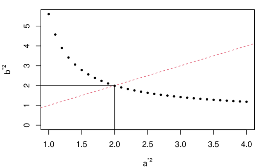
This means that collecting more information about the arm with mean response $\mu_{j}$ close to $\gamma_{j}$ implies a maximisation of the information gain $\Delta_{n_{j}}$. This property guarantees that the more valuable the learning about $\mu_{j}$, the higher the information gain associated to this arm. In addition, when $p\geq 1$, $\Delta_{n_{j}}$ is monotonically increasing with $\sigma_{j}$ (cfr. Figure 1b), reflecting the idea that the more the uncertainty around arm $j$ the more the learning value associated with sampling from it. When $\kappa\geq 0.5$, as more observations on arm $j$ are collected, the value of the information gain decreases, with higher values of $\kappa$ leading to a steeper decline of this function (cfr. Figure 1c).

For the desirable properties illustrated above, we suggest the use of the information gain in (6) as patient’s gain criterion to govern patients’ allocation in a sequential experiment.

Let $N_{j}$ be the total number of patients allocated to arm $j$ at the end of the trial and $N=\sum_{j=1}^{K}\,N_{j}$ the total number of patients treated at the end of the trial. The scheme to allocate the $N$ patients to the $K$ arms works as follows.

After a burn-in phase where an equal batch of $B\geq 1$ individuals is allocated to each of the $K$ arms, the $t$-th patient ($t=KB+1,\dots,N$) is allocated following the rule:

This rule may be seen as a deterministic response-adaptive criterion, where the next patient is almost surely allocated to the arm associated with the highest information gain. The algorithm proceeds until the total number of $N$ patients is attained. Finally, the arm $j^{*}$ whose final sample mean $\bar{x}_{N_{j}}$ is closest to the target is selected for the final recommendation; namely, $j^{*}=\underset{j=1,\dots,K}{\text{argmin}}\,|\bar{x}_{N_{j}}-\gamma_{j}|$. The burn-in phase is necessary to have a first estimate of the sample means of the $K$ arms, even more importantly when the sequential design is based on non-informative prior distributions.

The rule in (7) accounts for patient benefit by rewarding arms with mean responses closer to the target, while encouraging the exploration of arms with higher uncertainty. Notably, smaller values of $p$ tend to mitigate the impact that different values of the standard deviations have on the information gain, thus $p$ can be regarded as a parameter controlling the impact of the response variability on this information measure. Moreover, a too greedy algorithm may lead to an insufficient exploration of the alternative arms, resulting in poor performance in terms of statistical power (Villar et al., 2015). For this reason, a key role in the "exploration vs exploitation" trade-off is played by the parameter $\kappa$ which penalises an increasing number of observations on the same arm, offering more chances to other arms to be explored. Notably, a larger $\kappa$ corresponds to a higher penalisation of arms with many patients, favouring a more spread allocation. In Section 4, we show some strategies to select $\kappa$ in accordance with the trial objectives, while, in Section 5, we offer further insights on how this parameter affects the operating characteristics of the proposed design.

As alternative to (5), a weight function asymmetric around $\gamma_{j}$, allowing for a different weighting of values above and below the target, is discussed in Section B of the SM.

Let us now consider the case where $q>1$ endpoints are measured for each of the $K$ arms of a clinical trial. In addition, consider the $n_{j}$ responses from arm $j$ as an iid sequence of realisations of the $q\times 1$ random vectors $\bm{X}_{i_{1},\,j},\dots,\bm{X}_{i_{n_{j}},\,j}\overset{iid}{\sim}MVN(\bm{\mu}_{j},\,\bm{\Sigma}_{j})$, with mean vector $\bm{\mu}_{j}\in\mathbb{R}^{q}$ and covariance matrix $\bm{\Sigma}_{j}$ supposed to be known. Under these assumptions, an improper prior uniform on $\mathbb{R}^{q}$ for $\bm{\mu}_{j}$ will result in a posterior distribution $MVN(\bar{\bm{x}}_{n_{j}},\,\bm{\Sigma}_{n_{j}})$, where $\bar{\bm{x}}_{n_{j}}$ is the vector of sample means for the $j$-th arm and $\bm{\Sigma}_{n_{j}}=\frac{\bm{\Sigma}_{j}}{n_{j}}$. If $\bm{\Omega}_{n_{j}}=\bm{\Sigma}^{-1}_{n_{j}}$ is the posterior precision matrix, the posterior density of $\bm{\mu}_{j}$ is given by

Theorem 2 provides a closed-form expression for the information gain when a family of weight functions having a multivariate Gaussian kernel centered around the vector of target means $\bm{\gamma}_{j}$ is considered.

The proof is provided in Section A.2 of the SM. Interestingly, for $q=1$ the information gain in (10) coincides with the one in (6) with $p=2$. The information gain attains higher values in correspondence of vectors of the sample means being close to the vector of the target means, and it is also monotonically increasing with the variances of the endpoints (see section C.1 of the SM). The asymptotical behaviour of (10) is similar to the one of the information gain in (6), thus we consider $\kappa\geq 0.5$ for the same reasons argued for the univariate case.

In the bivariate case ($q=2$), the function in (10) can be expressed in scalar terms as

where $\bm{\gamma}_{j}=\bigr{(}\gamma_{j}^{\scriptscriptstyle(1)},\gamma_{j}^{\scriptscriptstyle(2)}\bigl{)}^{\prime}$, $\bar{\bm{x}}_{j}=\bigr{(}\bar{x}_{n_{j}}^{\scriptscriptstyle(1)},\bar{x}_{n_{j}}^{\scriptscriptstyle(2)}\bigl{)}^{\prime}$ and $\bm{\Sigma}_{j}=\biggl{(}\begin{smallmatrix}\sigma_{j}^{\scriptscriptstyle(11)}&\sigma_{j}^{\scriptscriptstyle(12)}\\ \\ \sigma_{j}^{\scriptscriptstyle(12)}&\sigma_{j}^{\scriptscriptstyle(22)}\end{smallmatrix}\biggr{)}$ with variances in the diagonal and covariance between the endpoints in the off-diagonal. The behaviour of the information gain as function of the correlation $\rho_{j}=\frac{\sigma_{j}^{\scriptscriptstyle(12)}}{\sqrt{\sigma_{j}^{\scriptscriptstyle(11)}\sigma_{j}^{\scriptscriptstyle(22)}}}$ is discussed in Section C.2 of the SM.

We adopt the function (10) as patients’ allocation criterion. As for the univariate case, the next patient of the sequential scheme is assigned to the arm with the highest information gain, while the arm selection is still based on the proximity between the final estimates of the means and the respective target mean values, i.e. the estimated best arm is the one whose final estimated mean vector is closest to the target vector.

We assume a generic context where a $K$-armed trial is considered and no control arm is adopted for comparison. Thus, $\binom{K}{2}$ pairwise comparisons may be necessary to test the superiority of an arm over the others, and this can be a computationally demanding task. Here, following the motivating trial and to be aligned with the final recommendation strategy, we propose a testing procedure which only compares the two best performing arms, by also taking into account their correct identification.

Let $j^{*}:=\underset{j=1,\dots,K}{\text{argmin}}\,|\mu_{j}-\gamma_{j}|$ be the best treatment arm and $j^{**}:=\underset{j=1,\dots,K,\,j\neq j^{*}}{\text{argmin}}\,|\mu_{j}-\gamma_{j}|$ be the second best treatment arm. In case of tie between two or more treatment arms, the best (or second best) arm is randomly determined among them. Denoting $\mu_{j^{*}}$ and $\mu_{j^{**}}$ the true mean responses of arm $j^{*}$ and arm $j^{**}$, respectively, we propose a test procedure which assesses whether $\mu_{j^{*}}$ is sufficiently much closer to the target $\gamma_{j}$ than $\mu_{j^{**}}$. Formally, we consider the following set of hypotheses:

If $\widehat{x}_{j}$ is the sample mean of arm $j$ at the end of the trial, the estimated best and second best arm are $\widehat{j}^{*}:=\underset{j=1,\dots,K}{\text{argmin}}\,|\widehat{x}_{j}-\gamma_{j}|$ and $\widehat{j}^{**}:=\underset{j=1,\dots,K,\,j\neq j^{*}}{\text{argmin}}\,|\widehat{x}_{j}-\gamma_{j}|$. The hypotheses in (11) are tested under a Bayesian framework where $H_{0}$ is rejected at a significance level $\alpha$ if the posterior probability that $|\mu_{\widehat{j}^{*}}-\gamma_{j}|<|\mu_{\widehat{j}^{**}}-\gamma_{j}|$ exceeds a fixed cut-off probability $\eta_{\alpha}$. Strategies to calibrate $\eta_{\alpha}$ to achieve type-I error control are proposed in Section 3.2.

However, comparing distances between the means of the two estimated best arms is not sufficient to make a claim on the true ones, thus we need to guarantee that the ground truth is correctly identified. For this reason, we propose two definitions of power incorporating their correct identification, under the assumption that $\mathbb{P}\bigl{(}\bigl{\{}\widehat{j}^{*}=j^{*},\,\widehat{j}^{**}=j^{**}\bigr{\}}\bigl{|}H_{0}\bigr{)}=1$.

The first proposal is to consider a conditional power,

where $\pi_{\widehat{j}^{*},\widehat{j}^{**}}$ is the posterior probability that $|\mu_{\widehat{j}^{*}}-\gamma_{j}|<|\mu_{\widehat{j}^{**}}-\gamma_{j}|$. Rejections of the null are counted in (12) only for pseudo-trials whose two best arms are correctly identified. Alternatively, one can consider a two-components power, namely

where correct identification is counted as a "success". Notice that $(1-\beta)_{TC}\leq(1-\beta)_{R}$.

Let us consider a wide set $\mathcal{S}_{0}=\{H_{0}^{(1)},\,\dots,H_{0}^{(S)}$} of plausible null scenarios, where $H_{0}^{(s)}$ is characterised by a particular vector of true mean responses. Given a specific design and a maximum tolerated type-I error probability $\alpha$, we define $\eta_{\alpha}^{(s)}$ as the individual cut-off value calibrated at level $\alpha$ under the null scenario $H_{0}^{(s)}$ ($s=1,\dots,S)$, namely a threshold value $\eta_{\alpha}^{(s)}$ such that $\mathbb{P}\Bigl{(}\pi_{\widehat{j}^{*},\widehat{j}^{**}}>\eta_{\alpha}^{(s)}\Bigl{|}\,H_{0}^{(s)}\Bigr{)}=\alpha$. Notice that, for a fixed $\eta_{\alpha}^{(s)}$, this probability can be efficiently evaluated via Monte Carlo simulations.

To guarantee a strong control of the type-I error, one can fix the threshold $\eta_{\alpha}$ to the maximum of the individual cut-off probabilities, i.e. $\eta_{\alpha}^{\text{max}}=\underset{s=1,\dots,S}{\max}\,\eta_{\alpha}^{(s)}$. This is a conservative strategy which assures that the probability of incorrectly detecting the presence of a superior arm under the null does not exceed $\alpha$ in each of the scenarios in $\mathcal{S}_{0}$. Ideally, $\mathcal{S}_{0}$ should contain a wide variety of scenarios in order to control as many situations as possible. In practice, there may be scenarios which are thought to be highly unlikely and can be ruled out. As rule of thumb, we suggest to consider null scenarios with $\mu_{j}$ not being distant from $\gamma_{j}$ more than $10$ times the largest standard deviation. Remember that for normal responses it is known that the response $X_{j}$ will be in the interval $\mu_{j}\pm 3\sigma_{j}$ with probability higher than $0.97$. Thus, a distance $|\mu_{j}-\gamma_{j}|$ much higher than $3\sigma_{j}$ would imply that values in the neighbourhood of $\gamma_{j}$ are very unlikely for arm $j$. Furthermore, in some contexts, null scenarios with distances larger than $10\cdot\max_{j}\sigma_{j}$ might signify the ineffectiveness of all the treatments and, therefore, having a control on any of them may be out of the trial scope.

In some cases, the strong control of the type-I error may be a too stringent requirement which leads to a loss of power. This is even more evident when there are only few scenarios requiring a substantially higher cut-off value than the rest. Similarly to Daniells et al. (2024), we propose to relax the required type of control, trying to reach an average control of the type-I error probability rather than a strong one. Then the resulting threshold value is $\eta_{\alpha}^{\text{ave}}$ such that $\frac{1}{S}\sum_{s=1}^{S}\,\alpha^{(s)}=\alpha$, where $\alpha^{(s)}$ is the individual type-I error probability associated with scenario $H_{0}^{(s)}$. In this case, $\alpha$ can be regarded as the average type-I error probability for the set of scenarios in $\mathcal{S}_{0}$. Notice that the simple average can be replaced by a weighted average, giving larger weight to scenarios which are more relevant than others.

The choice of the penalisation parameter $\kappa$ is crucial since to control the trade-off between exploration and exploitation. We consider as "optimal", a value of $\kappa$ which maximises a specific operating characteristic of interest (e.g. statistical power, percentage of times the best arm is selected in repeated trials). The optimal value of $\kappa$ depends on several parameters, like the vector of true means, the vector of standard deviations, the vector of target means, the total sample size, the number of arms, the burn-in size and the parameter $p$. Apart from the vectors of the true means and true standard deviations, we suppose that all the other parameters are fixed in advance by clinicians. Particular caution must be placed on the vector of standard deviations which may be supposed to be either known (i.e. prior guess used as estimate) or unknown.

Following Mozgunov and Jaki (2020b), we discuss a general approach to select the robust optimal value of $\kappa$ which does not require the prior knowledge on the mean responses and the standard deviations. The idea is to consider a large variety of plausible alternative scenarios, each one characterised by a vector of mean responses (and a vector of standard deviations, in case they are assumed to be unknown), and to select the value of $\kappa$ associated with the average best performance over all the considered scenarios.

In practice, one considers a set $\mathcal{S}_{1}=\{H_{1}^{(1)},\,\dots,H_{1}^{(S)}\}$ of $S$ plausible alternative scenarios, where $H_{1}^{(s)}$ is characterised by the set of unknown parameters, and a grid of values for $\kappa$. Then, the algorithm to find the robust optimal $\kappa$ consists in the following steps:

1. 1.

   Define an objective function $g(u^{(s)}(\kappa))$, where $u^{(s)}(\kappa)$ is the value assumed by a particular operating characteristic of interest for a fixed $\kappa$ and scenario $s$ ($s=1,\dots,S$).

2. 2.

   Compute $u^{(s)}(\kappa)$, for each scenario $s$ and value of $\kappa$ in the considered grid.

3. 3.

   Find the optimal $\kappa$: $\kappa^{*}=\text{argmin}_{\kappa}\,\frac{1}{S}\sum_{s=1}^{S}\,g(u^{(s)}(\kappa))$.

Averaging over a wide set of scenarios offers a robust way to select a suitable value of $\kappa$ regardless of the true values of the parameters: although the optimal value of $\kappa$ may not be convenient for some particular scenario, this procedure ensures that it is nearly optimal.

The objective functions should be chosen in accordance with the operating characteristic that one wants to target in the calibration of $\kappa$. If the main objective is to maximise the patient benefit (PB), we propose to target the average percentage of experimentation of the best arm (evaluated over $M$ pseudo-trials), namely

where $a_{tm}=j^{*}$ if and only if patient $t$ is allocated to the true best arm $j^{*}$ during the pseudo-trial $m$. Supposing that $u_{1}(\kappa)=(PB)_{\kappa}$ for any $\kappa$, we adopt the following squared difference as corresponding objective function:

quantifying how far each value $u^{(s)}_{1}(\kappa)$ is from $u^{(s)}_{\text{max}}=\max_{k}u_{1}^{(s)}(\kappa)$.

In case the objective is to achieve a pre-specified level of power, than we use

where $u_{2}^{(s)}(\kappa)$ is either the power defined in (12) or in (13), $u^{(s)}_{2,FR}$ is the power attained using fixed and equal randomisation (FR) and $\xi\in[0,1]$. The optimal $\kappa$ will be then the smallest $\kappa$ for which the probability to obtain a power higher than $80\%$ of the power attained by the FR is at least $\xi$. This avoids a too excessive penalisation of increasing arm sample sizes, once that the requirement in terms of power is met.

Let us consider an early Phase IIa proof-of-concept oncology clinical trial such as the one introduced in the motivating example of Section 1. We consider $K=4$ alternative treatments (no control arm) and a total of $N=100$ patients recruited at the end of the trial. We assume that the primary endpoint is PD-marker measured on a continuous scale, and responses from arm $j$ closer to the target $\gamma_{j}$ ($j=1,\dots,K$) are more desirable. For simplicity, we assume $\gamma_{j}=\gamma=0$ for $j=1,\dots,K$, implying that sample means equal to $\epsilon$ and $-\epsilon$ ($\epsilon>0$) are treated equally by our proposed design. Thus, for a given scenario, the best treatment arm is the one associated with smallest mean response in absolute value.

We investigate the performance of our method over $S=500$ random scenarios under the alternative hypothesis in (11). Each scenario is characterised by a vector of means $(\mu_{1},\dots,\mu_{K})$, where $\mu_{j}$ is generated from a $Unif[-4,4]$, $\forall j=1,\dots,K$, while variances are assumed to be known and equal to $\sigma_{j}^{2}=2^{2}$, $j=1,2,3$, $\sigma_{4}^{2}=4^{2}$ for each scenario. Details and a full analysis for the case of unknown variances are presented in Section F of the SM.

Operating characteristics of interest are (i) the type-I error rates in correspondence of specific null scenarios, (ii.a) conditional ($(1-\beta)_{C}$) and (ii.b) two-components ($(1-\beta)_{TC}$) statistical power (cfr. Section 3.1), (iii) the average percentage of experimentation of the best arm - cfr. (14) - as measure of patient benefit (PB) and (iv.a) the percentage of pseudo-trials with correct identification of the best arm (CS${}_{I}(\%)$) and of (iv.b) the two best arms (CS${}_{I\&II}(\%)$). For each given scenario, operating characteristics are assessed over $M=10^{4}$ pseudo-trials (Monte Carlo simulations).

In the following, we will denote WE($p$,$\kappa$) the class of designs proposed in Section 2.2, and we will consider the case of $p=\{1,\,2\}$: this will offer insights on how different degrees of discrimination between arm-specific variances affect the resulting operating characteristics.

We compare its performance with several alternative allocation procedures which have good properties either in terms of statistical power or patient benefit. For a fair comparison with our proposal and to narrow down the set of competitors, we restrict to response-adaptive designs based on deterministic allocation rule. Additionally, in line with the objective of the trial, we only consider those adaptive designs that try to skew allocations in favour of arms with means closer to the target. Specifically, we compare with the following designs: (i.) Fixed and equal randomisation (FR), where each patient can be treated in a specific arm with fixed probability $\frac{1}{K}$; (ii.) Current belief (CB), where the next patient is treated in the arm with posterior mean $\bar{x}_{n_{j}}$ closest to the target $\gamma_{j}$; (iii.) Thompson Sampling (TS), where patient $t$ is treated in the arm which maximises the adjusted posterior probability of being the best, i.e. $\pi_{j}=\frac{\mathbb{P}(j=j^{*}|\texttt{data})^{c}}{\sum_{l=1}^{K}\,\mathbb{P}(l=j^{*}|\texttt{data})^{c}}\,,$ where $c=\frac{t}{2N}$ helps to stabilise the resulting allocations; (iv.) Symmetric Gittins Index (SGI) and (v.) Targeted Gittins Index (TGI), two modifications of Smith and Villar (2018)’s proposal involving $\gamma_{j}$ (full details are provided in Section D of the SM). We use objective priors and fix $d=0.99$, in line with the considerations of Wang (1991) and Williamson and Villar (2020) for a trial of size $N=100$. Notice that, apart from FR, all the alternative designs can be classified as response-adaptive. FR is taken as benchmark for power comparison, due to its even exploration of all the arms and its wide application in real trials. CB and TS are common and intuitive response-adaptive designs, which are generally associated with good performance in terms of patient benefit. Finally, SGI and TGI are modifications of a forward-looking design which is oriented toward a patient benefit objective (Smith and Villar, 2018; Williamson and Villar, 2020).

In absence of prior knowledge about the treatments, the burn-in size is fixed to $B=5$ for all the response-adaptive designs to help sequential algorithms collecting sufficient preliminary information about all the arms. The same burn-in size is chosen for both the case of known and unknown variances, in order to isolate its effect in the comparison between these two settings. Further details are provided in Section E.1 of the SM.

For a given combination of $p$ and $\kappa$, we calibrate design-specific cut-off probabilities under the set of null scenarios $\mathcal{S}_{0}=\bigl{\{}(\mu_{1},\dots,\mu_{K}):\,\mu_{j}-\gamma=c,\,c\geq 0,\,\forall j\bigr{\}}$ both considering the strong and the average control of the type-I error at a level $\alpha=5\%$. Two types of considerations should be made on this choice of null scenarios: (i) calibration is done under the most challenging situation where there is no sub-optimal arm; (ii) one only considers $c\geq 0$ since, for $\gamma=0$, values $c$ and $-c$ are treated equally in the definition of best arm. Details on the choice of the null scenarios are presented in Section E.2 of the SM.

Response-adaptive designs tend to be associated with higher type-I error probabilities when $c$ is small, while FR design is associated with type-I error rates which increase with $c$ before reaching a plateau. This different behaviour can be explained by the peculiar nature of response-adaptive designs. Indeed, variability around the arm responses can overly penalise some arms at the beginning of the trial in favour of others. Notably, when $c$ is very small (i.e. all true means are very close to the target value), most of the patients are likely to be assigned to the arm which - by chance - performs better at the beginning of the trial: as a result, any other arm may not have the chance to be further explored, thus being falsely identified as inferior at the end of the trial. If a practitioner aims at reducing even more the resulting inflation of the type-I error rate associated with response-adaptive designs in this type of scenarios, a possible solution is to consider higher burn-in sizes (cfr. Section E.1 of the SM), possibly at the expense of a lower patient benefit: although a larger $B$ is associated to a more exhaustive exploration of all the arms and to more precise estimates, a too high value may lead to assign a high percentage of patients to sub-optimal treatment arms.

The implementation of the proposed design requires to fix in advance the penalisation parameter $\kappa$. We apply the procedure presented in Section 4 both for the objective function maximising the patient benefit and the one achieving a specific level of statistical power.

We perform two independent analyses for the case of $p=1$ and $p=2$. After preliminary checks, the sequence of values for $\kappa$ is restricted in the interval [$0.5$, $1.5$] with step $0.05$. For the power objective function, we require that $80\%$ of the power of the FR is achieved with probability higher or equal to $\xi=0.9$. This condition should assure that in most of the scenarios the resulting power is not too below the one achieved by the FR design. As a measure for $u_{2}(\kappa)$, we consider the two-components power defined in (13) with design-specific cut-off probabilities guaranteeing an average control of the type-I error rate at $\alpha=5\%$ over the set of scenarios considered in Section 5.2.

As anticipated, lower values of $\kappa$ are suggested when the criterion optimises the patient benefit, while larger values of $\kappa$ are necessary to achieve the power objective. At the same time, higher values of $p$ requires higher values of $\kappa$ to attain the specific objective to compensate the higher relevance attributed to the variance. Therefore, the value of $\kappa=0.55$ and $\kappa=0.8$ will be used when $p=1$, while $\kappa=0.7$ and $\kappa=1.1$ when $p=2$.

WE designs achieve good performance in terms of patient benefit and identification of the best arm than their competitors, with WE($1$, $0.8$) and WE($2$, $1.1$) achieving a power almost comparable to FR. The even exploration of all the arms which characterises FR also leads to a higher percentage of correct identification of the two best arms, but with high variability across the scenarios. CB and TS generally perform worse than the other response-adaptive designs: notably, they both achieve high medians in terms of patient benefit but with high variability around them. In contrast, SGI and WE($1$, $0.55$) achieve comparable patient benefit measures, but with much less variability around their medians.

To further investigate the performance of our proposal, we pick two scenarios from the ones considered in Figure 4. Notably, given $\bm{\sigma}=(2,2,2,4)$ and $\gamma_{j}=0\,\forall j$, we consider: (i) Scenario I, characterised by $\bm{\mu}=(1.91,-3.36,-0.37,3.99)$, with the worst treatment arm having the highest variability; (ii) Scenario II, characterised by $\bm{\mu}=(1.13,-3.48,-3.57,0.34)$, with the best treatment arm having the highest variability. Table 1 illustrates the operating characteristics of the considered designs under Scenario I and II.

Under Scenario II, WE($2$, $0.65$) and WE($2$, $1.2$) achieve the highest value of PB, but the second one is associated with lower variability around this measure and, thus, can be deemed to be more reliable. CB performs best in terms of conditional power compared to the other designs, but fails in correctly identify the best treatment more than $50\%$ of the times. In contrast, WE designs correctly identifying the two best arms in a high percentage of replicas (i.e. more than $75\%$) and are associated with higher values of two-components power. Notice that FR is associated with a much lower power than the other designs, probably due to the relatively lower exploration ($25$ patients on average) of the best arm.

Overall, the considered WE designs performance are comparable to the ones of the other response-adaptive designs, with small differences in terms of patient benefit but larger gain in terms of correct identification of the best arm and two-components power. In addition, WE designs generally tend to achieve a much higher patient benefit than FR due to their ability to skew allocations according to the accrued data, at the cost of moderately lower power. With a selection of $\kappa$ targeting the power, WE can result in a statistical power closer to the one of FR, but with remarkably larger values of PB. Finally, when the best arm has also the most variable response, the flexibility of WE designs allows it to achieve an even higher gain over FR in terms of power. Further details on how operating characteristics are affected by different choices of $p$ and $\kappa$ are given in Section E.3 of the SM.

In Section 6, we focused on a single quantitative endpoint. However, multiple endpoints are generally collected in clinical trials and we can adopt the design proposed in Section 2.3 to deal with this particular context. In particular, we illustrate the performance of the novel response-adaptive design in the case of an oncology clinical trial with $K=4$ competing drug combinations, a total sample size of $N=100$ and two co-primary endpoints. The first endpoint is a PD-marker (PDM) - e.g., see motivating setting in Section 1 - targeting a specific value $\gamma_{j}^{(1)}=\gamma^{(1)}=0$, for all $j=1,\dots,K$, while the second endpoint is the tumour shrinkage rate (TSR, $\%$) whose theoretical target is assumed to be $\gamma_{j}^{(2)}=\gamma^{(2)}=100$ (i.e. full disappearance of the tumour), for all $j=1,\dots,K$. Variance matrices are assumed to be known and equal to $\bm{\Sigma}_{j}=\Big{(}\begin{smallmatrix}2^{2}&0\\ 0&8^{2}\end{smallmatrix}\Big{)},\,\forall j$. The goal of the study is to identify the best arm, to claim its superiority and to allocate most of the patients to it during the trial.

As illustration, we consider the design for bivariate endpoints described in Section 2.3 with $\kappa=\{0.5,\,0.75\}$. We compare its performance to two alternative approaches: (a.) fixed and equal randomisation (FR), (b.) current belief (CB). As already discussed in Section 5, FR is expected to achieve high power due to the even exploration of all the arms, while CB is expected to result in high PB. We choose a burn-in size of $B=1$ patient per arm for response-adaptive designs, and we consider a scenario where $\bm{\mu}^{(1)}=(1,-1,2,-2.5)^{\prime}$ and $\bm{\mu}^{(2)}=(10,25,55,60)^{\prime}$. The four treatment arms can be characterised as follows: the first two treatments have values of the PDM relatively close to the target but associated with a relatively small TSR ($10\%$ and $25\%$, respectively); the third has twice the PDM of the first but it is associated with a remarkable average TSR (i.e. $55\%$); finally, the fourth is associated with a slightly poorer average PDM (e.g. more distant from the target) than the third treatment, but it has the highest average TSR. Observe that coefficients of variation of the PDM are relatively small (range: 0.5-1.25) if compared with the ones of TSR (1.25-7.5).

The definition of "best" arm in the bivariate case may be more challenging, and it strictly depends on the adopted distance. The means of the two endpoints can vary greatly in magnitude, and the use of a Minkowski distance (e.g. Euclidean, Manhattan) may lead to the endpoint with higher magnitude prevailing over the others, unless some sort of standardisation is applied. Notably, for a given arm $j$, we propose to use a standardised version of the distance between the target vector and the true mean vector, i.e. $\widetilde{d}(\bm{\mu}_{j},\bm{\gamma}_{j})=\sum_{l=1}^{2}\frac{\bigl{|}\mu_{j}^{\scriptscriptstyle(l)}-\gamma_{j}^{\scriptscriptstyle(l)}\bigr{|}}{\sqrt{\sigma_{j}^{\scriptscriptstyle(ll)}}}\,.$ Therefore, the final recommendation is $\widehat{j}^{*}:=\underset{j=1,\dots,K}{\text{argmin}}\,\widetilde{d}(\bm{\mu}_{j},\bm{\gamma}_{j})$. Adopting this standardised distance, the fourth treatment arm can be regarded as the best one.

We consider the same operating characteristics as in Section 5 to assess the performance of the considered designs. Hypothesis testing is performed following the same procedure described for the univariate case (cfr. Section 3), with the only exception that $H_{0}$ is rejected at significance level $\alpha$ if the posterior probability that $\widetilde{d}(\bm{\mu}_{\hat{j}^{*}},\,\bm{\gamma}_{j})<\widetilde{d}(\bm{\mu}_{\hat{j}^{**}},\,\bm{\gamma}_{j})$ exceeds the cut-off probability $\eta_{\alpha}$, where $\hat{j}^{*}$ and $\hat{j}^{**}$ are, respectively, the estimated best and second best treatment arms according to distance $\widetilde{d}(\cdot)$.

The calibration under strong control is available in Section G of the SM. Notably, FR and WE designs are associated with individual type-I error rates which do not exceed $6\%$, with the exception of WE(0.5) which registers a $9\%$ type-I error rate under the configuration $\bm{c}=(0,\,75)^{\prime}$. FR and WE(0.75) have more conservative type-I error rates when the mean of PDM endpoint equals the target in all the treatment arms. On the contrary, there is a large inflation of type-I error rate of CB in correspondence of these scenarios, while elsewhere it is below $5\%$.

References

- Antognini and Giovagnoli [2010] Alessandro Baldi Antognini and Alessandra Giovagnoli. Compound optimal allocation for individual and collective ethics in binary clinical trials. Biometrika, 97(4):935–946, 2010.
- Bartroff and Leung Lai [2011] Jay Bartroff and Tze Leung Lai. Incorporating individual and collective ethics into phase i cancer trial designs. Biometrics, 67(2):596–603, 2011.
- Azriel et al. [2012] David Azriel, Micha Mandel, and Yosef Rinott. Optimal allocation to maximize the power of two-sample tests for binary response. Biometrika, 99(1):101–113, 2012.
- Thall et al. [1989] PF Thall, R Simon, and SS Ellenberg. A two-stage design for choosing among several experimental treatments and a control in clinical trials. Biometrics, 45(2):537–547, 1989.
- Rosenberger and Lachin [1993] William F Rosenberger and John M Lachin. The use of response-adaptive designs in clinical trials. Controlled clinical trials, 14(6):471–484, 1993.
- Berry and Eick [1995] Donald A Berry and Stephen G Eick. Adaptive assignment versus balanced randomization in clinical trials: a decision analysis. Statistics in medicine, 14(3):231–246, 1995.
- Robertson et al. [2023] David S Robertson, Kim May Lee, Boryana C López-Kolkovska, and Sofía S Villar. Response-adaptive randomization in clinical trials: from myths to practical considerations. Statistical science: a review journal of the Institute of Mathematical Statistics, 38(2):185, 2023.
- Rombach et al. [2020] Ines Rombach, Ruth Knight, Nicholas Peckham, Jamie R Stokes, and Jonathan A Cook. Current practice in analysing and reporting binary outcome data—a review of randomised controlled trial reports. BMC medicine, 18:1–8, 2020.
- Altman and Royston [2006] Douglas G Altman and Patrick Royston. The cost of dichotomising continuous variables. Bmj, 332(7549):1080, 2006.
- Zhao et al. [2015] Xuemei Zhao, Vijay Modur, Leonidas N Carayannopoulos, and Omar F Laterza. Biomarkers in pharmaceutical research. Clinical chemistry, 61(11):1343–1353, 2015.
- Kaiafa et al. [2021] Georgia Kaiafa, Stavroula Veneti, George Polychronopoulos, Dimitrios Pilalas, Stylianos Daios, Ilias Kanellos, Triantafyllos Didangelos, Stamatina Pagoni, and Christos Savopoulos. Is hba1c an ideal biomarker of well-controlled diabetes? Postgraduate medical journal, 97(1148):380–383, 2021.
- Kelbert and Mozgunov [2015] Mark Yakovlevich Kelbert and Pavel Mozgunov. Asymptotic behaviour of the weighted renyi, tsallis and fisher entropies in a bayesian problem. Eurasian Mathematical Journal, 6(2):6–17, 2015.
- Suhov et al. [2016] Yuri Suhov, Izabella Stuhl, Salimeh Yasaei Sekeh, and Mark Kelbert. Basic inequalities for weighted entropies. Aequationes mathematicae, 90:817–848, 2016.
- Kasianova et al. [2021] Ksenia Kasianova, Mark Kelbert, and Pavel Mozgunov. Response adaptive designs for phase ii trials with binary endpoint based on context-dependent information measures. Computational Statistics & Data Analysis, 158:107187, 2021.
- Mozgunov and Jaki [2020a] Pavel Mozgunov and Thomas Jaki. Improving safety of the continual reassessment method via a modified allocation rule. Statistics in medicine, 39(7):906–922, 2020a.
- Kasianova et al. [2023] Ksenia Kasianova, Mark Kelbert, and Pavel Mozgunov. Response-adaptive randomization for multiarm clinical trials using context-dependent information measures. Biometrical Journal, 65(8):2200301, 2023.
- Mozgunov and Jaki [2019] Pavel Mozgunov and Thomas Jaki. An information theoretic phase i–ii design for molecularly targeted agents that does not require an assumption of monotonicity. Journal of the Royal Statistical Society Series C: Applied Statistics, 68(2):347–367, 2019.
- Mozgunov and Jaki [2020b] Pavel Mozgunov and Thomas Jaki. An information theoretic approach for selecting arms in clinical trials. Journal of the Royal Statistical Society Series B: Statistical Methodology, 82(5):1223–1247, 2020b.
- Azriel et al. [2011] David Azriel, Micha Mandel, and Yosef Rinott. The treatment versus experimentation dilemma in dose finding studies. Journal of Statistical Planning and Inference, 141(8):2759–2768, 2011.
- Villar et al. [2015] Sofia Villar, Jack Bowden, and James Wason. Multi-armed bandit models for the optimal design of clinical trials: Benefits and challenges. Statistical Science, 30:199–215, 2015.
- Aziz et al. [2021] Maryam Aziz, Emilie Kaufmann, and Marie-Karelle Riviere. On multi-armed bandit designs for dose-finding trials. Journal of Machine Learning Research, 22(14):1–38, 2021.
- Smith and Villar [2018] Adam L Smith and Sofía S Villar. Bayesian adaptive bandit-based designs using the gittins index for multi-armed trials with normally distributed endpoints. Journal of applied statistics, 45(6):1052–1076, 2018.
- Williamson and Villar [2020] S Faye Williamson and Sofía S Villar. A response-adaptive randomization procedure for multi-armed clinical trials with normally distributed outcomes. Biometrics, 76(1):197–209, 2020.
- Daniells et al. [2024] Libby Daniells, Pavel Mozgunov, Helen Barnett, Alun Bedding, and Thomas Jaki. How to add baskets to an ongoing basket trial with information borrowing. arXiv preprint arXiv:2407.06069, 2024.
- Wang [1991] You-Gan Wang. Sequential allocation in clinical trials. Communications in Statistics-Theory and Methods, 20(3):791–805, 1991.
- Ghosh [2011] Malay Ghosh. Objective priors: An introduction for frequentists. Statistical Science, 26(2):187–202, 2011.
- Shi and Yin [2019] Haolun Shi and Guosheng Yin. Control of type i error rates in bayesian sequential designs. Bayesian Analysis, 14(2):399–425, 2019.
- Liu et al. [2009] Guohui Liu, William F Rosenberger, and Linda M Haines. Sequential designs for ordinal phase i clinical trials. Biometrical Journal: Journal of Mathematical Methods in Biosciences, 51(2):335–347, 2009.
- Russo [2020] Daniel Russo. Simple bayesian algorithms for best-arm identification. Operations Research, 68(6):1625–1647, 2020.
- Jourdan et al. [2022] Marc Jourdan, Rémy Degenne, Dorian Baudry, Rianne de Heide, and Emilie Kaufmann. Top two algorithms revisited. Advances in Neural Information Processing Systems, 35:26791–26803, 2022.
- Wang and Tiwari [2023] Jixian Wang and Ram Tiwari. Adaptive designs for best treatment identification with top-two thompson sampling and acceleration. Pharmaceutical Statistics, 22(6):1089–1103, 2023.
- Gittins et al. [2011] John Gittins, Kevin Glazebrook, and Richard Weber. Multi-armed bandit allocation indices. John Wiley & Sons, 2011.
Supplementary Material
A Proofs
A.1 Proof of Theorem 1
Proof.
Consider the generic arm . It is well known that the Shannon entropy of a normal distribution with mean and variance is given by
while the weighted Shannon entropy depends on the adopted weight function.
To begin, one can derive the explicit formula of the (normalised) weight function. For this purpose, the following equation is useful: