A quantitative Birman-Menasco finiteness theorem and its application to crossing number
Abstract.
Birman-Menasco proved that there are finitely many knots having a given genus and braid index. We give a quantitative version of Birman-Menasco finiteness theorem, an estimate of the crossing number of knots in terms of genus and braid index. This has various applications of crossing numbers, such as, the crossing number of connected sum or satellites.
1. Introduction
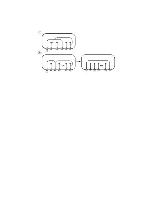
In [7] Birman-Menasco proved (in)finiteness theorem on closed braid representatives of knots and links; a knot or link has only finitely many closed braid representatives, up to conjugacy and exchange move. Here an exchange move is an operation that converts an -braid of the form () to a braid and its converse (see Figure 1). As a byproduct they proved another remarkable finiteness result;
Theorem 1 (Birman-Menasco finiteness theorem [7]).
For given , there are only finitely many knots/links with genus and braid index .

In this paper, we give a quantitative version of Theorem 1, an estimate of the crossing number by braid index and genus. For a link in , let and be the braid index, the minimum crossing number, and the maximum euler characteristic of Seifert surface, respectively.
Theorem 2 (Quantitative Birman-Menasco finiteness theorem).
Let
For a link in ,
holds.
The case is easy and the case is proven in [13] by using a special property of closed 3-braid that a closed 3-braid always bounds a minimum genus Bennequin surface, a minimum genus Seifert surface whose braid foliation has only aa-singular points [1, 5].
In the following, we restrict our attention to knots, and use the knot genus instead of the maximum euler characteristic.
Theorem 2 implies that is a linear approximation of the crossing number. This has several applications to the crossing numbers since the genus is one of the most familiar and well-studied invariant whereas the minimum crossing number is one of the most difficult invariant whose basic properties are still unknown.
It is a famous conjecture that [14, Problem 1.65]. Theorem 2 immediately gives an estimate of the crossing number of composite knots.
Corollary 1.
For a knot in let .
Proof.
Recall that is additive under connected sum, and that is also additive under connected sum [6]. Thus
∎
In [15] Lackenby showed that . Although the estimate given in Corollary 1 gets worse as increases, when is small it gives a better estimate.
Our proof gives an estimate of regularity introduced in [18] which plays an important role to relate two different problem; a genericity of hyperbolic knots/links and the additivity of crossing numbers.
Definition 3.
For , a knot is -regular if if contains as its prime factor.
Corollary 2.
For a knot in , is -regular.
Similarly, we have an estimate of the crossing number of satellite knots and an estimate of the asymptotic crossing number. The asymptotic crossing number of is defined by111The definition of the asymptotic crossing number given here is a version appeared in Kirby’s problem list [14]. In [8] Freedman-He called this the quadratic asymptotic crossing number and use different definition for the assymptotic crossing number, which we denote by . Since Freedman-He proved , the inequality in Corollary 3 is valid for .
where the infimum is taken over all satellites of with winding number . It is conjectured [14, Problem 1.68].
Corollary 3.
Let be a satellite knot with companion knot and pattern , whose winding number (homological degree) is . Then
In particular,
Proof.
Although Corollary 3 is meaningful only if is small compared with , it gives a linear lower bound of in terms of .
A famous satellite crossing number conjecture asserts [14, Problem 1.67]. Corollary 3 says that the satellite crossing number conjecture is true when and are large enough compared with .
A weaker and more tractable version of the satellite crossing number conjecture, for the -cable of which we call the cabling crossing number conjecture, is still open. For a braided -cable, a satellite knot whose pattern is a closed -braid in the solid torus, we have another estimate that gives more supporting evidences for the cabling crossing number conjecture and the satellite crossing number conjecture which works even if is large;
Corollary 4.
If is a braided -cable of , then
Thus, if then .
Proof.
In particular, since , the cabling crossing number conjecture is true for closed 3-braids:
Corollary 5.
If then for all -cables of .
It is interesting to ask whether Corollary 4 can be extended to general satellite knot. We used the braided -cable assumption is to guarantee . It looks to be reasonable to expect for satellite of with winding number so the same conclusion as Corollary 4 holds for general satellite knot with winding number .
In [16] Lackenby showed if is a satellite of . Since this estimate uses an estimate for -cable of of and Corollary 4 gives an improvement of Lackenby’s estimate [16, Theorem 5.1], one can improve Lackenby’s bound when is not so large. Indeed, combining Lackenby’s another result and our result we give a dramatic improvement of the estimate of the crossing number of satellite knots when is not large.
Corollary 6.
If is a satellite of ,
Proof.
Finally we give another application. The braid index problem is a problem to algorithmically compute the braid index of a link from a given diagram of . Strictly speaking, to make it as a decision problem, by the braid index problem we mean the problem to determine, for a given diagram of and a natural number , determine whether or not. Since is the unknot if and only if , this problem includes the unknotting problem, a problem to recognize the unknot.
Theorem 4.
The braid index problem is solvable.
Proof.
Our proof of Theorem 2 actually shows that a link has a closed -braid diagram that has at most crossings. There are finitely many closed -braid diagram with less than or equal to crossings. Since one can effectively enumerate such closed braid diagrams, by checking all the possibilities (this is possible since one can algorithmically check a given diagram represents or not [9, 10, 11]) one can determine or not algorithmically. ∎
It is desirable to give more direct algorithm of the braid index problem that avoids to use knot recognition, in a spirit of the Birman-Hirsch unknotting algorithm [3]. Also, it is an interesting problem to determine the computational complexity of the braid index problem.
Acknowledgement
The author has been partially supported by JSPS KAKENHI Grant Number 19K03490,16H02145. He would like to thank Joan Birman for stimulating comments for earlier version of the paper, and would like to thank to Sorsen Rebecca and Keiko Kawamuro pointing out an error in the earlier version of the paper.
2. Proof of Theorem 2
2.1. Quick review of braid foliation
In this section we briefly review Birman-Menasco’s braid foliation techniques. For details of braid foliation theory, we refer to [17] or [2].
Let be the unknot in and fix a fibration whose fiber is a disk bounded by . An oriented link is a closed -braid with axis if positively transverse to every fiber at points.
Let be an oriented incompressible Seifert surface of a closed -braid . We put so that induces a singular foliation of satisfying the following properties;
-
(i)
and transversely intersect. Moreover, each is an elliptic singular point of ; there is a disk neighborhood of in such that the foliation on is the radial foliation with node .
-
(ii)
All but finitely many fibers transversely intersect with . Each exceptional fiber is tangent to at exactly one point in the interior of , as a saddle tangency that appears as a hyperbolic singular point of .
-
(iii)
Each leaf of , a connected point of , transverse to .
We call the foliation satisfying these properties braid foliation.
An elliptic singular point is positive (resp. negative) if the sign of intersection of at is positive (resp. negative). A hyperbolic singular point is positive (resp. negative) if the positive normal direction of at agrees (resp. desagrees) with that of at (see Figure 2)222Although in the following argument the sign of hyperbolic point does not appear explicitly, it plays a crucial role in the proof of Proposition 1 below..

If a connected component of is a simple closed curve, it bounds a disk in . Since is incompressible, by standard innermost circle argument one can remove such leaves by isotopy of . Thus in the following, we always assume that the leaf of is either
-
•
a-arc: an arc connecting a positive elliptic point and a point of , or,
-
•
b-arc: an arc connecting two elliptic points of opposite signs.
Moreover, with no loss of generality, we may assume that each b-arc in is essential as a properly embedded arc in the punctured disk . In other words, both components of are pierced by the braid .
According to the types of nearby leaves, hyperbolic points of are classified into three types, , and and each hyperbolic point has a canonical foliated neighborhood as shown in Figure 3 which we call -tile, -tile, and -tile.

A decomposition of into tiles induces a cellular decomposition of ; The -cells are tiles, the -cells are -arcs and -arcs that appear as the boundary of tiles, and the -cells are elliptic points and the end points of -arc 1-cells.
2.2. Euler characteristic equality
We say that an elliptic point is of type if the valence is and it is a boundary of -arc 1-cells and -arc -cells. We denote by be the number of elliptic points of type .
By a standard euler characteristic counts we have the following equality which we call the euler characteristic equality, or, the fundamental equality of braid foliation;
| (2.1) | ||||
The following result plays the fundamental role in the braid foliation theory and explain why exchange move is a fundamental operation in braid foliation; using exchange move one can simplify the braid foliation (or braid itself, by destabilization) so that it contains no low-valency vertices. In a light of the euler characteristic equality (2.1), this gives a strong constraint for .
Proposition 1.
[7, Lemma 4] If , by applying exchange move we may assume that .
2.3. Braid foliation and crossing number
One can read the braid from the braid foliation [3, 4, 12]; one -tile gives rise to a braid of the form
and one -tile gives rise to a braid of the form,
A bb-tile does not affect the boundary the braid .
One useful way to see this is to use a movie presentation, a sequence of slice that describes how the arcs in changes as increase as we illustrate in Figure 4.

Let and be the number of and tiles in the braid foliation, respectively. Since the above discussion shows that one aa-tile provides a braid with at most crossings and one ab-tile provides a braid with at most crossings, we have an estimate of the crossing number via the braid foliation
With a little more argument we slightly improve the estimate as follows;
Proposition 2.
Let be a closed -braid and be an incompressible Seifert surface admitting a braid foliation.
-
(i)
If then
-
(ii)
If then
Proof.
(i): Assume that . Then case is obvious so we assume that . Let be the number of aa-tiles that gives rise to a braid and let . Here indices are understood by modulo so we regard as . Since
by taking conjugates we may assume that . Thus . Each ab-tile counted in provides a braid with one crossing. Each of rest of the aa-tiles provides a braid with at most crossings so
(ii) When , the braid foliation of contains at least one negative elliptic point. We put a negative elliptic point so that it is leftmost among all the ellitpic poionts. At each , a b-arc from always separates into two components so that both component contains at least one puncture point . Since is leftmost, the leftmost puncture point, the 1st strand of the braid, and the rightmost puncture point, the -th strand of the braid, are always separated by the b-arc from . Hence no aa-tile can provide a braid , so one -tile can provide a braid having at most crossings (see Figure 5 (i)).
By the same reason no -tile can provide a braid of the form
Moreover, an -tile cannot produce a braid of the form
either, because if such a braid is produced by an -tile, the b-arc from becomes boundary-parallel (see Figure 5 (ii)). Thus one ab-tile actually can provide a braid having at most crossings. Therefore we conclude
∎
2.4. Completion of proof
Once all the necessary backgrounds or results from braid foliation theory are prepared, the proof of Theorem 2 is essentially an elementary counting argument.
Proof of Theorem 2.
Let be a minimum crossing diagram of . By Seifert’s algorithm, we get a Seifert surface of with , where denotes the number of Seifert circles. Since we get
We prove the upper bound of . By Proposition 2, it is sufficient to give an upper bound of and . In the following argument, we give an estimate of .
Let be a Seifert surface of admitting a braid foliation such that and that is a closed -braid. By Proposition 1 we may assume that . In particular, whenever .
Let be the number of positive and negative elliptic points of type . Note that whenever since the elliptic point is a boundary of -arc only if it is positive. Since is a closed -braid, the algebraic crossing number of the axis and is so
| (2.2) |
Each tile contains exactly two positive ellitpic points so
Similarly, each ab-tile contains one negative elliptic point, and each bb-tile contains two negative elliptic points so
Thus
| (2.3) |
On the other hand, let be the number of 1-cells which are -arcs. By counting as a boundary of 2-cells, . Similarly by counting as edges connecting 0-cells we get
| (2.5) |
Thus by (2.4), (2.5), and the euler characteristic equality (2.1)
so we eventually arrive at the inequality
By Proposition 2 we conclude
∎
References
- [1] D. Bennequin, Entrelacements et équations de Pfaff, Astérisque, 107-108, (1983) 87-161.
- [2] J. Birman and E. Finkelstein, Studying surfaces via closed braids, J. Knot Theory Ramifications, 7, No.3 (1998), 267-334.
- [3] J. Birman and M. Hirsch, A new algorithm for recognizing the unknot, Geom. Topol. 2 (1998), 175–220.
- [4] J. Birman, W. Menasco, Studying links via closed braids. I. A finiteness theorem. Pacific J. Math. 154 (1992), no. 1, 17-36.
- [5] J. Birman and W. Menasco, Studying links via closed braids. II. On a theorem of Bennequin. Topology Appl. 40 (1991), no. 1, 71–82.
- [6] J. Birman, W. Menasco, Studying links via closed braids. IV. Composite links and split links. Invent. Math. 102 (1990), no. 1, 115-139.
- [7] J. Birman, W. Menasco, Studying links via closed braids. VI. A nonfiniteness theorem. Pacific J. Math. 156 (1992), no. 2, 265-285.
- [8] M. Freedman, an Z.-X. He, Divergence-free fields: energy and asymptotic crossing number. Ann. of Math. (2) 134 (1991), no. 1, 189-229.
- [9] W. Haken, Theorie der Normalflächen, Acta Math. 105 (1961), 245–375.
- [10] W. Haken, Über das Homöomorphieproblem der 3-Mannigfaltigkeiten. I. Math. Z. 80 (1962), 89–120.
- [11] G. Hemion, On the classification of homeomorphisms of 2-manifolds and the classification of 3-manifolds, Acta Math. 142 (1979), 123–155.
- [12] T. Ito, Braid ordering and knot genus, J. Knot Theory Ramification, 20, (2011), 1311-1323.
- [13] T. Ito, A note on knot fertility, arXiv:2010.04371.
- [14] R. Kirby, Problems in low-dimensional topology In Geometric Topology (Athens, GA, 1993), 35–473. AMS/IP Stud. Adv. Math. 2(2). Providence, RI: American Mathematical Society, 1997.
- [15] M. Lackenby, The crossing number of composite knots. J. Topol. 2 (2009), no. 4, 747–768.
- [16] M. Lackenby, The crossing number of satellite knots. Algebr. Geom. Topol. 14 (2014), no. 4, 2379–2409.
- [17] D. LaFountain, and W. Menasco, Braid foliations in low-dimensional topology. Graduate Studies in Mathematics, 185. American Mathematical Society, Providence, RI, 2017. xi+289 pp.
- [18] A. Mayutin, On the question of genericity of hyperbolic knots, IMRN Int. Math. Res. Not. IMRN. to appear.
- [19] R. Williams, The braid index of generalized cables, Pacific J. Math. 155 (1992), no. 2, 369–375