This paper was converted on www.awesomepapers.org from LaTeX by an anonymous user.
Want to know more? Visit the Converter page.

A proposal of adaptive parameter tuning for robust stabilizing control of NN–level quantum angular momentum systems

Shoju Enami and Kentaro Ohki This work was supported by JSPS KAKENHI Grant Number JP19K03619 and JP20H02168.S. Enami and K. Ohki are with Department of Applied Mathematics and Physics, Graduate School of Informatics, Kyoto University, 606-8501 Yoshida-Honmachi, Sakyo-ku, Kyoto, Japan. [email protected]
Abstract

Stabilizing control synthesis is one of the central subjects in control theory and engineering, and it always has to deal with unavoidable uncertainties in practice. In this study, we propose an adaptive parameter tuning algorithm for robust stabilizing quantum feedback control of NN-level quantum angular momentum systems with a robust stabilizing controller proposed by [Liang, Amini, and Mason, SIAM J. Control Optim., 59 (2021), pp. 669-692]. The proposed method ensures local convergence to the target state. Besides, numerical experiments indicate its global convergence if the learning parameters are adequately determined.

I Introduction

Stabilizing controller synthesis is one of the central problems in control systems, even if systems are described by quantum mechanics [1, 2, 3, 4, 5, 6, 7, 8, 9, 10, 11]. Unfortunately, stabilizing control is vulnerable to failure due to the existence of uncertainties in practice. There are two conventional approaches to overcome this problem; robust control [12, 13] and adaptive control [14, 15]. Robust control ensures performance of the control system under worst-case scenario against a given set of uncertainties. It has been actively studied for quantum systems[16, 17, 18, 19, 20, 21], as well as classical systems. The most common problem of robust control is that it is difficult to specify the uncertainties in advance, and even if possible, the robust controller tends to yield conservative control performance. On the other hand, adaptive control operates on the system by learning model parameters. Adaptive approaches for quantum system identification and filtering have also been studied [22, 23, 24]. However, these studies do not consider a stochastic continuous measurement signal, which is known as a homodyne measurement signal in physics and one of the commonly used detection models for quantum physics, and no real-time adaptive control framework has been proposed in the previous studies so far.

Recently, Liang et. al. [21] derived certain conditions for robust stabilization of NN–level quantum angular momentum systems with uncertain parameters and initial state. They revealed that the accurate estimation of the multiplication of the two parameters is essential for their robust stabilization. This fact is important because it ensures robust stabilization by accurate estimation of the multiplication of the parameters only rather than the parameters individually. Motivated by [21], we propose an adaptive parameter tuning algorithm with stabilizing control. To the best of our knowledge, this is the first study on adaptive control for quantum systems with continuous-time measurement feedback. The proposed adaptive law is aimed to minimize the difference between the original and model outputs. The method is simple, but it works well in numerical experiments under certain assumptions, and ensure local convergence.

I-A Contributions

The contributions of this study are summarized as follows:

  • An adaptive parameter tuning algorithm for robust quantum stabilizing control is proposed (Equation (6)).

  • An asymptotic property of the estimate under steady-state conditions is derived (Proposition 4).

  • Local convergence of the proposed method is evaluated under certain assumptions (Theorem 6).

I-B Organization

The rest of this paper is organized as follows. The problem is stated in Section II. In Sec. III, we propose an adaptive parameter tuning algorithm and the analytical results are shown. The proposed method is evaluated numerically and compared with the application of [21] in Sec. IV. We conclude the paper in Sec. V.

I-C Notation

\mathbb{N}, \mathbb{R} and \mathbb{C} are natural, real, and complex numbers, respectively, and i:=1\mathrm{i}:=\sqrt{-1}. n×m\mathbb{R}^{n\times m} and n×m\mathbb{C}^{n\times m} are real and complex n×mn\times m matrices, respectively. XX^{\ast} implies the Hermitian conjugate of matrix XX. We use Inn×nI_{n}\in\mathbb{C}^{n\times n} as the identify matrix. For X=Xn×nX=X^{\ast}\in\mathbb{C}^{n\times n}, X>0X>0 (X0X\geq 0) indicates that XX is a positive-(semi)definite matrix. When two positive-semidefinite matrices XX and YY satisfy X=Y2X=Y^{2}, we denote Y=XY=\sqrt{X}. The absolute value of a square matrix is defined as |X|:=XX|X|:=\sqrt{X^{\ast}X} and for Xn×nX\in\mathbb{C}^{n\times n}, the trace norm is defined as XTr:=Tr[|X|]\|X\|_{\rm Tr}:=\mathrm{Tr}[|X|]. 𝒮(n):={ρn×n|ρ=ρ0,Tr[ρ]=1}\mathcal{S}(\mathbb{C}^{n}):=\{\rho\in\mathbb{C}^{n\times n}\ |\ \rho=\rho^{\ast}\geq 0,\ \mathrm{Tr}[\rho]=1\}. Denote [X,Y]:=XYYX[X,Y]_{-}:=XY-YX X,Yn×n\forall X,Y\in\mathbb{C}^{n\times n}. 𝔼w\mathbb{E}_{w} indicates the expectation in terms of a random variable or a stochastic process ww. O(ε)O(\varepsilon) is Landau’s OO as ε0\varepsilon\to 0.

II Problem Formulation

II-A Measurement-based Feedback Quantum Systems

Let JJ\in\mathbb{N} and N:=2J+1N:=2J+1, and let us consider the following quantum stochastic differential equation [2, 9, 21].

dρ(t)=\displaystyle d\rho(t)= i[Hω(u(t)),ρ(t)]dtM2[Jz,[Jz,ρ(t)]]dt\displaystyle\mathrm{i}[H_{\omega}(u(t)),\rho(t)]_{-}dt-\frac{M}{2}[J_{z},[J_{z},\rho(t)]_{-}]_{-}dt
+ηM(Jzρ(t)+ρ(t)Jz2Tr[Jzρ(t)]ρ(t))\displaystyle+\sqrt{\eta M}\left(J_{z}\rho(t)+\rho(t)J_{z}-2\mathrm{Tr}[J_{z}\rho(t)]\rho(t)\right)
×(dy(t)2ηMTr[Jzρ(t)]dt)\displaystyle\quad\quad\times\left(dy(t)-2\sqrt{\eta M}\mathrm{Tr}[J_{z}\rho(t)]dt\right) (1)

with an initial state ρ(0)𝒮(N)\rho(0)\in\mathcal{S}(\mathbb{C}^{N}), where ρ(t)𝒮(N)\rho(t)\in\mathcal{S}(\mathbb{C}^{N}) is a conditional state of the system, u(t)u(t) is the control input, y(t)y(t) is the measurement output, Hω(u):=ωJz+uJyH_{\omega}(u):=\omega J_{z}+uJ_{y},

Jz:=\displaystyle J_{z}:= diag(J,J1,,J+1,J),\displaystyle\mathrm{diag}(J,J-1,\ \dots,\ -J+1,-J),
Jy:=\displaystyle J_{y}:= [0ic100ic100icN100icN10],\displaystyle\begin{bmatrix}0&-\mathrm{i}c_{1}&0&\cdots&0\\ \mathrm{i}c_{1}&\ddots&\ddots&&\vdots\\ 0&\ddots&\ddots&\ddots&0\\ \vdots&&\ddots&\ddots&-\mathrm{i}c_{N-1}\\ 0&\cdots&0&\mathrm{i}c_{N-1}&0\end{bmatrix},

cm=12(2J+1m)mc_{m}=\frac{1}{2}\sqrt{(2J+1-m)m}, m=1,,N1m=1,\dots,N-1, and ω>0\omega>0, M>0M>0 is the coupling constant, and η(0,1]\eta\in(0,1] denotes measurement efficiency [25]. u(t)u(t) is control input and throughout this paper, uu is assumed bounded. ρ(t)\rho(t) is called the state, which is a quantum counterpart of (conditional) probability law. Equation (1) is called stochastic master equation having NN different equilibrium points if the control input u(t)=0u(t)=0. We denote each equilibrium point as ρn𝒮(N)\rho_{n}\in\mathcal{S}(\mathbb{C}^{N}), n=0,,2Jn=0,\dots,2J, and the target state is described by ρn¯\rho_{\bar{n}}. Note that ρn\rho_{n} consists of an eigenvector of JzJ_{z}, i.e.,

Jzρn=ρnJz=(Jn)ρnn{0,,2J}.\displaystyle J_{z}\rho_{n}=\rho_{n}J_{z}=(J-n)\rho_{n}\quad\forall n\in\{0,\dots,2J\}.

A stabilization problem of (1) is to ensure that the state converges to a desirable equilibrium point. Therefore, model uncertainty must be considered in practical situations as different uncertainties exist in the model, initial state, and parameters of (1). In this paper, we consider parametric uncertainty and unknown initial condition. Then, the nominal model is described as follows.

dρ^(t)=\displaystyle d\hat{\rho}(t)= i[Hω^(u(t)),ρ^(t)]dtM^2[Jz,[Jz,ρ^(t)]]dt\displaystyle\mathrm{i}[H_{\hat{\omega}}(u(t)),\hat{\rho}(t)]_{-}dt-\frac{\hat{M}}{2}[J_{z},[J_{z},\hat{\rho}(t)]_{-}]_{-}dt
+η^M^(Jzρ^(t)+ρ^(t)Jz2Tr[Jzρ^(t)]ρ^(t))\displaystyle+\sqrt{\hat{\eta}\hat{M}}\left(J_{z}\hat{\rho}(t)+\hat{\rho}(t)J_{z}-2\mathrm{Tr}[J_{z}\hat{\rho}(t)]\hat{\rho}(t)\right)
×(dy(t)2η^M^Tr[Jzρ^(t)]dt)\displaystyle\quad\quad\times\left(dy(t)-2\sqrt{\hat{\eta}\hat{M}}\mathrm{Tr}[J_{z}\hat{\rho}(t)]dt\right) (2)

with its initial state ρ^(0)𝒮(N)\hat{\rho}(0)\in\mathcal{S}(\mathbb{C}^{N}). The differences from (1) are the initial state ρ^(0)\hat{\rho}(0) and the parameters (ω^,M^,η^)(\hat{\omega},\hat{M},\hat{\eta}). Because the accessible state is ρ^(t)\hat{\rho}(t), the goal of the stabilization problem is to find a feedback controller u(t)=uFB(ρ^(t))u(t)=u_{FB}(\hat{\rho}(t)) that ensures limtρ(t)=ρn¯\lim_{t\to\infty}\rho(t)=\rho_{\bar{n}} as one of the stochastic convergences.

II-B Previous Work

Liang et. al. [21] found certain sufficient conditions when the nominal state stabilization becomes the true state stabilization. One of their main results is that if the ratio of η^M^\hat{\eta}\hat{M} and ηM\eta M is close to 11, then there exists a stabilizing controller. For convenience, we write θ^:=η^M^\hat{\theta}:=\sqrt{\hat{\eta}\hat{M}} and θ:=ηM\theta:=\sqrt{\eta M}, and then the following result holds [21].

Theorem 1 ([21, Propositions 4.16 and 4.18])

Suppose θ^\hat{\theta} satisfies

αn¯<θ^θ1<βn¯,\displaystyle\alpha_{\bar{n}}<\frac{\hat{\theta}}{\theta}-1<\beta_{\bar{n}}, (3)

where

αn¯:=\displaystyle\alpha_{\bar{n}}:= {12N1,n¯{0,2J},1N2,n¯=J,1Ln¯+1,otherwise,\displaystyle\left\{\begin{array}[]{ll}\displaystyle-\frac{1}{2N-1},&\bar{n}\in\{0,2J\},\\ \displaystyle-\frac{1}{N-2},&\bar{n}=J,\\ \displaystyle-\frac{1}{L_{\bar{n}}+1},&\mbox{otherwise},\end{array}\right.
βn¯:=\displaystyle\beta_{\bar{n}}:= {12(N+1N11),n¯{0,2J},1N2,n¯=J,1Ln¯1,otherwise,\displaystyle\left\{\begin{array}[]{ll}\displaystyle\frac{1}{2}\left(\sqrt{\frac{N+1}{N-1}}-1\right),&\bar{n}\in\{0,2J\},\\ \displaystyle\frac{1}{N-2},&\bar{n}=J,\\ \displaystyle\frac{1}{L_{\bar{n}}-1},&\mbox{otherwise},\end{array}\right.

and Ln¯:=4|Jn¯|max{n¯,2Jn¯}L_{\bar{n}}:=4|J-\bar{n}|\max\{\bar{n},2J-\bar{n}\}, ρ^(0)\hat{\rho}(0) is positive-definite, and ρ(0)𝒮(N)\rho(0)\in\mathcal{S}(\mathbb{C}^{N}). Then, there exists an asymptotically stabilizing control law that ensures

(ρ(t),ρ^(t))t(ρn¯,ρn¯)a.s.\displaystyle(\rho(t),\hat{\rho}(t))\xrightarrow{t\to\infty}(\rho_{\bar{n}},\rho_{\bar{n}})\quad\mbox{a.s.}

Note that Theorem 1 is only part of their results. See [21] for the details.

II-C Problem Statement

Before stating our problem, we present a minor modification of Theorem 1.

Corollary 2

Let θ^(t):=η^(t)M^(t)\hat{\theta}(t):=\sqrt{\hat{\eta}(t)\hat{M}(t)} be a time varying parameter and we assume that there exists t0>0t_{0}>0 that satisfies the following constraint;

αn¯<θ^(t)θ1<βn¯tt0,\displaystyle\alpha_{\bar{n}}<\frac{\hat{\theta}(t)}{\theta}-1<\beta_{\bar{n}}\quad\forall t\geq t_{0}, (4)

where αn¯\alpha_{\bar{n}} and βn¯\beta_{\bar{n}} are the same as defined in Theorem 1, ρ^(t0)>0\hat{\rho}(t_{0})>0, and ρ(0)𝒮(N)\rho(0)\in\mathcal{S}(\mathbb{C}^{N}). Then, there exists a stabilizing control law.

Proof:

The proof is the same as [21, Propositions 4.16 and 4.18], so we omit it here. ∎

Corollary 2 implies that if we can set the parameter θ^(t)\hat{\theta}(t) appropriately, the stabilization is achieved even if the initial parameter θ^(0)\hat{\theta}(0) does not satisfy the condition (3). Therefore, the problem we deal with is how to estimate θ\theta while stabilizing the state ρ(t)\rho(t). Adaptive parameter tuning θ^(t)\hat{\theta}(t) with stabilizing control is a simple and useful solution for the problem, as shown in the next section.

III Proposed Method and Theoretical Results

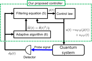
Owing to the work of Liang et al.[21], there is an acceptable uncertainty of the parameter θ\theta that ensures the convergence of the state to the target state. Hence, we only focus on the parameter tuning of M^(t)\hat{M}(t). The adaptive model is then described as follows (Fig. 1).

dρ^(t)=\displaystyle d\hat{\rho}(t)= i[Hω^(u(t)),ρ^(t)]dtM^(t)2[Jz,[Jz,ρ^(t)]]dt\displaystyle\mathrm{i}[H_{\hat{\omega}}(u(t)),\hat{\rho}(t)]_{-}dt-\frac{\hat{M}(t)}{2}[J_{z},[J_{z},\hat{\rho}(t)]_{-}]_{-}dt
+η^M^(t)(Jzρ^(t)+ρ^(t)Jz2Tr[Jzρ^(t)]ρ^(t))\displaystyle+\sqrt{\hat{\eta}\hat{M}(t)}\left(J_{z}\hat{\rho}(t)+\hat{\rho}(t)J_{z}-2\mathrm{Tr}[J_{z}\hat{\rho}(t)]\hat{\rho}(t)\right)
×(dy(t)2η^M^(t)Tr[Jzρ^(t)]dt),\displaystyle\quad\quad\times\left(dy(t)-2\sqrt{\hat{\eta}\hat{M}(t)}\mathrm{Tr}[J_{z}\hat{\rho}(t)]dt\right), (5)

where (ω^,M^(0),η^)(\hat{\omega},\hat{M}(0),\hat{\eta}) are given and M^(t)\hat{M}(t) is calculated by our proposed parameter tuning algorithm below.
Refer to caption
Figure 1: The proposed adaptive controller

III-A Proposed Adaptive Parameter Tuning Method

For convenience, we use θ^(t):=η^M^(t)\hat{\theta}(t):=\sqrt{\hat{\eta}\hat{M}(t)}, x^(t):=Tr[Jzρ^(t)]\hat{x}(t):=\mathrm{Tr}[J_{z}\hat{\rho}(t)], and x(t):=Tr[Jzρ(t)]x(t):=\mathrm{Tr}[J_{z}\rho(t)]. Then, we propose the following parameter tuning algorithm.

dθ^(t)=\displaystyle d\hat{\theta}(t)= f(t){x^(t)2θ^(t)dt+12x^(t)dy(t)},\displaystyle f(t)\left\{-\hat{x}(t)^{2}\hat{\theta}(t)dt+\frac{1}{2}\hat{x}(t)dy(t)\right\}, (6)
f(t):=\displaystyle f(t):= (Kt+1)p,t0,\displaystyle(Kt+1)^{-p},\quad t\geq 0, (7)

where p(0,1]p\in(0,1] and K>0K>0. Note that we update M^(t)\hat{M}(t) as M^(t)=θ^(t)2/η^\hat{M}(t)=\hat{\theta}(t)^{2}/\hat{\eta}. From the filtering theory [25, 26], dy(t)dy(t) can be replaced by dw(t)+2θx(t)dw(t)+2\theta x(t), where w(t)w(t) is a standard Wiener process, and (6) then gives

dθ^(t)=\displaystyle d\hat{\theta}(t)= f(t)x^(t){(θx(t)θ^(t)x^(t))dt+12dw(t)}.\displaystyle f(t)\hat{x}(t)\left\{(\theta x(t)-\hat{\theta}(t)\hat{x}(t))dt+\frac{1}{2}dw(t)\right\}.

If the noise w(t)w(t) is removed, updating θ^(t)\hat{\theta}(t) by Eq. (6) implies the same as instant gradient method of the cost function |θx(t)θ^(t)x^(t)|2|\theta x(t)-\hat{\theta}(t)\hat{x}(t)|^{2} with the weight f(t)f(t). This is a type of Robbins-Monro algorithm for continuous-time problems [27, 28, 29]. Clearly, if x(t)=x^(t)0x(t)=\hat{x}(t)\neq 0 for all t0t\geq 0, then the parameter tuning law is the continuous-time Robbins-Monro algorithm, which is guaranteed to converge to the true parameter. Unfortunately, the assumption x(t)=x^(t)0x(t)=\hat{x}(t)\neq 0 t0\forall t\geq 0 may not hold; therefore, we need to seek the condition when the parameter θ^(t)\hat{\theta}(t) converges to the region described by (4). Note that the true parameter θ\theta cannot be an equilibrium point of the system (6). Thus, the noise ww is unavoidable, so we examine how to choose the parameter (K,p)(K,p) and obtain the accurate estimate asymptotically.

Remark 3

Because each unknown parameter is a positive constant, the adaptive parameter θ^(t)\hat{\theta}(t) must to be positive. However, the solution of (6) is not ensured to be positive, so when θ^(t)\hat{\theta}(t) becomes negative, we replace it with 0 or a small positive number in practical implementations.

III-B Asymptotic Property of the Estimate

Here, we describe that the choice of the parameters pp and KK of (7) is valid from the following proposition. For convenience, we write 𝔼w[]𝔼w[|ρ(0),ρ^(0)]\mathbb{E}_{w}[\bullet]\equiv\mathbb{E}_{w}[\bullet|\rho(0),\hat{\rho}(0)].

Proposition 4

Suppose that a pair of initial states (ρ(0),ρ^(0))(\rho(0),\hat{\rho}(0)) is in some (ρn,ρm)(\rho_{n},\rho_{m}), mJm\neq J, and u(t)=0u(t)=0, and considering (6) with pp\in\mathbb{R} and K>0K>0, the followings hold.

  1. 1.

    For the mean of the θ^(t)\hat{\theta}(t),

    limt𝔼w[θ^(t)]=\displaystyle\lim_{t\to\infty}\mathbb{E}_{w}[\hat{\theta}(t)]= {(depend on θ^(0)),p>1,θJnJm,p(,1].\displaystyle\left\{\begin{array}[]{ll}\mbox{(depend on $\hat{\theta}(0)$)},&p>1,\\ \theta\frac{J-n}{J-m},&p\in(-\infty,1].\end{array}\right.
  2. 2.

    For the variance of the θ^(t)\hat{\theta}(t), V(θ^(t)):=𝔼w[(θ^(t)𝔼w[θ^(t)])2]V(\hat{\theta}(t)):=\mathbb{E}_{w}[(\hat{\theta}(t)-\mathbb{E}_{w}[\hat{\theta}(t)])^{2}],

    lim suptV(θ^(t))\displaystyle\limsup_{t\to\infty}V(\hat{\theta}(t))\leq 18,p>1,\displaystyle\ \frac{1}{8},\quad p>1,
    limtV(θ^(t))=\displaystyle\lim_{t\to\infty}V(\hat{\theta}(t))= {0,p(0,1],18,p=0,,p<0.\displaystyle\left\{\begin{array}[]{ll}0,&p\in(0,1],\\ \frac{1}{8},&p=0,\\ \infty,&p<0.\end{array}\right.
Proof:

Denote the integral of f(t)f(t) by

F(t):=\displaystyle F(t):= 0tf(τ)𝑑τ\displaystyle\int_{0}^{t}f(\tau)d\tau
=\displaystyle= {1K(1p){(Kt+1)1p1},p{1},1Kln(Kt+1),p=1.\displaystyle\left\{\begin{array}[]{ll}\frac{1}{K(1-p)}\{(Kt+1)^{1-p}-1\},&p\in\mathbb{R}\setminus\{1\},\\ \frac{1}{K}\ln(Kt+1),&p=1.\end{array}\right. (10)

We only prove the convergence of V(θ^(t))V(\hat{\theta}(t)). Note that x=Jnx=J-n and x^=Jm\hat{x}=J-m from the assumption. Then, the explicit solution of V(θ^(t))V(\hat{\theta}(t)) is

V(θ^(t))=\displaystyle V(\hat{\theta}(t))= e2x^2F(t)V(θ^(0))\displaystyle e^{-2\hat{x}^{2}F(t)}V(\hat{\theta}(0))
+x^24e2x^2F(t)0te2x^2F(τ)f(τ)2𝑑τ.\displaystyle+\frac{\hat{x}^{2}}{4}e^{-2\hat{x}^{2}F(t)}\int_{0}^{t}e^{2\hat{x}^{2}F(\tau)}f(\tau)^{2}d\tau.

As θ\theta is a deterministic uncertain parameter and M^(0)\hat{M}(0) is given, V(θ^(0))=0V(\hat{\theta}(0))=0. If p=0p=0, it implies that f(t)=1f(t)=1 and therefore, the claim of the theorem trivially holds. The other cases are as follows.

  1. 1.

    If p(0,)p\in(0,\infty), f(t)2f(t)f(t)^{2}\leq f(t) because f(t)[0,1]f(t)\in[0,1] and f(t)f(τ0)f(t)\leq f(\tau_{0}) for all tτ0t\geq\tau_{0}, where τ0>0\tau_{0}>0 is arbitrary chosen. From simple calculation and using the above-mentioned properties,

    0te2x^2F(τ)f(τ)2𝑑τ\displaystyle\int_{0}^{t}e^{2\hat{x}^{2}F(\tau)}f(\tau)^{2}d\tau
    =\displaystyle= 0τ0e2x^2F(τ)f(τ)2𝑑τ+τ0te2x^2F(τ)f(τ)2𝑑τ\displaystyle\int_{0}^{\tau_{0}}e^{2\hat{x}^{2}F(\tau)}f(\tau)^{2}d\tau+\int_{\tau_{0}}^{t}e^{2\hat{x}^{2}F(\tau)}f(\tau)^{2}d\tau
    \displaystyle\leq 0τ0e2x^2F(τ)f(τ)𝑑τ+f(τ0)τ0te2x^2F(τ)f(τ)𝑑τ\displaystyle\int_{0}^{\tau_{0}}e^{2\hat{x}^{2}F(\tau)}f(\tau)d\tau+f(\tau_{0})\int_{\tau_{0}}^{t}e^{2\hat{x}^{2}F(\tau)}f(\tau)d\tau
    =\displaystyle= F(0)F(τ0)e2x^2s𝑑s+f(τ0)F(τ0)F(t)e2x^2s𝑑s\displaystyle\int_{F(0)}^{F(\tau_{0})}e^{2\hat{x}^{2}s}ds+f(\tau_{0})\int_{F(\tau_{0})}^{F(t)}e^{2\hat{x}^{2}s}ds
    =\displaystyle= 12x^2{e2x^2F(τ0)e2x^2F(0)\displaystyle\frac{1}{2\hat{x}^{2}}\Big{\{}e^{2\hat{x}^{2}F(\tau_{0})}-e^{2\hat{x}^{2}F(0)}
    +f(τ0)e2x^2F(t)f(τ0)e2x^2F(τ0)},\displaystyle\quad\quad\quad+f(\tau_{0})e^{2\hat{x}^{2}F(t)}-f(\tau_{0})e^{2\hat{x}^{2}F(\tau_{0})}\Big{\}},

    and therefore,

    V(θ^(t))\displaystyle V(\hat{\theta}(t))\leq f(τ0)8(1e2x^2(F(t)F(τ0))\displaystyle\frac{f(\tau_{0})}{8}(1-e^{-2\hat{x}^{2}(F(t)-F(\tau_{0})})
    +18e2x^2F(t){e2x^2F(τ0)e2x^2F(0)}.\displaystyle+\frac{1}{8}e^{-2\hat{x}^{2}F(t)}\Big{\{}e^{2\hat{x}^{2}F(\tau_{0})}-e^{2\hat{x}^{2}F(0)}\Big{\}}.

    As τ0\tau_{0} can be chosen to be arbitrarily large, the first term of the right-hand side of the above equation can be arbitrarily small. As tt\to\infty, e2x^2F(t)0e^{-2\hat{x}^{2}F(t)}\to 0 for p(0,1]p\in(0,1] and e2x^2F(t)e2x^2/(K(p1))>0e^{-2\hat{x}^{2}F(t)}\to e^{-2\hat{x}^{2}/(K(p-1))}>0 for p>1p>1. Then, the last term of the right-hand side of the equation remains finite and it is less than 1/81/8. Therefore, the claim of the theorem holds for p(0,)p\in(0,\infty).

  2. 2.

    If p(,0)p\in(-\infty,0), f(t)2f(t)f(t)^{2}\geq f(t) because f(t)1f(t)\geq 1 and f(t)f(τ0)f(t)\geq f(\tau_{0}) for all tτ0t\geq\tau_{0}, where τ0>0\tau_{0}>0 is arbitrary chosen. From simple calculation and using the above-mentioned properties,

    0te2x^2F(τ)f(τ)2𝑑τ\displaystyle\int_{0}^{t}e^{2\hat{x}^{2}F(\tau)}f(\tau)^{2}d\tau
    \displaystyle\geq 0τ0e2x^2F(τ)f(τ)𝑑τ+f(τ0)τ0te2x^2F(τ)f(τ)𝑑τ\displaystyle\int_{0}^{\tau_{0}}e^{2\hat{x}^{2}F(\tau)}f(\tau)d\tau+f(\tau_{0})\int_{\tau_{0}}^{t}e^{2\hat{x}^{2}F(\tau)}f(\tau)d\tau
    \displaystyle\geq f(τ0)2x^2{e2x^2F(t)e2x^2F(τ0)}\displaystyle\frac{f(\tau_{0})}{2\hat{x}^{2}}\Big{\{}e^{2\hat{x}^{2}F(t)}-e^{2\hat{x}^{2}F(\tau_{0})}\Big{\}}

    and therefore, for t>τ0t>\tau_{0}

    V(θ^(t))\displaystyle V(\hat{\theta}(t))\geq f(τ0)8(1e2x^2(F(t)F(τ0)))\displaystyle\frac{f(\tau_{0})}{8}\left(1-e^{-2\hat{x}^{2}(F(t)-F(\tau_{0}))}\right)

    holds. The second term of the right-hand side of the above inequality vanishes as tt\to\infty and because f(τ0)f(\tau_{0}) can be arbitrarily large, if τ0\tau_{0} is large, then V(θ^(t))V(\hat{\theta}(t))\to\infty as tt\to\infty.

From Proposition 4, if ρ(t)\rho(t) and ρ^(t)\hat{\rho}(t) are in the same equilibrium state, the parameter θ^(t)\hat{\theta}(t) updated by (6) converges to the true value with probability one. Unfortunately, since the true state ρ(t)\rho(t) is not accessible, we cannot confirm whether ρ(t)\rho(t) and ρ^(t)\hat{\rho}(t) are practically in the same equilibrium state. To avoid being trapped in different equilibrium points before learning the parameter accurately, we employ feedforward control in the following subsection.

Remark 5

A key to prove Proposition 4 is that, f:[0,)[0,1]f:[0,\infty)\to[0,1] is a non-increasing function with limtf(t)=0\lim_{t\to\infty}f(t)=0, while its integral F(t)=0tf(τ)𝑑τF(t)=\int_{0}^{t}f(\tau)d\tau becomes a non-decreasing function with limtF(t)=\lim_{t\to\infty}F(t)=\infty. This is a minor difference from the continuous-time Robbins-Monro algorithms because they require the square integrability of the function f(t)f(t) (e.g., [28, Theorem 1]). Searching for a preferable function for learning θ\theta is beyond the scope of this study, and we only use (7) and do not consider other functions. We established some convergence rate problems in [30], which can be referred for details.

III-C Local Convergence Property

In this subsection, we evaluate our tuning algorithm (6) with the following control input.

u(t)=\displaystyle u(t)= uFB(ρ^(t))+uFF(t),\displaystyle u_{FB}(\hat{\rho}(t))+u_{FF}(t),

where uFF(t)[0,)u_{FF}(t)\in[0,\infty) is a strictly decreasing, bounded continuous function with limtuFF(t)=0\lim_{t\to\infty}u_{FF}(t)=0, and uFBu_{FB} is a stabilizing feedback control law if θ^(t)\hat{\theta}(t) satisfies the condition of Corollary 2 (e.g., of (4.22) or (4.23) in [21].) The role of uFFu_{FF} is to eliminate the ρ^(t)\hat{\rho}(t) from the target state ρn¯\rho_{\bar{n}} before learning the parameter accurately. Then, our proposed method ensures local convergence under certain assumptions. For convenience, we write 𝔼w[]:=𝔼w[|ρ(t0),ρ^(t0)]\mathbb{E}_{w}^{\prime}[\bullet]:=\mathbb{E}_{w}[\bullet|\rho(t_{0}),\hat{\rho}(t_{0})].

Theorem 6

Let t0>0t_{0}>0 satisfy f(t0)<εf(t_{0})<\varepsilon for a given sufficiently small ε>0\varepsilon>0. Considering ρ(t)\rho(t) and ρ^(t)\hat{\rho}(t) are the solutions of (1) and (5) starting from ρ(t0)\rho(t_{0}), ρ^(t0)𝒮()\hat{\rho}(t_{0})\in\mathcal{S}(\mathbb{\mathbb{C}^{N}}), respectively, we choose the feedforward control uFF(t)u_{FF}(t) that satisfies uFF(t)f(t)2u_{FF}(t)\leq f(t)^{2} for all tt0t\geq t_{0} and the feedback control uFBu_{FB} that satisfies 𝔼w[|uFB(ρ^)|]=O(ε2)\mathbb{E}_{w}^{\prime}[|u_{FB}(\hat{\rho})|]=O(\varepsilon^{2}) if ρ^\hat{\rho} satisfies 𝔼w[ρ^ρn¯Tr]<ε\mathbb{E}_{w}^{\prime}[\|\hat{\rho}-\rho_{\bar{n}}\|_{\mathrm{Tr}}]<\varepsilon. Let θ^(t)\hat{\theta}(t) be the solution of the parameter tuning algorithm (6) with p(0.5,1]p\in(0.5,1] and K>0K>0 and its initial value θ^(t0)\hat{\theta}(t_{0}) satisfy |1θ^(t0)/θ|<ε|1-\hat{\theta}(t_{0})/\theta|<\varepsilon. Suppose that max{𝔼w[ρ(t)ρn¯Tr],𝔼w[ρ^(t)ρn¯Tr]}<ε\max\{\mathbb{E}_{w}^{\prime}[\|\rho(t)-\rho_{\bar{n}}\|_{\mathrm{Tr}}],\mathbb{E}_{w}^{\prime}[\|\hat{\rho}(t)-\rho_{\bar{n}}\|_{\mathrm{Tr}}]\}<\varepsilon and max{𝔼w[ρ(t)ρn¯Tr2],𝔼w[ρ^(t)ρn¯Tr2]}<ε2\max\{\mathbb{E}_{w}^{\prime}[\|\rho(t)-\rho_{\bar{n}}\|_{\mathrm{Tr}}^{2}],\mathbb{E}_{w}^{\prime}[\|\hat{\rho}(t)-\rho_{\bar{n}}\|_{\mathrm{Tr}}^{2}]\}<\varepsilon^{2} for all tt0t\geq t_{0}. Besides, assume that the following inequality holds for almost all tt0t\geq t_{0}

Δ(ρ(t),ρ^(t),θ^(t))0 a.s.,\displaystyle\Delta(\rho(t),\hat{\rho}(t),\hat{\theta}(t))\geq 0\quad\mbox{ a.s.,} (11)

and the equality holds iff Vρ(t)(Jz)=Vρ^(t)(Jz)=0V_{\rho(t)}(J_{z})=V_{\hat{\rho}(t)}(J_{z})=0, where

Δ(ρ,ρ^,θ^)\displaystyle\Delta(\rho,\hat{\rho},\hat{\theta})
:=\displaystyle:= (3Vρ(Jz)2+2Vρ(Jz)Vρ^(Jz)+3Vρ^(Jz)2)\displaystyle\left(3V_{\rho}(J_{z})^{2}+2V_{\rho}(J_{z})V_{\hat{\rho}}(J_{z})+3V_{\hat{\rho}}(J_{z})^{2}\right)
2Vρ^(Jz)(Tr[Jz(ρρ^)]+Tr[Jzρ^](1θ^θ)),\displaystyle-2V_{\hat{\rho}}(J_{z})\left(\mathrm{Tr}[J_{z}(\rho-\hat{\rho})]+\mathrm{Tr}[J_{z}\hat{\rho}]\left(1-\frac{\hat{\theta}}{\theta}\right)\right),

Vρ(Jz):=Tr[Jz2ρ]Tr[Jzρ]2V_{\rho}(J_{z}):=\mathrm{Tr}[J_{z}^{2}\rho]-\mathrm{Tr}[J_{z}\rho]^{2}. Then, for n¯J\bar{n}\neq J,

limt(ρ(t),ρ^(t))=(ρn¯,ρn¯) and limtθ^(t)=θa.s.\displaystyle\lim_{t\to\infty}(\rho(t),\hat{\rho}(t))=(\rho_{\bar{n}},\rho_{\bar{n}})\mbox{ and }\lim_{t\to\infty}\hat{\theta}(t)=\theta\ \mbox{a.s.}
Proof:

See Appendix.

Some readers may think the assumptions of Theorem 6 are too strong to be valid in practice; however, several numerical experiments support that they may hold in many cases, one of which is demonstrated in the following section.

IV NUMERICAL EXPERIMENTS

In this section, we examine the proposed method numerically. The dimension of the quantum system is N=5N=5, and the Euler-Maruyama method is used with 0.010.01 time step width. We use the true parameters as (ω,M,η)=(0.5,1,0.9)(\omega,M,\eta)=(0.5,1,0.9) and the initial parameters of the adaptive system as (ω^,M^(0),η^)=(1,25,1)(\hat{\omega},\hat{M}(0),\hat{\eta})=(1,25,1), for which the system cannot be stabilized by merely using the feedback control in [21]. The true initial state ρ(0)\rho(0) is randomly generated for each realization and the initial adaptive state is fixed to ρ^(0)=1NI\hat{\rho}(0)=\frac{1}{N}I. The target state ρn¯\rho_{\bar{n}} is set as n¯=0\bar{n}=0. We set the control inputs as follows.

uFF(t):=f(t)2,uFB(ρ^):=\displaystyle u_{FF}(t):=f(t)^{2},\quad u_{FB}(\hat{\rho}):= 4(1Tr[ρ^ρn¯])2.\displaystyle 4(1-\mathrm{Tr}[\hat{\rho}\rho_{\bar{n}}])^{2}.

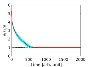
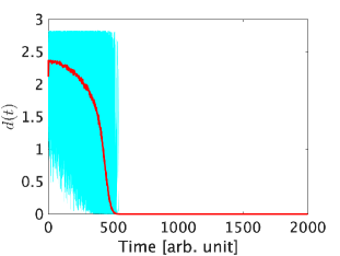
The parameters of (7) are chosen as (K,p)=(20,0.6)(K,p)=(20,0.6), and then the simulation is run with 1000 realizations. The results are shown in Figs. 2 and 3. Fig. 2 represents the trajectories of the ratio θ^(t)/θ\hat{\theta}(t)/\theta and Fig. 3 represents the distance d(t)=dB((ρ(t),ρ^(t)),(ρn¯,ρn¯))d(t)=d_{B}((\rho(t),\hat{\rho}(t)),(\rho_{\bar{n}},\rho_{\bar{n}})) [21],

dB((ρ,ρ^),(ρn,ρm))\displaystyle d_{B}((\rho,\hat{\rho}),(\rho_{n},\rho_{m}))
=\displaystyle= 22Tr[ρρn]+22Tr[ρ^ρm].\displaystyle\sqrt{2-2\sqrt{\mathrm{Tr}[\rho\rho_{n}]}}+\sqrt{2-2\sqrt{\mathrm{Tr}[\hat{\rho}\rho_{m}]}}.

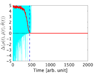
We also evaluate whether the inequality (11) holds in Fig. 4. From the figures, all sample trajectories of θ^(t)\hat{\theta}(t) and (ρ(t),ρ^(t))(\rho(t),\hat{\rho}(t)) appear to converge to θ\theta and the target state ρ0\rho_{0}, respectively. The inequality (11) sometimes does not hold at the beginning of the simulations, but all sample trajectories satisfy it after t=450t=450, shown by the blue dashed line in Fig. 4, until the states converge to the target states. Moreover, even though our proposed method does not ensure satisfying the condition (3) at all times after a certain point, we confirmed that all sample trajectories of the θ^(t)/θ\hat{\theta}(t)/\theta ratio satisfy the condition of Corollary 2, i.e., θ^(t)/θ(1+α0,1+β0)(0.889,1.11)\hat{\theta}(t)/\theta\in(1+\alpha_{0},1+\beta_{0})\simeq(0.889,1.11), after t=666t=666. This result implies that the proposed method ensures that all sample trajectories are in the neighborhood of the true value with a significantly high probability. Although we confirmed that (K,p)=(20,0.3)(K,p)=(20,0.3), which does not satisfy the condition of Theorem 6, also works well, but the result is omitted due to the page limitation.
Refer to caption
Figure 2: The trajectories of the ratio θ^(t)/θ\hat{\theta}(t)/\theta with parameters (K,p)=(20,0.6)(K,p)=(20,0.6). The solid red line represents the average trajectory over 1000 samples and the light blue lines represent 1000 sample realizations.
Refer to caption
Figure 3: The trajectories of d(t)d(t) with parameters (K,p)=(K,p)=(20, 0.6). The solid red line represents the average trajectory over 1000 samples and the light blue lines represent 1000 sample realizations.
Refer to caption
Figure 4: The trajectories of Δ(ρ(t),ρ^(t),θ^(t))\Delta(\rho(t),\hat{\rho}(t),\hat{\theta}(t)) with parameters (K,p)=(K,p)=(20, 0.6). The solid red line represents the average trajectory over 1000 samples and the light blue lines represent 1000 sample realizations. The blue dashed line represents the time 450.

V CONCLUSION AND FUTURE WORK

In this paper, we proposed an adaptive parameter tuning algorithm for robust stabilizing control of quantum angular momentum systems. The asymptotic property of the estimate and local convergence of the states were evaluated analytically, and numerical experiments show that the proposed method works well for systems with large parametric uncertainty.

The relaxation of Theorem 6’s assumptions and the global convergence property are interesting works for future.

ACKNOWLEDGMENTS

The authors gratefully acknowledge the helpful comments and suggestions of the anonymous reviewers.

References

  • [1] R. van Handel, J. K. Stockton, and H. Mabuchi, “Feedback control of quantum state reduction,” IEEE Transactions on Automatic Control, vol. 50, no. 6, pp. 768–780, 2005.
  • [2] M. Mirrahimi and R. van Handel, “Stabilizing Feedback Controls for quantum systems,” SIAM Journal on Control and Optimization, vol. 46, no. 2, pp. 445–467, 2007.
  • [3] K. Tsumura, “Global stabilization of n-dimensional quantum spin systems via continuous feedback,” in Proceedings of 2007 American Control Conference.   IEEE, 2007, pp. 2129–2134.
  • [4] A. Sarlette, Z. Leghtas, M. Brune, J. M. Raimond, and P. Rouchon, “Stabilization of nonclassical states of one- and two-mode radiation fields by reservoir engineering,” Physical Review A, vol. 86, p. 012114, Jul 2012.
  • [5] F. Ticozzi, R. Lucchese, P. Cappellaro, and L. Viola, “Hamiltonian Control of Quantum Dynamical Semigroups: Stabilization and Convergence Speed,” IEEE Transaction on Automatic Control, vol. 57, no. 8, pp. 1931–1944, 2012.
  • [6] F. Ticozzi, K. Nishio, and C. Altafini, “Stabilization of Stochastic Quantum Dynamics via Open and Closed Loop Control,” IEEE Transaction on Automatic Control, vol. 58, pp. 74–85, 2013.
  • [7] P. Scaramuzza and F. Ticozzi, “Switching quantum dynamics for fast stabilization,” Physical Review A, vol. 91, p. 062314, Jun 2015.
  • [8] F. Ticozzi, L. Zuccato, P. D. Johnson, and L. Viola, “Alternating projections methods for discrete-time stabilization of quantum states,” IEEE Transactions on Automatic Control, vol. 63, no. 3, pp. 819–826, 2017.
  • [9] W. Liang, N. H. Amini, and P. Mason, “On exponential stabilization of NN-level quantum angular momentum systems,” SIAM Journal on Control and Optimization, vol. 57, no. 6, pp. 3939–3960, 2019.
  • [10] G. Cardona, A. Sarlette, and P. Rouchon, “Exponential stabilization of quantum systems under continuous non-demolition measurements,” Automatica, vol. 112, p. 108719, 2020.
  • [11] J. Wen, Y. Shi, J. Jia, and J. Zeng, “Exponential stabilization of two-level quantum systems based on continuous noise-assisted feedback,” Results in Physics, vol. 22, p. 103929, 2021.
  • [12] K. Zhou, J. C. Doyle, and K. Glover, Robust and Optimal Control.   Prentice Hall Upper Saddle River, NJ, 1996.
  • [13] I. R. Petersen, V. A. Ugrinovskii, and A. V. Savkin, Robust Control Design using HH^{\infty} Methods.   Springer Verlag, 2000.
  • [14] K. S. Narendra and A. M. Annaswamy, Stable Adaptive Systems.   Prentice-Hall, Inc. Upper Saddle River, NJ, USA, 1989.
  • [15] M. Krstic, P. V. Kokotovic, and I. Kanellakopoulos, Nonlinear and Adaptive Control Design.   John Wiley & Sons, Inc., 1995.
  • [16] M. R. James, “Risk-sensitive optimal control of quantum systems,” Physical Review A, vol. 69, no. 3, p. 032108, 2004.
  • [17] ——, “A quantum Langevin formulation of risk-sensitive optimal control,” Journal of Optics B: Quantum and Semiclassical Optics, vol. 7, p. S198, 2005.
  • [18] D. Dong, C. Chen, B. Qi, I. R. Petersen, and F. Nori, “Robust manipulation of superconducting qubits in the presence of fluctuations,” Scientific Reports, vol. 5, p. 7873, 2015.
  • [19] I. G. Vladimirov, I. R. Petersen, and M. R. James, “Risk-sensitive performance criteria and robustness of quantum systems with a relative entropy description of state uncertainty,” in 23rd International Symposium on Mathematical Theory of Networks and Systems, Hong Kong, Jul. 2018, pp. 482–488.
  • [20] M. R. James, H. I. Nurdin, and I. R. Petersen, “HH^{\infty} Control of Linear Quantum Stochastic Systems,” IEEE Transactions on Automatic Control, vol. 53, no. 8, pp. 1787–1803, 2008.
  • [21] W. Liang, N. H. Amini, and P. Mason, “Robust Feedback Stabilization of NN-Level Quantum Spin Systems,” SIAM Journal on Control and Optimization, vol. 59, no. 1, pp. 669–692, jan 2021.
  • [22] S. Bonnabel, M. Mirrahimi, and P. Rouchon, “Observer-based Hamiltonian identification for quantum systems,” Automatica, vol. 45, no. 5, pp. 1144–1155, 2009.
  • [23] Z. Leghtas, M. Mirrahimi, and P. Rouchon, “Back and forth nudging for quantum state estimation by continuous weak measurement,” in Proceedings of the 2011 American Control Conference.   IEEE, 2011.
  • [24] R. S. Gupta and M. J. Biercuk, “Adaptive filtering of projective quantum measurements using discrete stochastic methods,” Physical Review A, vol. 104, p. 012412, 2021.
  • [25] L. Bouten, R. van Handel, and M. R. James, “An Introduction to Quantum Filtering,” SIAM Journal on Control and Optimization, vol. 46, no. 6, pp. 2199–2241, 2007.
  • [26] A. Bain and D. Crişan, Fundamentals of Stochastic Filtering, ser. Stochastic Modelling and Applied Probability.   Springer Verlag, 2009, vol. 60.
  • [27] H. Robbins and S. Monro, “A Stochastic Approximation Method,” The Annals of Mathematical Statistics, vol. 22, no. 3, pp. 400–407, 1951.
  • [28] H.-F. Chen, “Continuous-time stochastic approximation: convergence and asymptotic efficiency,” Stochastics and Stochastic Reports, vol. 51, no. 3-4, pp. 217–239, 1994.
  • [29] H. Kushner, “Stochastic approximation: a survey,” Wiley Interdisciplinary Reviews: Computational Statistics, vol. 2, no. 1, pp. 87–96, 2010.
  • [30] S. Enami and K. Ohki, “Convergence analysis of adaptive tuning parameter for robust stabilizing control of NN -level quantum systems,” in Proceedings of 60th Annual Conference of the Society of Instrument and Control Engineers of Japan, 2021.
  • [31] X. Mao, “Stochastic versions of the LaSalle theorem,” Journal of Differential Equations, vol. 153, no. 1, pp. 175–195, 1999.
  • [32] H. J. Kushner, Stochastic Stability and Control, Academic Press, 1967.

Proof of Theorem 6

To prove Theorem 6, we evaluate G(ρ(t),ρ^(t),θ^(t)):=Cx(t)+Cθ(t)+Vρ(t)(Jz)+Vρ^(t)(Jz)G(\rho(t),\hat{\rho}(t),\hat{\theta}(t)):=C_{x}(t)+C_{\theta}(t)+V_{\rho(t)}(J_{z})+V_{\hat{\rho}(t)}(J_{z}), where Cθ(t):=|1θ^(t)θ|2C_{\theta}(t):=\left|1-\frac{\hat{\theta}(t)}{\theta}\right|^{2}, and Cx(t):=|x(t)x^(t)|2C_{x}(t):=|x(t)-\hat{x}(t)|^{2}. Our proof mainly follows the argument of the proof of Theorem 2.1 in [31].

First, we evaluate Vρ^(t)(Jz)V_{\hat{\rho}(t)}(J_{z}) and Vρ(t)(Jz)V_{\rho(t)}(J_{z}).

Lemma 7

If 𝔼w[ρ^(t)ρn¯Tr]<ε\mathbb{E}_{w}^{\prime}[\|\hat{\rho}(t)-\rho_{\bar{n}}\|_{\mathrm{Tr}}]<\varepsilon holds for some small ε>0\varepsilon>0, then

Vρ^(t)(Jz)=εα^(t)+ε2Tr[(ρ^(t)ρn¯)Jz]2,\displaystyle V_{\hat{\rho}(t)}(J_{z})=\varepsilon\hat{\alpha}(t)+\varepsilon^{2}\mathrm{Tr}[(\hat{\rho}(t)-\rho_{\bar{n}})J_{z}]^{2},

where α^(t):=Tr[(ρ^(t)ρn¯)(Jz(Jn¯)In)2]\hat{\alpha}(t):=\mathrm{Tr}[(\hat{\rho}(t)-\rho_{\bar{n}})(J_{z}-(J-\bar{n})I_{n})^{2}] is a nonnegative number and α(t)=0\alpha(t)=0 iff ρ^(t)=ρn¯\hat{\rho}(t)=\rho_{\bar{n}}.

Proof:

If 𝔼w[ρ^(t)ρTr]<ε\mathbb{E}_{w}^{\prime}[\|\hat{\rho}(t)-\rho\|_{\mathrm{Tr}}]<\varepsilon holds for some small ε>0\varepsilon>0, there exists X(t)=X(t)N×NX(t)=X(t)^{\ast}\in\mathbb{C}^{N\times N} that satisfies ρ^(t)=ρ+εX(t)\hat{\rho}(t)=\rho+\varepsilon X(t) and 𝔼w[X(t)Tr]<1\mathbb{E}_{w}^{\prime}[\|X(t)\|_{\mathrm{Tr}}]<1. This implies that if 𝔼w[ρ^(t)ρn¯Tr]<ε\mathbb{E}_{w}^{\prime}[\|\hat{\rho}(t)-\rho_{\bar{n}}\|_{\mathrm{Tr}}]<\varepsilon holds for a small ε>0\varepsilon>0, then

Vρ^(t)(Jz)=εTr[X(t)(Jz(Jn¯)In)2]=α^(t)+ε2Tr[X(t)Jz]2\displaystyle V_{\hat{\rho}(t)}(J_{z})=\varepsilon\underbrace{\mathrm{Tr}[X(t)(J_{z}-(J-\bar{n})I_{n})^{2}]}_{=\hat{\alpha}(t)}+\varepsilon^{2}\mathrm{Tr}[X(t)J_{z}]^{2}

holds. Since ρn¯+εX(t)𝒮(N)\rho_{\bar{n}}+\varepsilon X(t)\in\mathcal{S}(\mathbb{C}^{N}), the (n¯+1)(\bar{n}+1)-th diagonal element of X(t)X(t) needs to be nonpositive and the other diagonal elements are nonnegative, and Tr[X(t)]=0\mathrm{Tr}[X(t)]=0. The (n¯+1)(\bar{n}+1)-th diagonal element of (Jz(Jn¯)In)2(J_{z}-(J-\bar{n})I_{n})^{2} becomes 0, so α^(t)\hat{\alpha}(t) is nonnegative and α^(t)=0\hat{\alpha}(t)=0 iff ρ^(t)=ρn¯\hat{\rho}(t)=\rho_{\bar{n}}.

Therefore, 𝔼w[Vρ^(t)(Jz)]=O(ε)\mathbb{E}_{w}^{\prime}[V_{\hat{\rho}(t)}(J_{z})]=O(\varepsilon). Similar argument gives 𝔼w[Vρ^(t)(Jz)2]=O(ε2)\mathbb{E}_{w}^{\prime}[V_{\hat{\rho}(t)}(J_{z})^{2}]=O(\varepsilon^{2}) and 𝔼w[Vρ(t)(Jz)]=O(ε)\mathbb{E}_{w}^{\prime}[V_{\rho(t)}(J_{z})]=O(\varepsilon) from the assumptions. Note that dy(t)dy(t) in (5) can be replaced by θx(t)dt+dw(t)\theta x(t)dt+dw(t). Let \mathcal{L} be the infinitesimal generator [32]. Using the classical Ito calculus, the infinitesimal generators of Vρ(t)(Jz)V_{\rho(t)}(J_{z}) and Vρ^(t)(Jz)V_{\hat{\rho}(t)}(J_{z}) are as follows.

Vρ(t)(Jz)=\displaystyle\mathcal{L}V_{\rho(t)}(J_{z})= 4θ2Vρ(t)(Jz)2iu(t)Tr[Jy[Jz,ρ(t)]],\displaystyle-4\theta^{2}V_{\rho(t)}(J_{z})^{2}-\mathrm{i}u(t)\mathrm{Tr}[J_{y}[J_{z},\rho(t)]_{-}],
Vρ^(t)(Jz)\displaystyle\mathcal{L}V_{\hat{\rho}(t)}(J_{z})\leq 4θ2Vρ^(t)(Jz)2iu(t)Tr[Jy[Jz,ρ^(t)]]\displaystyle-4\theta^{2}V_{\hat{\rho}(t)}(J_{z})^{2}-\mathrm{i}u(t)\mathrm{Tr}[J_{y}[J_{z},\hat{\rho}(t)]_{-}]
+2θ2Vρ^(t)(Jz)(x(t)x^(t))\displaystyle+2\theta^{2}V_{\hat{\rho}(t)}(J_{z})(x(t)-\hat{x}(t))
+2θx^(t)Vρ^(t)(Jz)(θθ^(t))\displaystyle+2\theta\hat{x}(t)V_{\hat{\rho}(t)}(J_{z})(\theta-\hat{\theta}(t))
+4(θ2θ^(t)2)Vρ^(t)(Jz)2\displaystyle+4(\theta^{2}-\hat{\theta}(t)^{2})V_{\hat{\rho}(t)}(J_{z})^{2}
+2(θ^(t)θ)Vρ^(t)(Jz)(θx(t)θ^(t)x^(t)).\displaystyle+2(\hat{\theta}(t)-\theta)V_{\hat{\rho}(t)}(J_{z})(\theta x(t)-\hat{\theta}(t)\hat{x}(t)).

Since 𝔼w[Vρ(t)(Jz)2]=O(ε2)\mathbb{E}_{w}^{\prime}[V_{\rho(t)}(J_{z})^{2}]=O(\varepsilon^{2}), 𝔼w[[ρ(t),Jz]]=O(ε)\mathbb{E}_{w}^{\prime}[[\rho(t),J_{z}]_{-}]=O(\varepsilon), 𝔼w[[ρ^(t),Jz]]=O(ε)\mathbb{E}_{w}^{\prime}[[\hat{\rho}(t),J_{z}]_{-}]=O(\varepsilon), 𝔼w[uFB(ρ^(t))]=O(ε2)\mathbb{E}_{w}^{\prime}[u_{FB}(\hat{\rho}(t))]=O(\varepsilon^{2}), and uFF(t)=O(f(t)2)u_{FF}(t)=O(f(t)^{2}),

𝔼w[(Vρ(t)(Jz)+Vρ^(t)(Jz))]\displaystyle\mathbb{E}_{w}^{\prime}[\mathcal{L}(V_{\rho(t)}(J_{z})+V_{\hat{\rho}(t)}(J_{z}))]
=\displaystyle= 𝔼w[4θ2(Vρ(t)(Jz)2+Vρ^(t)(Jz)2)+σ1uFF(t)\displaystyle\mathbb{E}_{w}^{\prime}\Bigg{[}-4\theta^{2}(V_{\rho(t)}(J_{z})^{2}+V_{\hat{\rho}(t)}(J_{z})^{2})+\sigma_{1}u_{FF}(t)
+2θ2Vρ^(t)(Jz)((x(t)x^(t))+x^(t)(1θ^(t)θ))]\displaystyle+2\theta^{2}V_{\hat{\rho}(t)}(J_{z})\left((x(t)-\hat{x}(t))+\hat{x}(t)\left(1-\frac{\hat{\theta}(t)}{\theta}\right)\right)\Bigg{]}
+O(ε3)+O(εCθ(t))+O(ε2Cθ(t)),\displaystyle+O(\varepsilon^{3})+O(\varepsilon C_{\theta}(t))+O\left(\varepsilon^{2}\sqrt{C_{\theta}(t)}\right), (12)

where σ1:=maxρ𝒮(N)|Tr[Jy[Jz,ρ]]|\sigma_{1}:=\max_{\rho\in\mathcal{S}(\mathbb{C}^{N})}|\mathrm{Tr}[J_{y}[J_{z},\rho]_{-}]|.

Next, we calculate the infinitesimal generator of Cx(t)C_{x}(t) and Cθ(t)C_{\theta}(t). From simple calculation,

Cx(t)\displaystyle\mathcal{L}C_{x}(t)
\displaystyle\leq 2|uFB(ρ^(t))||Tr[Jy[ρ(t)ρ^(t),Jz]]|Cx(t)\displaystyle 2|u_{FB}(\hat{\rho}(t))|\left|\mathrm{Tr}[J_{y}[\rho(t)-\hat{\rho}(t),J_{z}]_{-}]\right|\sqrt{C_{x}(t)}
+8Jσ1uFF(t)+4θ^(t)θVρ^(t)(Jz)\displaystyle+8J\sigma_{1}u_{FF}(t)+4\hat{\theta}(t)\theta V_{\hat{\rho}(t)}(J_{z})
×{Cx(t)+|x^(t)|Cθ(t)Cx(t)}\displaystyle\quad\times\Bigg{\{}-C_{x}(t)+|\hat{x}(t)|\sqrt{C_{\theta}(t)}\sqrt{C_{x}(t)}\Bigg{\}}
+(θVρ(t)(Jz)θ^(t)Vρ^(t)(Jz))2.\displaystyle+\left(\theta V_{\rho(t)}(J_{z})-\hat{\theta}(t)V_{\hat{\rho}(t)}(J_{z})\right)^{2}.

From the definition of Cθ(t)C_{\theta}(t),

Cθ(t)\displaystyle\mathcal{L}C_{\theta}(t)\leq 2f(t){x^(t)2Cθ(t)+|x^(t)|Cθ(t)Cx(t)\displaystyle 2f(t)\Bigg{\{}-\hat{x}(t)^{2}C_{\theta}(t)+|\hat{x}(t)|\sqrt{C_{\theta}(t)}\sqrt{C_{x}(t)}
+x^(t)2f(t)8θ2}.\displaystyle\hskip 56.9055pt+\frac{\hat{x}(t)^{2}f(t)}{8\theta^{2}}\Bigg{\}}.

Since the expectation of the right-hand side of the above inequality is at most O(ε2)O(\varepsilon^{2}) for small tt0>0t-t_{0}>0, 𝔼w[Cθ(t)]Cθ(t0)=t0t𝔼w[Cθ(τ)]𝑑τ(tt0)×O(ε2)\mathbb{E}_{w}^{\prime}[C_{\theta}(t)]-C_{\theta}(t_{0})=\int_{t_{0}}^{t}\mathbb{E}_{w}^{\prime}[\mathcal{L}C_{\theta}(\tau)]d\tau\leq(t-t_{0})\times O(\varepsilon^{2}), where the Dynkin’s formula [32] is used. Let a(t):=4θ^(t)θVρ^(t)(Jz)a(t):=4\hat{\theta}(t)\theta V_{\hat{\rho}(t)}(J_{z}) and b(t):=2f(t)b(t):=2f(t). Note that a(t)=0a(t)=0 iff Vρ^(t)(Jz)=0V_{\hat{\rho}(t)}(J_{z})=0. Then,

𝔼w[(Cx(t)+Cθ(t))]\displaystyle\mathbb{E}_{w}^{\prime}[\mathcal{L}(C_{x}(t)+C_{\theta}(t))]
\displaystyle\leq 𝔼w[2|uFB(ρ^(t))||Tr[Jy[ρ(t)ρ^(t),Jz]]|Cx(t)\displaystyle\mathbb{E}_{w}^{\prime}\Bigg{[}2|u_{FB}(\hat{\rho}(t))|\left|\mathrm{Tr}[J_{y}[\rho(t)-\hat{\rho}(t),J_{z}]_{-}]\right|\sqrt{C_{x}(t)}
+8Jσ1uFF(t)\displaystyle\quad\quad+8J\sigma_{1}u_{FF}(t)
a(t)Cx(t)b(t)x^(t)2Cθ(t)\displaystyle\quad\quad-a(t)C_{x}(t)-b(t)\hat{x}(t)^{2}C_{\theta}(t)
+(a(t)+b(t))|x^(t)|Cx(t)Cθ(t)\displaystyle\quad\quad+(a(t)+b(t))|\hat{x}(t)|\sqrt{C_{x}(t)C_{\theta}(t)}
+(θVρ(t)(Jz)θ^(t)Vρ^(t)(Jz))2+J2b(t)216θ2]\displaystyle\quad\quad+\left(\theta V_{\rho(t)}(J_{z})-\hat{\theta}(t)V_{\hat{\rho}(t)}(J_{z})\right)^{2}+\frac{J^{2}b(t)^{2}}{16\theta^{2}}\Bigg{]}
=\displaystyle= 𝔼w[θ2(Vρ(t)(Jz)Vρ^(t)(Jz))2O(ε2)\displaystyle\mathbb{E}_{w}^{\prime}\Bigg{[}\underbrace{\theta^{2}\left(V_{\rho(t)}(J_{z})-V_{\hat{\rho}(t)}(J_{z})\right)^{2}}_{O(\varepsilon^{2})}
+J2b(t)216θ2+8Jσ1uFF(t)O(f(t)2)\displaystyle\quad\quad+\underbrace{\frac{J^{2}b(t)^{2}}{16\theta^{2}}+8J\sigma_{1}u_{FF}(t)}_{O(f(t)^{2})}
(a(t)Cx(t)=O(ε3)+b(t)|Jn¯|2Cθ(t)=O(f(t)Cθ(t)))+O(ε4)].\displaystyle\quad\quad-\big{(}\underbrace{a(t)C_{x}(t)}_{=O(\varepsilon^{3})}+\underbrace{b(t)|J-\bar{n}|^{2}C_{\theta}(t)}_{=O(f(t)C_{\theta}(t))}\big{)}+O(\varepsilon^{4})\Bigg{]}. (13)

Note that

𝔼w[|uFB(ρ^(t))||Tr[Jy[ρ(t)ρ^(t),Jz]]|Cx(t)]=O(ε4).\mathbb{E}_{w}^{\prime}[|u_{FB}(\hat{\rho}(t))|\left|\mathrm{Tr}[J_{y}[\rho(t)-\hat{\rho}(t),J_{z}]_{-}]\right|\sqrt{C_{x}(t)}]=O(\varepsilon^{4}).

From (12) and (13),

𝔼w[G(ρ(t),ρ^(t),θ^(t))]\displaystyle\mathbb{E}_{w}^{\prime}\left[\mathcal{L}G(\rho(t),\hat{\rho}(t),\hat{\theta}(t))\right]
\displaystyle\leq 𝔼w[θ2(Vρ(t)(Jz)Vρ^(t)(Jz))2+J2b(t)216θ2\displaystyle\mathbb{E}_{w}^{\prime}\Bigg{[}\theta^{2}\left(V_{\rho(t)}(J_{z})-V_{\hat{\rho}(t)}(J_{z})\right)^{2}+\frac{J^{2}b(t)^{2}}{16\theta^{2}}
+(1+8J)σ1uFF(t)\displaystyle\quad\quad+(1+8J)\sigma_{1}u_{FF}(t)
4θ2(Vρ(t)(Jz)2+Vρ^(t)(Jz)2)\displaystyle\quad\quad-4\theta^{2}\left(V_{\rho(t)}(J_{z})^{2}+V_{\hat{\rho}(t)}(J_{z})^{2}\right)
+2θ2Vρ^(t)(Jz)\displaystyle\quad\quad+2\theta^{2}V_{\hat{\rho}(t)}(J_{z})
×((x(t)x^(t))+x^(t)(1θ^(t)θ))\displaystyle\quad\quad\quad\times\left((x(t)-\hat{x}(t))+\hat{x}(t)\left(1-\frac{\hat{\theta}(t)}{\theta}\right)\right)
b(t)|Jn¯|2Cθ(t)+O(ε3)]\displaystyle\quad\quad-b(t)|J-\bar{n}|^{2}C_{\theta}(t)+O(\varepsilon^{3})\Bigg{]}
=\displaystyle= 𝔼w[Δ(ρ(t),ρ^(t),θ^(t))+b(t)|Jn¯|2Cθ(t)]\displaystyle-\mathbb{E}_{w}^{\prime}\left[\Delta(\rho(t),\hat{\rho}(t),\hat{\theta}(t))+b(t)|J-\bar{n}|^{2}C_{\theta}(t)\right]
+γ(t)+O(ε3),\displaystyle+\gamma(t)+O(\varepsilon^{3}),

where γ(t):=J2b(t)216θ2+(1+8J)σ1uFF(t)\gamma(t):=\frac{J^{2}b(t)^{2}}{16\theta^{2}}+(1+8J)\sigma_{1}u_{FF}(t). As p(0.5,1]p\in(0.5,1], b(t)2=4f(t)2b(t)^{2}=4f(t)^{2} and uFF(t)u_{FF}(t) are integrable, i.e., γ(t)\gamma(t) is integrable.

Together with the assumption (11), 𝔼w[Cθ(t)]O(ε2)\mathbb{E}_{w}^{\prime}[C_{\theta}(t)]\leq O(\varepsilon^{2}) for all tt0t\geq t_{0} and using Dynkin’s formula [32],

𝔼w[G(ρ(),ρ^(),θ^())]G(ρ(t0),ρ^(t0),θ^(t0))\displaystyle\mathbb{E}_{w}^{\prime}\left[G(\rho(\infty),\hat{\rho}(\infty),\hat{\theta}(\infty))\right]-G(\rho(t_{0}),\hat{\rho}(t_{0}),\hat{\theta}(t_{0}))
+t0𝔼w[Δ(ρ(τ),ρ^(τ),θ^(τ))]𝑑τ\displaystyle+\int_{t_{0}}^{\infty}\mathbb{E}_{w}^{\prime}[\Delta(\rho(\tau),\hat{\rho}(\tau),\hat{\theta}(\tau))]d\tau
+|Jn¯|2t0b(τ)𝔼w[Cθ(τ)]𝑑τ+t0𝔼w[O(ε3)]𝑑τ\displaystyle+|J-\bar{n}|^{2}\int_{t_{0}}^{\infty}b(\tau)\mathbb{E}_{w}^{\prime}[C_{\theta}(\tau)]d\tau+\int_{t_{0}}^{\infty}\mathbb{E}_{w}^{\prime}[O(\varepsilon^{3})]d\tau
\displaystyle\leq t0γ(τ)𝑑τ<\displaystyle\int_{t_{0}}^{\infty}\gamma(\tau)d\tau<\infty

holds. Note that the integrand of the last term of the left-hand side of the first inequality 𝔼w[O(ε3)]\mathbb{E}_{w}^{\prime}[O(\varepsilon^{3})] converges to zero faster than the other terms. The other terms of the left-hand side are positive and need to be finite. Hence, limtΔ(ρ(t),ρ^(t),θ^(t))=0\lim_{t\to\infty}\Delta(\rho(t),\hat{\rho}(t),\hat{\theta}(t))=0 a.s. Since x(t)x(t) or x^(t)\hat{x}(t) fluctuates randomly if ρ(t)0\rho(t)\neq 0 or ρ^(t)0\hat{\rho}(t)\neq 0, limtΔ(ρ(t),ρ^(t),θ^(t))=0\lim_{t\to\infty}\Delta(\rho(t),\hat{\rho}(t),\hat{\theta}(t))=0 implies that Vρ(t)(Jz)V_{\rho(t)}(J_{z}) and Vρ^(t)(Jz)V_{\hat{\rho}(t)}(J_{z}) converge to the origin. From the assumption that ρ(t)\rho(t) and ρ^(t)\hat{\rho}(t) stay in the neighborhood of ρn¯\rho_{\bar{n}}, the convergence of Vρ(t)(Jz)V_{\rho(t)}(J_{z}) and Vρ^(t)(Jz)V_{\hat{\rho}(t)}(J_{z}) implies (ρ(t),ρ^(t))(\rho(t),\hat{\rho}(t)) converges to (ρn¯,ρn¯)(\rho_{\bar{n}},\rho_{\bar{n}}). Furthermore, since b(t)b(t) is not integrable and, although we skip the proof, θ^(t)\hat{\theta}(t) is continuous in tt, limtCθ(t)=0\lim_{t\to\infty}C_{\theta}(t)=0 a.s. Therefore, limtθ^(t)=θ\lim_{t\to\infty}\hat{\theta}(t)=\theta a.s.