Samrudhdhi B. [email protected]
\addauthorJames J. [email protected]
\addinstitution
Centre for Intelligent Machines (CIM)
McGill University
Montreal, Quebec, Canada
A Probabilistic Hard Attention Model
A Probabilistic Hard Attention Model For Sequentially Observed Scenes
Abstract
A visual hard attention model actively selects and observes a sequence of subregions in an image to make a prediction. The majority of hard attention models determine the attention-worthy regions by first analyzing a complete image. However, it may be the case that the entire image is not available initially but instead sensed gradually through a series of partial observations. In this paper, we design an efficient hard attention model for classifying such sequentially observed scenes. The presented model never observes an image completely. To select informative regions under partial observability, the model uses Bayesian Optimal Experiment Design. First, it synthesizes the features of the unobserved regions based on the already observed regions. Then, it uses the predicted features to estimate the expected information gain (EIG) attained, should various regions be attended. Finally, the model attends to the actual content on the location where the EIG mentioned above is maximum. The model uses a) a recurrent feature aggregator to maintain a recurrent state, b) a linear classifier to predict the class label, c) a Partial variational autoencoder to predict the features of unobserved regions. We use normalizing flows in Partial VAE to handle multi-modality in the feature-synthesis problem. We train our model using a differentiable objective and test it on five datasets. Our model gains 2-10% higher accuracy than the baseline models when both have seen only a couple of glimpses. code: https://github.com/samrudhdhirangrej/Probabilistic-Hard-Attention.
1 Introduction
A deep feedforward network observes an entire scene to achieve state-of-the-art performance. However, observing an entire scene may not be necessary as many times the task-relevant information lies only in a few parts of the scene. A visual hard attention technique allows a recognition system to attend to only the most informative subregions called glimpses [Mnih et al. (2014), Xu et al. (2015)]. A hard attention model builds a representation of a scene by sequentially acquiring useful glimpses and fusing the collected information. The representation guides recognition and future glimpse acquisition. Hard attention is useful to reduce data acquisition cost [Uzkent and Ermon (2020)], to develop interpretable [Elsayed et al. (2019)], computationally efficient [Katharopoulos and Fleuret (2019)] and scalable [Papadopoulos et al. (2021)] models.
The majority of hard attention models first analyze a complete image, occasionally at low resolution, to locate the task-relevant subregions [Ba et al. (2014), Elsayed et al. (2019)]. However, in practice, we often do not have access to the entire scene. Instead, we only observe parts of the scene as we attend to them. We decide the next attention-worthy location at each step in the process based on the partial observations collected so far. Examples include a self-driving car navigating in unknown territory, time-sensitive aerial imagery for a rescue operation, etc. Here, we develop a hard-attention model for such a scenario. While the majority of existing hard attention models pose glimpse acquisition as a reinforcement learning task to optimize a non-differentiable model [Mnih et al. (2014), Xu et al. (2015)], we use a fully differentiable model and training objective. We train the model using a combination of discriminative and generative objectives. The former is used for class-label prediction, and the latter is used for the content prediction for unobserved regions. We use the predicted content to find an optimal attention-worthy location as described next.
A hard attention model predicts the class label of an image by attending various informative glimpses in an image. We formulate the problem of finding optimal glimpse-locations as Bayesian Optimal Experiment Design (BOED). Starting from a random location, a sequential model uses BOED to determine the next optimal location. To do so, it estimates the expected information gain (EIG) obtained from observing glimpses at yet unobserved regions of the scene and selects a location with maximum EIG. As the computation of EIG requires the content of regions, the model synthesizes the unknown content conditioned on the content of the observed regions. For efficiency reasons, the model predicts the content in the feature space instead of the pixel space. Our model consists of three modules, a recurrent feature aggregator, a linear classifier, and a Partial VAE [Ma et al. (2018)]. Partial VAE synthesizes features of various glimpses in the scene based on partial observations. There may exist multiple possibilities for the content of the unobserved regions, given the content of the observed regions. Hence, we use normalizing flows in Partial VAE to capture the multi-modality in the posterior. Our main contributions are as follows.
-
•
We develop a hard attention model to classify images using a series of partial observations. The model estimates EIG of the yet unobserved locations and attends a location with maximum EIG.
-
•
To estimate EIG of unobserved regions, we synthesize the content of these regions. Furthermore, to improve the efficiency of a model, we synthesize the content in the feature space and use normalizing flows to capture the multi-modality in the problem.
-
•
We support our approach with a principled mathematical framework. We implement the model using a compact network and perform experiments on five datasets. Our model achieves 2-10% higher accuracy compared to the baseline methods when both have seen only a couple of glimpses.
2 Related Works
Hard Attention. A hard attention model prioritizes task-relevant regions to extract meaningful features from an input. Early attempts to model attention employed image saliency as a priority map. High priority regions were selected using methods such as winner-take-all [Koch and Ullman (1987), Itti et al. (1998), Itti and Koch (2000)], searching by throwing out all features but the one with minimal activity [Ahmad (1992)], and dynamic routing of information [Olshausen et al. (1993)]. Few used graphical models to model visual attention. Rimey and Brown (1991) used augmented hidden Markov models to model attention policy. Larochelle and Hinton (2010) used a Restricted Boltzmann Machine (RBM) with third-order connections between attention location, glimpse, and the representation of a scene. Motivated by this, Zheng et al. (2015) proposed an autoregressive model to compute exact gradients, unlike in an RBM. Tang et al. (2014) used an RBM as a generative model and searched for informative locations using the Hamiltonian Monte Carlo algorithm. Many used reinforcement learning to train attention models. Paletta et al. (2005) used Q-learning with the reward that measures the objectness of the attended region. Denil et al. (2012) estimated rewards using particle filters and employed a policy based on the Gaussian Process and the upper confidence bound. Butko and Movellan (2008) modeled attention as a partially observable Markov decision process and used a policy gradient algorithm for learning. Later, Butko and Movellan (2009) extended this approach to multiple objects.
Recently, the machine learning community uses the REINFORCE policy gradient algorithm to train non-differentiable hard attention models Mnih et al. (2014); Ba et al. (2014); Xu et al. (2015); Elsayed et al. (2019); Papadopoulos et al. (2021). Other recent works use EM-style learning procedure Ranzato (2014), wake-sleep algorithm Ba et al. (2015), a voting based region selection Alexe et al. (2012), and spatial transformer Jaderberg et al. (2015); Gregor et al. (2015); Eslami et al. (2016). Among the recent methods, Ba et al. (2014); Ranzato (2014); Ba et al. (2015) look at the low-resolution gist of an input at the beginning, and Xu et al. (2015); Elsayed et al. (2019); Eslami et al. (2016); Gregor et al. (2015) consume the whole image to predict the locations to attend. In contrast, our model does not look at the entire image at low resolution or otherwise. Moreover, our model is fully differentiable.
Image Completion. Image completion methods aim at synthesizing unobserved or missing image pixels conditioned on the observed pixels Yu et al. (2018); Pathak et al. (2016); Iizuka et al. (2017); Wang et al. (2014); Yang et al. (2019); Wang et al. (2019). Image completion is an ill-posed problem with multiple possible solutions for the missing image regions. While early methods use deterministic models, Zhang et al. (2020); Cai and Wei (2020); Zhao et al. (2020) used stochastic models to predict multiple instances of a complete image. Many used probabilistic models to ensure that the completions are generated according to their actual probability Zheng et al. (2019); Sohn et al. (2015); Ma et al. (2018); Garnelo et al. (2018b, a). We use Partial VAE Ma et al. (2018) – a probabilistic model – to predict the content of the complete image given only a few glimpses. However, unlike other approaches that infer image content in the pixel space, we predict content in the feature space.
Patch Selection. Many computer vision methods select attention-worthy regions from an image, e.g., region proposal network Ren et al. (2015), multi-instance learning Ilse et al. (2018), top- patch selection Angles et al. (2018); Cordonnier et al. (2021), attention sampling Katharopoulos and Fleuret (2019). These approaches observe an entire image and find all attention-worthy patches simultaneously. Our model observes an image only partially and sequentially. Furthermore, it selects a single optimal patch to attend at a given time.
3 Model
In this paper, we consider a recurrent attention model that sequentially captures glimpses from an image and predicts a label . The model runs for time to . It uses a recurrent net to maintain a hidden state that summarizes glimpses observed until time . At time , it predicts coordinates based on the hidden state and captures a square glimpse centered at in an image , i.e. . It uses and to update the hidden state to and predicts the label based on the updated state .
3.1 Building Blocks

As shown in Figure 1, the proposed model comprises the following three building blocks. A recurrent feature aggregator ( and ) maintains a hidden state . A classifier () predicts the class probabilities . A normalizing flow-based variational autoencoder ( and ) synthesizes a feature map of a complete image given the hidden state . Specifically, a flow-based encoder predicts the posterior of a latent variable from , and a decoder uses to synthesize a feature map of a complete image. A feature map of a complete image can also be seen as a map containing features of all glimpses. The BOED, as discussed in section 3.2, uses the synthesized feature map to find an optimal location to attend at the next time step. To distinguish the synthesized feature map from an actual one, let us call the former and the latter . Henceforth, we crown any quantity derived from the synthesized feature map with a ( ). Next, we provide details about the three building blocks of the model, followed by a discussion of the BOED in the context of hard attention.
Recurrent Feature Aggregator.
Given a glimpse and its location , a feed-forward module extracts features , and a recurrent network updates a hidden state to . We define and . is a small CNN with receptive-field equal to size of . are shallow networks with one linear layer.
Classifier. At each time step , a linear classifier predicts the distribution from a hidden state . As the goal of the model is to predict a label for an image , we learn a distribution by minimizing . Optimization of this KL divergence is equivalent to the minimization of the following cross-entropy loss.
| (1) |
Partial Variational Autoencoder. We adapt a variational autoencoder (VAE) to synthesize the feature map of a complete image from the hidden state . A VAE learns a joint distribution between the feature map and the latent variable given , . An encoder approximates the posterior , and a decoder infers the likelihood . The optimization of VAE requires calculation of Kingma and Welling (2013). As the hard attention model does not observe the complete image, it cannot estimate . Hence, we cannot incorporate the standard VAE directly into a hard attention framework and use the following approach.
At the time , let’s separate an image into two parts, — the set of regions observed up to , and — the set of regions as yet unobserved. Ma et al. (2018) observed that in a VAE, and are conditionally independent given , i.e. . They synthesize independently from the sample , while learning the posterior by optimizing ELBO on . They refer to the resultant VAE as a Partial VAE.
The BOED, as discussed in section 3.2, requires features of and . Ma et al. (2018) consider and in pixel space. Without the loss of generality, we consider and in the feature space. Synthesizing and in the feature space serves two purposes. First, the model does not have to extract features of and for the BOED as they are readily available. Second, Partial VAE does not have to produce unnecessary details that may later be thrown away by the feature extractor, such as the exact color of a pixel. Recall that the features and the hidden state calculated by our attention model correspond to the glimpses observed up to , which is equivalent to , the set of observed regions. Hence, we write as and as in the ELBO of Partial VAE.
| (2) |
In equation 2, the prior is a Gaussian distribution with zero mean and unit variance. To obtain expressive posterior , we use normalizing flows in Partial VAE Kingma et al. (2016). Specifically, we use auto-regressive Neural Spline Flows (NSF) Durkan et al. (2019). Between the two flow layers, we flip the input Dinh et al. (2016) and normalize it using ActNorm Kingma and Dhariwal (2018). Refer to supp. material for brief overview of NSF. In Figure 1, the flow-based encoder infers the posterior .
In a Partial VAE, ; where are the features of the glimpses other than the ones observed up to and . We implement a decoder that synthesizes a feature map containing features of all glimpses in an image given the sample , i.e. . Let be a binary mask with value 1 for the glimpses observed by the model up to and 0 otherwise; hence, , where is an element-wise multiplication. We assume a Gaussian likelihood and evaluate the log-likelihood in equation 2 using the mask as follows.
| (3) |
Where is a model parameter. The BOED uses to find an optimal location to attend.
3.2 Bayesian Optimal Experiment Design (BOED)
The BOED evaluates the optimality of a set of experiments by measuring information gain in the interest parameter due to the experimental outcome Chaloner and Verdinelli (1995). In the context of hard attention, an experiment is to attend a location and observe a corresponding glimpse . An experiment of attending a location is optimal if it gains maximum information about the class label . We can evaluate optimality of attending a specific location by measuring several metrics such as feature variance Huang et al. (2018), uncertainty in the prediction Melville et al. (2004), expected Shannon information Lindley (1956). For a sequential model, information gain is an ideal metric. It measures the change in the entropy of the class distribution from one time step to the next due to observation of a glimpse at location Bernardo (1979); Ma et al. (2018).
The model has to find an optimal location to attend at time before observing the corresponding glimpse. Hence, we consider an expected information gain (EIG) over the generating distribution of . An EIG is also a measure of Bayesian surprise Itti and Baldi (2006); Schwartenbeck et al. (2013).
| (4) | ||||
| (5) |
Where are features of a glimpse located at , i.e. . Inspired by Harvey et al. (2019), we define as follows.
| (6) |
Here, is a delta distribution. As discussed in the section 1, the flow-based encoder predicts the posterior and the decoder predicts the feature map containing features of all glimpses in an image, . Combining equation 5 and equation 6 yields,
| (7) |
To find an optimal location to attend at time , the model compares various candidates for . It predicts for each candidate and selects an optimal candidate as , i.e. . When the model is considering a candidate , it uses to calculate and . It uses the distribution to calculate in equation 7. We refer to as the lookahead class distribution computed by anticipating the content at the location ahead of time. In Figure 1, the dashed arrows show a lookahead step. Furthermore, to compute for all locations simultaneously, we implement all modules of our model with convolution layers. The model computes for all locations as a single activation map in a single forward pass. An optimal location is equal to the coordinates of the pixel with maximum value in the map.
4 Experiments
Datasets. We evaluate our model on SVHN Netzer et al. (2011), CINIC-10 Darlow et al. (2018), CIFAR-10 Krizhevsky et al. (2009), CIFAR-100 Krizhevsky et al. (2009), and TinyImageNet Li et al. (2016) datasets. These datasets consist of real-world images categorized into 10, 10, 10, 100 and 200 classes respectively. Images in TinyImageNet are of size and images in the remaining dataset are of size .
Training and Testing. We train our model in three phases. In the first phase, we pre-train modules , , and with a random sequence of glimpses using as a training objective. In the second phase, we introduce and . We pre-train and while keeping , , frozen. Again, we use a random sequence of glimpses and train and using training criterion. To produce the target used in equation 3, we feed a complete image and a grid of all locations to the pretrained , which computes features of all glimpses as a single feature map. Pre-training and separately ensures that the Partial VAE receives a stable target feature map in equation 3. Finally, in the third phase, we fine-tune all modules end-to-end using the training objective , where and are hyperparameters. In the finetuning stage, we sample an optimal sequence of glimpses using the BOED framework. We use only one sample to estimate the map during the training, which leads to exploration. In the test phase, we achieve exploitation by using samples of to estimate the accurately. The test procedure is shown in Algorithm 1. Refer to supp. material (SM) for more details.
Hyperparameters. We implement our model with a small number of parameters, and it runs for time steps. It senses glimpses of size overlapping with stride for TinyImageNet and senses glimpses of size overlapping with stride for the remaining datasets. The Partial VAE predicts and for a set of glimpses separated with stride equal to . We do not allow our model to revisit glimpses attended in the past. We choose the hyperparameters and such that the two loss-terms contribute equally. The sample budget is 20 for all experiments. Refer to SM for more details.
4.1 Baseline Comparison
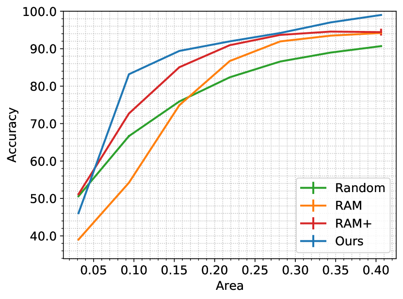
We compare our model with four baselines in Figure 2(a-e). RAM is a state-of-the-art hard attention model that observes images partially and sequentially to predict the class labels Mnih et al. (2014). We implement RAM using the same structure as our model. Instead of the Partial VAE, RAM has a controller that learns a Gaussian attention policy. Mnih et al. (2014) minimize at the end of steps. Following Li et al. (2017), we improve RAM by minimizing at all steps. We refer to this baseline as RAM+. We also consider a baseline model that attends glimpses on random locations. The Random baseline does not have a controller or a Partial VAE. Our model and the three baselines described so far observe the image only partially through a series of glimpses. Additionally, we train a feed-forward CNN that observes the entire image to predict the class label.
For the SVHN dataset, the Random baseline outperforms RAM for initial time steps. However, with time, RAM outperforms the Random baseline by attending more useful glimpses. RAM+ outperforms RAM and the Random baselines at all time steps. We observe a different trend for non-digit datasets. RAM+ consistently outperforms RAM on non-digit datasets; however, RAM+ falls behind the Random baseline. In RAM and RAM+, the classifier shares latent space with the controller, while the Random baseline dedicates an entire latent space to the classifier. We speculate that the dedicated latent space in the Random baseline is one of the reasons for its superior performance on complex datasets.

(a)

(b)

(c)

(d)

(e)

(f)

(a)

(b)

(c)

(d)

(e)

(f)

(a)

(b)

(c)

(d)
Our model consistently outperforms all attention baselines on all datasets. The performance gap between the highest performing baseline and our model reduces with many glimpses, as one can expect. Predicting an optimal glimpse-location is difficult for early time-steps as the models have access to minimal information about the scene so far. Compared to the highest performing baseline at , our model achieves around 10% higher accuracy on SVHN, around 5-6% higher accuracy on CIFAR-10 and CINIC-10, and around 2-3% higher accuracy on CIFAR-100 and TinyImageNet. Note that CIFAR-100 and TinyImageNet are more challenging datasets compared to SVHN, CINIC-10, and CIFAR-10. Similar to RAM and RAM+, the classifier and the Partial VAE share a common latent space in our model. Hence, our model achieves a lower gain over the Random baseline for complex datasets. We attribute the small but definite gain in the accuracy of our model to a better selection of glimpses.
The CNN has the highest accuracy as it observes a complete image. The accuracy of the CNN serves as the upper bound for the hard attention methods. Unlike CNN, the hard attention methods observe less than half of the image through small glimpses, each uncovering only 6.25% area of an image. On the CIFAR-10 dataset, the CNN predicts correct class labels for approximately 9 out of 10 images after observing each image completely. Remarkably, our model predicts correct class labels for 8 out of 10 images after observing less than half of the total area in each image.
4.1.1 Comparison of Attention Policies using a common CNN
Above, we compared the attention policies of various methods using their respective classifiers. However, each model attains different discriminative power due to different training objectives. While RAM, RAM+, and our model are trained jointly for two different tasks, i.e., classification and glimpse-location prediction or feature-synthesis, the Random baseline is trained for only one task, i.e., classification. Consequently, the Random baseline attains higher discriminative power than others and achieves high accuracy despite using a sub-optimal attention policy. To make a fair comparison of the attention policies irrespective of the discriminative power of the models, we perform the following experiment.
We mask all image regions except for the ones observed by the attention model so far and let the baseline CNN predict a class label from this masked image (see Figure 3). RAM+ consistently outperforms RAM, suggesting that the former has learned a better attention policy than the latter. As RAM+ is trained using at all time-steps, it achieves higher accuracy, and ultimately, higher reward during training with REINFORCE Mnih et al. (2014). RAM and RAM+ outperform the Random baseline for the SVHN dataset. However, they fall short on natural image datasets. In contrast, our method outperforms all baselines with a significant margin on all datasets, suggesting that the glimpses selected by our model are more informative about the image class than the ones chosen by the baselines.
RAM and RAM+ struggle on images with many objects and repeated structure Sermanet et al. (2014), as often the case with natural image datasets. For example, TinyImageNet includes many images with multiple objects (e.g. beer bottle), repeated patterns (e.g. spider web), and dispersed items (e.g. altar). Note that a random policy can perform competitively in such scenarios, especially when the location of various objects in an image is unknown due to partial observability. Yet, our method can learn policies that are superior to the Random baseline. Refer to SM for additional analyses.
4.2 Ablation study on Normalizing Flows
We inspect the necessity of a flexible distribution for the posterior and, therefore, the necessity of normalizing flows in the encoder . To this end, we model the posterior with a unimodal Gaussian distribution and let output mean and diagonal covariance of a Gaussian. We do not use flow layers in this case. Figure 2(f) shows the result for TinyImageNet dataset. We observe that modeling a complex posterior using normalizing flows improves accuracy. Ideally, the Partial VAE should predict all possibilities of consistent with the observed region . When the model observes a small region, a complex posterior helps determine multiple plausible feature maps. A unimodal posterior fails to cover all possibilities. Hence, the EIG estimated with the former is more accurate, leading to higher performance. Refer to SM for visualization of estimated with and without normalizing flows.
4.3 Visualization
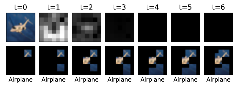
We visualize a few interesting examples of sequential recognition from the CIFAR-10 dataset in Figure 4. Refer to SM for additional examples. In Figure 4(a), activity in the map reduces as the model settles on a class ‘Bird’. In Figure 4(b), the model takes a long time to decide the true class of the image. Though incorrect, it predicts classes that are types of vehicles. After discovering parts like headlight and rear-view mirror, it predicts the true class ‘Automobile’ at . Figure 4(c) shows a difficult example. The model decides the true class ‘Bird’ after covering parts of the bird at . Notice a high amount of activity in the maps up to and reduced activity at . Figure 4(d) shows a failure case with enduring activity in maps. Finally, observe that the maps are often multimodal.
5 Conclusions
We presented a hard attention model that uses BOED to find the optimal locations to attend when the image is observed only partially. To find an optimal location without observing the corresponding glimpse, the model uses Partial VAE to synthesize the content of the glimpse in the feature space. Synthesizing features of unobserved regions is an ill-posed problem with multiple solutions. We use normalizing flows in Partial VAE to capture a complex distribution of unobserved glimpse features, which leads to improved performance. The synthesized features enable the model to evaluate and compare the expected information gain (EIG) of various candidate locations, from which the model selects a candidate with optimal EIG. The predicted EIG maps are often multimodal. Consequentially, the attention policy used by our model is multimodal. Our model achieves superior performance compared to the baseline methods that use unimodal attention policy, proving the effectiveness of multimodal policies in hard attention. When all models have seen only a couple of glimpses, our model achieves 2-10% higher accuracy than the baselines.
References
- Ahmad (1992) Subutai Ahmad. Visit: a neural model of covert visual attention. In Advances in neural information processing systems, pages 420–427, 1992.
- Alexe et al. (2012) Bogdan Alexe, Nicolas Heess, Yee W Teh, and Vittorio Ferrari. Searching for objects driven by context. In Advances in Neural Information Processing Systems, pages 881–889, 2012.
- Angles et al. (2018) Baptiste Angles, Simon Kornblith, Shahram Izadi, Andrea Tagliasacchi, and Kwang Moo Yi. Mist: Multiple instance spatial transformer network. arXiv preprint arXiv:1811.10725, 2018.
- Ba et al. (2014) Jimmy Ba, Volodymyr Mnih, and Koray Kavukcuoglu. Multiple object recognition with visual attention. arXiv preprint arXiv:1412.7755, 2014.
- Ba et al. (2015) Jimmy Ba, Russ R Salakhutdinov, Roger B Grosse, and Brendan J Frey. Learning wake-sleep recurrent attention models. In Advances in Neural Information Processing Systems, pages 2593–2601, 2015.
- Ba et al. (2016) Jimmy Lei Ba, Jamie Ryan Kiros, and Geoffrey E Hinton. Layer normalization. arXiv preprint arXiv:1607.06450, 2016.
- Bernardo (1979) José M Bernardo. Expected information as expected utility. the Annals of Statistics, pages 686–690, 1979.
- Butko and Movellan (2008) Nicholas J Butko and Javier R Movellan. I-pomdp: An infomax model of eye movement. In 2008 7th IEEE International Conference on Development and Learning, pages 139–144. IEEE, 2008.
- Butko and Movellan (2009) Nicholas J Butko and Javier R Movellan. Optimal scanning for faster object detection. In 2009 IEEE Conference on Computer Vision and Pattern Recognition, pages 2751–2758. IEEE, 2009.
- Cai and Wei (2020) Weiwei Cai and Zhanguo Wei. Piigan: Generative adversarial networks for pluralistic image inpainting. IEEE Access, 8:48451–48463, 2020.
- Chaloner and Verdinelli (1995) Kathryn Chaloner and Isabella Verdinelli. Bayesian experimental design: A review. Statistical Science, pages 273–304, 1995.
- Cordonnier et al. (2021) Jean-Baptiste Cordonnier, Aravindh Mahendran, Alexey Dosovitskiy, Dirk Weissenborn, Jakob Uszkoreit, and Thomas Unterthiner. Differentiable patch selection for image recognition. arXiv preprint arXiv:2104.03059, 2021.
- Darlow et al. (2018) Luke N Darlow, Elliot J Crowley, Antreas Antoniou, and Amos J Storkey. Cinic-10 is not imagenet or cifar-10. arXiv preprint arXiv:1810.03505, 2018.
- Denil et al. (2012) Misha Denil, Loris Bazzani, Hugo Larochelle, and Nando de Freitas. Learning where to attend with deep architectures for image tracking. Neural computation, 24(8):2151–2184, 2012.
- Dinh et al. (2016) Laurent Dinh, Jascha Sohl-Dickstein, and Samy Bengio. Density estimation using real nvp. arXiv preprint arXiv:1605.08803, 2016.
- Durkan et al. (2019) Conor Durkan, Artur Bekasov, Iain Murray, and George Papamakarios. Neural spline flows. In Advances in Neural Information Processing Systems, pages 7511–7522, 2019.
- Elsayed et al. (2019) Gamaleldin Elsayed, Simon Kornblith, and Quoc V Le. Saccader: improving accuracy of hard attention models for vision. In Advances in Neural Information Processing Systems, pages 702–714, 2019.
- Eslami et al. (2016) SM Ali Eslami, Nicolas Heess, Theophane Weber, Yuval Tassa, David Szepesvari, Geoffrey E Hinton, et al. Attend, infer, repeat: Fast scene understanding with generative models. In Advances in Neural Information Processing Systems, pages 3225–3233, 2016.
- Garnelo et al. (2018a) Marta Garnelo, Dan Rosenbaum, Christopher Maddison, Tiago Ramalho, David Saxton, Murray Shanahan, Yee Whye Teh, Danilo Rezende, and SM Ali Eslami. Conditional neural processes. In International Conference on Machine Learning, pages 1704–1713, 2018a.
- Garnelo et al. (2018b) Marta Garnelo, Jonathan Schwarz, Dan Rosenbaum, Fabio Viola, Danilo J Rezende, SM Eslami, and Yee Whye Teh. Neural processes. arXiv preprint arXiv:1807.01622, 2018b.
- Gregor et al. (2015) Karol Gregor, Ivo Danihelka, Alex Graves, Danilo Jimenez Rezende, and Daan Wierstra. Draw: A recurrent neural network for image generation. In ICML, 2015.
- Harvey et al. (2019) William Harvey, Michael Teng, and Frank Wood. Near-optimal glimpse sequences for improved hard attention neural network training. arXiv preprint arXiv:1906.05462, 2019.
- Huang et al. (2018) Sheng-Jun Huang, Miao Xu, Ming-Kun Xie, Masashi Sugiyama, Gang Niu, and Songcan Chen. Active feature acquisition with supervised matrix completion. In Proceedings of the 24th ACM SIGKDD International Conference on Knowledge Discovery & Data Mining, pages 1571–1579, 2018.
- Iizuka et al. (2017) Satoshi Iizuka, Edgar Simo-Serra, and Hiroshi Ishikawa. Globally and locally consistent image completion. ACM Transactions on Graphics (ToG), 36(4):1–14, 2017.
- Ilse et al. (2018) Maximilian Ilse, Jakub Tomczak, and Max Welling. Attention-based deep multiple instance learning. In International conference on machine learning, pages 2127–2136. PMLR, 2018.
- Ioffe and Szegedy (2015) Sergey Ioffe and Christian Szegedy. Batch normalization: Accelerating deep network training by reducing internal covariate shift. arXiv preprint arXiv:1502.03167, 2015.
- Itti and Baldi (2006) Laurent Itti and Pierre F Baldi. Bayesian surprise attracts human attention. In Advances in neural information processing systems, pages 547–554, 2006.
- Itti and Koch (2000) Laurent Itti and Christof Koch. A saliency-based search mechanism for overt and covert shifts of visual attention. Vision research, 40(10-12):1489–1506, 2000.
- Itti et al. (1998) Laurent Itti, Christof Koch, and Ernst Niebur. A model of saliency-based visual attention for rapid scene analysis. IEEE Transactions on pattern analysis and machine intelligence, 20(11):1254–1259, 1998.
- Jaderberg et al. (2015) Max Jaderberg, Karen Simonyan, Andrew Zisserman, et al. Spatial transformer networks. In Advances in neural information processing systems, pages 2017–2025, 2015.
- Katharopoulos and Fleuret (2019) Angelos Katharopoulos and Francois Fleuret. Processing megapixel images with deep attention-sampling models. In International Conference on Machine Learning, pages 3282–3291, 2019.
- Kingma and Ba (2014) Diederik P Kingma and Jimmy Ba. Adam: A method for stochastic optimization. arXiv preprint arXiv:1412.6980, 2014.
- Kingma and Welling (2013) Diederik P Kingma and Max Welling. Auto-encoding variational bayes. arXiv preprint arXiv:1312.6114, 2013.
- Kingma and Dhariwal (2018) Durk P Kingma and Prafulla Dhariwal. Glow: Generative flow with invertible 1x1 convolutions. In Advances in neural information processing systems, pages 10215–10224, 2018.
- Kingma et al. (2016) Durk P Kingma, Tim Salimans, Rafal Jozefowicz, Xi Chen, Ilya Sutskever, and Max Welling. Improved variational inference with inverse autoregressive flow. In Advances in neural information processing systems, pages 4743–4751, 2016.
- Koch and Ullman (1987) Christof Koch and Shimon Ullman. Shifts in selective visual attention: towards the underlying neural circuitry. In Matters of intelligence, pages 115–141. Springer, 1987.
- Krizhevsky et al. (2009) Alex Krizhevsky et al. Learning multiple layers of features from tiny images. 2009.
- Larochelle and Hinton (2010) Hugo Larochelle and Geoffrey E Hinton. Learning to combine foveal glimpses with a third-order boltzmann machine. In Advances in neural information processing systems, pages 1243–1251, 2010.
- Li et al. (2016) Fei-Fei Li, Andrej Karpathy, and Justin Johnson. Tiny imagenet challenge. http://cs231n.stanford.edu/2016/project.html, 2016.
- Li et al. (2017) Zhichao Li, Yi Yang, Xiao Liu, Feng Zhou, Shilei Wen, and Wei Xu. Dynamic computational time for visual attention. In Proceedings of the IEEE International Conference on Computer Vision Workshops, pages 1199–1209, 2017.
- Lin et al. (2017) Zhouhan Lin, Minwei Feng, Cicero Nogueira dos Santos, Mo Yu, Bing Xiang, Bowen Zhou, and Yoshua Bengio. A structured self-attentive sentence embedding. In International Conference on Learning Representations, 2017.
- Lindley (1956) Dennis V Lindley. On a measure of the information provided by an experiment. The Annals of Mathematical Statistics, pages 986–1005, 1956.
- Lu (2019) Jialin Lu. Revisit recurrent attention model from an active sampling perspective. NeuroAI workshop, NeurIPS, 2019.
- Ma et al. (2018) Chao Ma, Sebastian Tschiatschek, Konstantina Palla, José Miguel Hernández-Lobato, Sebastian Nowozin, and Cheng Zhang. Eddi: Efficient dynamic discovery of high-value information with partial vae. arXiv preprint arXiv:1809.11142, 2018.
- Melville et al. (2004) Prem Melville, Maytal Saar-Tsechansky, Foster Provost, and Raymond Mooney. Active feature-value acquisition for classifier induction. In Fourth IEEE International Conference on Data Mining (ICDM’04), pages 483–486. IEEE, 2004.
- Mnih et al. (2014) Volodymyr Mnih, Nicolas Heess, Alex Graves, et al. Recurrent models of visual attention. In Advances in neural information processing systems, pages 2204–2212, 2014.
- Netzer et al. (2011) Yuval Netzer, Tao Wang, Adam Coates, Alessandro Bissacco, Bo Wu, and Andrew Y Ng. Reading digits in natural images with unsupervised feature learning. Advances in neural information processing systems, 2011.
- Olshausen et al. (1993) Bruno A Olshausen, Charles H Anderson, and David C Van Essen. A neurobiological model of visual attention and invariant pattern recognition based on dynamic routing of information. Journal of Neuroscience, 13(11):4700–4719, 1993.
- Paletta et al. (2005) Lucas Paletta, Gerald Fritz, and Christin Seifert. Q-learning of sequential attention for visual object recognition from informative local descriptors. In Proceedings of the 22nd international conference on Machine learning, pages 649–656, 2005.
- Papadopoulos et al. (2021) Athanasios Papadopoulos, Paweł Korus, and Nasir Memon. Hard-attention for scalable image classification. arXiv preprint arXiv:2102.10212, 2021.
- Pathak et al. (2016) Deepak Pathak, Philipp Krahenbuhl, Jeff Donahue, Trevor Darrell, and Alexei A Efros. Context encoders: Feature learning by inpainting. In Proceedings of the IEEE conference on computer vision and pattern recognition, pages 2536–2544, 2016.
- Ranzato (2014) Marc’Aurelio Ranzato. On learning where to look. arXiv preprint arXiv:1405.5488, 2014.
- Ren et al. (2015) Shaoqing Ren, Kaiming He, Ross Girshick, and Jian Sun. Faster r-cnn: towards real-time object detection with region proposal networks. In Proceedings of the 28th International Conference on Neural Information Processing Systems-Volume 1, pages 91–99, 2015.
- Rimey and Brown (1991) Raymond D Rimey and Christopher M Brown. Controlling eye movements with hidden markov models. International Journal of Computer Vision, 7(1):47–65, 1991.
- Schwartenbeck et al. (2013) Philipp Schwartenbeck, Thomas FitzGerald, Ray Dolan, and Karl Friston. Exploration, novelty, surprise, and free energy minimization. Frontiers in psychology, 4:710, 2013.
- Sermanet et al. (2014) Pierre Sermanet, Andrea Frome, and Esteban Real. Attention for fine-grained categorization. arXiv preprint arXiv:1412.7054, 2014.
- Sohn et al. (2015) Kihyuk Sohn, Honglak Lee, and Xinchen Yan. Learning structured output representation using deep conditional generative models. Advances in neural information processing systems, 28:3483–3491, 2015.
- Tang et al. (2014) Charlie Tang, Nitish Srivastava, and Russ R Salakhutdinov. Learning generative models with visual attention. In Advances in Neural Information Processing Systems, pages 1808–1816, 2014.
- Uzkent and Ermon (2020) Burak Uzkent and Stefano Ermon. Learning when and where to zoom with deep reinforcement learning. In Proceedings of the IEEE/CVF Conference on Computer Vision and Pattern Recognition, pages 12345–12354, 2020.
- Van der Maaten and Hinton (2008) Laurens Van der Maaten and Geoffrey Hinton. Visualizing data using t-sne. Journal of machine learning research, 9(11), 2008.
- Wang et al. (2014) Miao Wang, Yu-Kun Lai, Yuan Liang, Ralph R Martin, and Shi-Min Hu. Biggerpicture: data-driven image extrapolation using graph matching. ACM Transactions on Graphics, 33(6), 2014.
- Wang et al. (2019) Yi Wang, Xin Tao, Xiaoyong Shen, and Jiaya Jia. Wide-context semantic image extrapolation. In Proceedings of the IEEE/CVF Conference on Computer Vision and Pattern Recognition, pages 1399–1408, 2019.
- Xu et al. (2015) Kelvin Xu, Jimmy Ba, Ryan Kiros, Kyunghyun Cho, Aaron Courville, Ruslan Salakhudinov, Rich Zemel, and Yoshua Bengio. Show, attend and tell: Neural image caption generation with visual attention. In International conference on machine learning, pages 2048–2057, 2015.
- Yang et al. (2019) Zongxin Yang, Jian Dong, Ping Liu, Yi Yang, and Shuicheng Yan. Very long natural scenery image prediction by outpainting. In Proceedings of the IEEE/CVF International Conference on Computer Vision, pages 10561–10570, 2019.
- Yu et al. (2018) Jiahui Yu, Zhe Lin, Jimei Yang, Xiaohui Shen, Xin Lu, and Thomas S Huang. Generative image inpainting with contextual attention. In Proceedings of the IEEE conference on computer vision and pattern recognition, pages 5505–5514, 2018.
- Zhang et al. (2020) Lingzhi Zhang, Jiancong Wang, and Jianbo Shi. Multimodal image outpainting with regularized normalized diversification. In Proceedings of the IEEE/CVF Winter Conference on Applications of Computer Vision, pages 3433–3442, 2020.
- Zhao et al. (2020) Lei Zhao, Qihang Mo, Sihuan Lin, Zhizhong Wang, Zhiwen Zuo, Haibo Chen, Wei Xing, and Dongming Lu. Uctgan: Diverse image inpainting based on unsupervised cross-space translation. In Proceedings of the IEEE/CVF Conference on Computer Vision and Pattern Recognition, pages 5741–5750, 2020.
- Zheng et al. (2019) Chuanxia Zheng, Tat-Jen Cham, and Jianfei Cai. Pluralistic image completion. In Proceedings of the IEEE/CVF Conference on Computer Vision and Pattern Recognition, pages 1438–1447, 2019.
- Zheng et al. (2015) Yin Zheng, Richard S Zemel, Yu-Jin Zhang, and Hugo Larochelle. A neural autoregressive approach to attention-based recognition. International Journal of Computer Vision, 113(1):67–79, 2015.
Appendix A Architecture
Table 1 shows the architecture of various components of our model. Note that all modules use a small number of layers. uses the least possible layers to achieve the effective receptive field equal to the area of a single glimpse. The decoder uses the smallest number of and layers to generate the feature maps of required spatial dimensions and refine them based on the global context. The encoder uses flow layers according to the complexity of the dataset. All other modules use a single linear layer. We implement linear layers using convolution layers. The dimensionality of features , hidden state and latent representation for various datasets are mentioned in Table 2.
| Module | Architecture | |
|---|---|---|
| Recurrent feature aggregator | ||
| Classifier | ||
| Partial VAE | ||
| SVHN | 128 | 512 | 256 |
|---|---|---|---|
| CINIC-10 | 128 | 512 | 256 |
| CIFAR-10 | 128 | 512 | 256 |
| CIFAR-100 | 512 | 2048 | 1024 |
| TinyImageNet | 512 | 2048 | 1024 |
Appendix B Optimization Details
We train our model in three stages until convergence. In the first stage we pre-train , and . In the second stage, we pre-train and while keeping , , and frozen. In the third stage, we finetune all modules end-to-end. Unless stated otherwise, we use the same setting for all three stages. We trained our models on a single Tesla P100 GPU with 12GB of memory or a single Tesla V100 GPU with 16GB of memory.
Data Preparation. We augment training images using random crop, scale, horizontal flip and color jitter transformations, and map pixel values in range . We use a batch-size of 64. We use the same scheme for all datasets.
Loss Function. We compute an average loss across batch and time. We set the hyperparameters and of the loss function as follows. The hyperparameter is set to the inverse of dimensionality of the latent representation . The hyperparameter is set to 32, 16, 16, 8 and 8 for SVHN, CINIC-10, CIFAR-10, CIFAR-100 and TinyImageNet respectively.
Optimizer. We use Adam optimizer Kingma and Ba (2014) with the default setting of . In the first training stage, we use a learning rate of 0.001 for all datasets. In the second and third training stages, we use a learning rate of 0.001 for SVHN, CIFAR-10, and CINIC-10, and a learning rate of 0.0001 for CIFAR-100 and TinyImageNet. We divide the learning rate by 0.5 at a plateau.
(a)

(b)

(c)

(d)

(e)

(a)

(b)

(c)

(d)

(e)

(a)

(b)

(c)

(d)

(e)

t=0


t=1


t=2


t=3


t=4


t=5


(a)

(b)


Airplane Automobile Bird Cat Deer Dog Frog Horse Ship Truck
Appendix C Additional Experiments
C.1 Accuracy as a function of area observed in an image
At a time, a hard attention model observes only a small region of the input image through a glimpse. As time progresses, the model observes more area in the image through multiple glimpses. We compare the accuracy of various models as a function of the area observed in an image (see Figure 5). RAM+ consistently outperforms RAM on various datasets. We observe that the Random baseline performs better than the RAM and RAM+ on comparatively more challenging datasets. As discussed in the main paper, the Random baseline dedicates an entire latent space to the classifier. Our model, RAM+, and RAM use a common latent space for a classifier and a Partial VAE or a controller. Finally, for any given value of the observed area, our model achieves the highest accuracy. The result suggests that our model captures glimpses on the regions that provide more useful information about the class label than the baseline methods.
C.2 Entropy in the class-logits as a function of number of glimpses
An efficient hard attention model should become more confident in predicting a class label with small number of glimpses. We measure confidence using entropy in the predicted class-logits; lower entropy indicates higher confidence. Figure 6 shows entropy in the class-logits predicted by various models with time. Irrespective of the glimpse acquisition strategy, all models reduce entropy in their predictions as they acquire more glimpses. In case of RAM, the trend is inconsistent for initial time steps. Recall that RAM optimizes loss only at the last time step, unlike other models that optimize losses for all time steps. Consistent with the previous analyses, RAM+ outperforms RAM on all datasets, and the Random baseline outperforms RAM and RAM+ on complex datasets. Our model achieves lower entropy with smaller number of glimpses compared to the baseline methods. The result indicates that our model acquires glimpses that help the most in reducing the uncertainty in the class-label prediction.
C.3 Generalization to a large number of glimpses
Recall that all models are trained for seven glimpses. In Figure 7, we assess their inference-time generalizability for a large number of glimpses by testing the models for T=49. Note that our method would have observed an entire image by then. We notice that, during the inference-time, RAM does not generalize well to a sequence of glimpses that are longer than the training time; Elsayed et al. (2019); Sermanet et al. (2014); Lu (2019) also make a similar observation. Our method and RAM+ show greater generalizability than RAM. While the Random baseline is the most generalizable, our method outperforms it with an optimal number of glimpses. The accuracy achieved by our model with an optimal number of glimpses is lower than the CNN; however, the CNN is trained exclusively on complete images, and our model is not. Note that the primary motivation for the attention mechanism is to achieve higher accuracy using limited time and constrained resources. If time and resources are available, one can instead collect a large number of random glimpses and use a non-attentive CNN.


C.4 Visualization of estimated with and without normalizing flows
Synthesizing a feature map of a complete image using only partial observations is an ill-posed problem with many solutions. We use normalizing flows in the encoder to capture a complex multimodal posterior that helps the decoder predict multiple plausible feature maps for a complete image. We perform an ablation study to analyze the importance of using normalizing flows. In Figure 8, we present TSNE Van der Maaten and Hinton (2008) projections of estimated with and without the use of normalizing flows. We can observe that the normalizing flows capture a complex multimodal posterior. Capturing multiple modes leads to a more accurate estimation of EIG and consequently higher performance.
C.5 Self-attention in
Here, we experiment with self-attention in . We adapt the method proposed in Lin et al. (2017) for our problem. Figure 9(a) compares the performance of our model with and without self-attention. We observe only a marginal performance improvement due to self-attention, perhaps because the sequence of seven glimpses is relatively short. However, self-attention may achieve higher accuracy if the model is trained for longer sequences. Nevertheless, the results of this preliminary experiment are favorable, suggesting that exploring self-attention in is a promising direction for future works.
C.6 Confusion matrix
In Figure 10, we display the confusion matrix of various methods for the CIFAR-10 dataset at t=6. We also show the average image for each class. We observe that the models are able to discern classes with similar color schemes, suggesting that they rely on complex high level features instead of simple low level features such as pixel color. Furthermore, the Random baseline, the RAM, and the RAM+ over-represent category ‘frog’, confusing it with many other categories. Our method does not suffer from this phenomenon.
C.7 Additional visualization
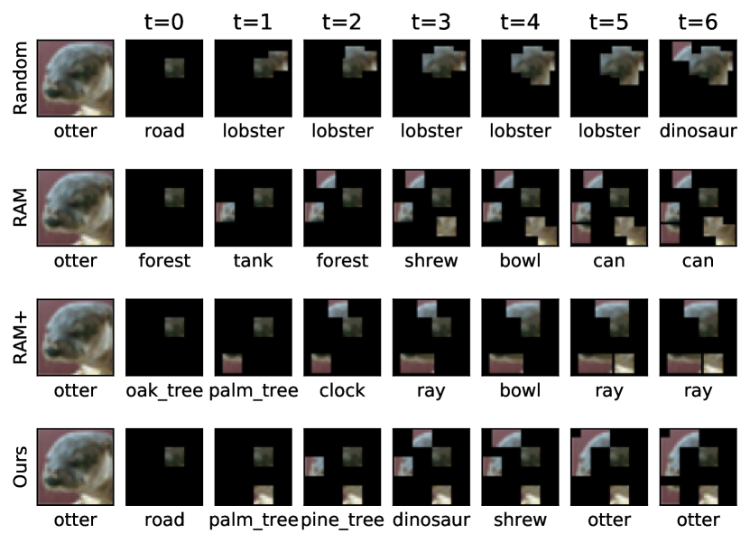
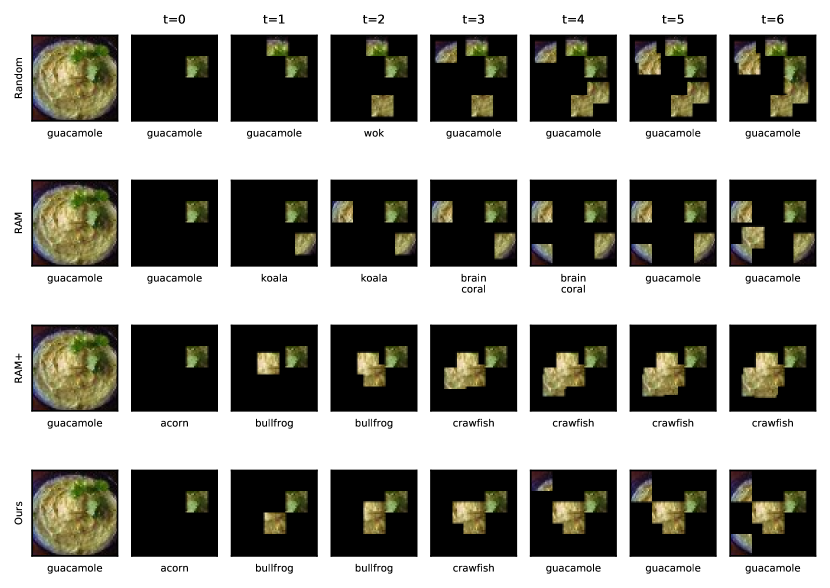
In Figure 11-13, we visualize the maps and the glimpses observed by our model on CIFAR-10 images. The top rows in each plot show the entire image and the maps for to 6. The bottom rows in each plot show glimpses attended by our model. The model observes the first glimpse at a random location. Our model observes a glimpse of size . The glimpses overlap with the stride of 4, resulting in a grid of glimpses. The EIG maps are of size and are upsampled for the display. We display the entire image for reference; our model never observes the whole image. Additionally, in Figure 14-16, we visualize a series of glimpses selected by various models for one image from all datasets. A complete image is shown for reference. Compared methods do not observe the complete image. Ground Truth label is shown in the first column, below the complete image. Labels predicted after observing various glimpses are shown in the columns marked with time .
Appendix D Normalizing Flows
Normalizing Flows map a Gaussian distribution to a complex multi-modal distribution using a series of differentiable and invertible functions. We use conditional normalizing flows that map samples from (Gaussian distribution) to (a complex distribution) using a series of invertible functions conditioned on .
| (8) |
The relation between and is established using a change of variable formula.
| (9) |
Where is a Jacobian of . We use , where values of are given in Table 1. For all , we define and using ActNorm Kingma and Dhariwal (2018), Flip Dinh et al. (2016) and Neural Spline Flows Durkan et al. (2019), respectively. Below, we provide a brief introduction on these three functions. To reduce clutter, we refer to as and as .
ActNorm Kingma and Dhariwal (2018). An ActNorm layer performs an element-wise scaling and shifting of .
| (10) |
The scale parameter and the shift parameter are predicted by a neural network using . We adapt a data-dependent initialization scheme for this network Kingma and Dhariwal (2018). Specifically, we initialize the above neural network such that the predicted and yield with unit variance and zero mean for the first batch. We can compute .
Flip Dinh et al. (2016). A Flip layer simply reverses elements of , i.e. . The Jacobian determinant .
Neural Spline Flows (NSF) Durkan et al. (2019). An NSF performs element-wise transformations on . Specifically, it transforms an element using a monotonic piece-wise spline function that is defined using parameters . Refer to Durkan et al. (2019) for more details on these parameters. In auto-regressive NSF, a neural network predicts the parameters of from the elements and . Then, we find a specific for which and transform as follows.
| (11) | ||||
| (12) | ||||
| (13) |
The derivative of is defined as follows.
| (14) |
As NSF applies element-wise monotonic functions, .