A Practical, Progressively-Expressive GNN
Abstract
Message passing neural networks (MPNNs) have become a dominant flavor of graph neural networks (GNNs) in recent years. Yet, MPNNs come with notable limitations; namely, they are at most as powerful as the 1-dimensional Weisfeiler-Leman (1-WL) test in distinguishing graphs in a graph isomorphism testing framework. To this end, researchers have drawn inspiration from the -WL hierarchy to develop more expressive GNNs. However, current -WL-equivalent GNNs are not practical for even small values of , as -WL becomes combinatorially more complex as grows. At the same time, several works have found great empirical success in graph learning tasks without highly expressive models, implying that chasing expressiveness with a “coarse-grained ruler” of expressivity like -WL is often unneeded in practical tasks. To truly understand the expressiveness-complexity tradeoff, one desires a more “fine-grained ruler,” which can more gradually increase expressiveness. Our work puts forth such a proposal: Namely, we first propose the -SetWL hierarchy with greatly reduced complexity from -WL, achieved by moving from -tuples of nodes to sets with nodes defined over connected components in the induced original graph. We show favorable theoretical results for this model in relation to -WL, and concretize it via -SetGNN, which is as expressive as -SetWL. Our model is practical and progressively-expressive, increasing in power with and . We demonstrate effectiveness on several benchmark datasets, achieving several state-of-the-art results with runtime and memory usage applicable to practical graphs. We open source our implementation at https://github.com/LingxiaoShawn/KCSetGNN.
1 Introduction
In recent years, graph neural networks (GNNs) have gained considerable attention [58, 60] for their ability to tackle various node-level [35, 56], link-level [66, 51] and graph-level [9, 40] learning tasks, given their ability to learn rich representations for complex graph-structured data. The common template for designing GNNs follows the message passing paradigm; these so-called message-passing neural networks (MPNNs) are built by stacking layers which encompass feature transformation and aggregation operations over the input graph [39, 25]. Despite their advantages, MPNNs have several limitations including oversmoothing [67, 12, 47], oversquashing [2, 55], inability to distinguish node identities [63] and positions [62], and expressive power [61].
Since Xu et al.’s [61] seminal work showed that MPNNs are at most as powerful as the first-order Weisfeiler-Leman (1-WL) test in the graph isomorphism (GI) testing framework, there have been several follow-up works on improving the understanding of GNN expressiveness [3, 15]. In response, the community proposed many GNN models to overcome such limitations [52, 4, 68]. Several of these aim to design powerful higher-order GNNs which are increasingly expressive [43, 41, 33, 9] by inspiration from the -WL hierarchy [54].
A key limitation of such higher-order models that reach beyond 1-WL is their poor scalability; in fact, these models can only be applied to small graphs with small in practice [40, 41, 43] due to combinatorial growth in complexity. On the other hand lies an open question on whether practical graph learning tasks indeed need such complex, and extremely expressive GNN models. Historically, Babai et al. [5] showed that almost all graphs on nodes can be distinguished by 1-WL. In other contexts like node classification, researchers have encountered superior generalization performance with graph-augmented multi-layer perceptron (GA-MLP) models [50, 37] compared to MPNNs, despite the former being strictly less expressive than the latter [13]. Considering that increased model complexity has negative implications in terms of overfitting and generalization [29], it is worth re-evaluating continued efforts to pursue maximally expressive GNNs in practice. Ideally, one could study these models’ generalization performance on various real-world tasks by increasing (expressiveness) in the -WL hierarchy. Yet, given the impracticality of this too-coarse “ruler” of expressiveness, which becomes infeasible beyond , one desires a more fine-grained “ruler”, that is, a new hierarchy whose expressiveness grows more gradually. Such a hierarchy could enable us to gradually build more expressive models which admit improved scaling, and avoid unnecessary leaps in model complexity for tasks which do not require them, guarding against overfitting.

Present Work. In this paper, we propose such a hierarchy, and an associated practical progressively-expressive GNN model, called -SetGNN, whose expressiveness can be modulated through and . In a nutshell, we take inspiration from -WL, yet achieve practicality through three design ideas which simplify key bottlenecks of scaling -WL: First, we move away from -tuples of the original -WL to -multisets (unordered), and then to -sets. We demonstrate that these steps drastically reduce the number nodes in the -WL graph while retaining significant expressiveness. (Sec.s 3.23.3) Second, by considering the underlying sparsity of an input graph, we reduce scope to -sets that consist of nodes whose induced subgraph is comprised of connected components. This also yields massive reduction in the number of nodes while improving practicality; i.e. small values of on sparse graphs can allow one to increase well beyond in practice. (Sec. 3.4) Third, we design a super-graph architecture that consists of a sequence of bipartite graphs over which we learn embeddings for our -sets, using bidirectional message passing. These embeddings can be pooled to yield a final graph embedding.. (Sec.s 4.14.2) We also speed up initializing “colors” for the -sets, for , substantially reducing computation and memory. (Sec. 4.3) Fig. 1 overviews of our proposed framework. Experimentally, our -SetGNN outperforms existing state-of-the-art GNNs on simulated expressiveness as well as real-world graph-level tasks, achieving new bests on substructure counting and ZINC-12K, respectively. We show that generalization performance reflects increasing expressiveness by and . Our proposed scalable designs allow us to train models with e.g. or with practical running time and memory requirements.
2 Related Work
MPNN limitations. Given the understanding that MPNNs have expressiveness upper-bounded by 1-WL [61], several researchers investigated what else MPNNs cannot learn. To this end, Chen et al. [15] showed that MPNNs cannot count induced connected substructures of 3 or more nodes, while along with [15], Arvind et al. [3] showed that MPNNs can only count star-shaped patterns. Loukas [38] further proved several results regarding decision problems on graphs (e.g. subgraph verification, cycle detection), finding that MPNNs cannot solve these problems unless strict conditions of depth and width are met. Moreover, Garg et al. [22] showed that many standard MPNNs cannot compute properties such as longest or shortest cycles, diameters or existence of cliques.
Improving expressivity. Several works aim to improve expressiveness limitations of MPNNs. One approach is to inject features into the MPNN aggregation, motivated by Loukas [38] who showed that MPNNs can be universal approximators when nodes are sufficiently distinguishable. Sato et al. [53] show that injecting random features can better enable MPNNs to solve problems like minimum dominating set and maximum matching. You et al. [63] inject cycle counts as node features, motivated by the limitation of MPNNs not being able to count cycles. Others proposed utilizing subgraph isomorphism counting to empower MPNNs with substructure information they cannot learn [10, 9]. Earlier work by You et al. [62] adds positional features to distinguish node which naïve MPNN embeddings would not. Recently, several works also propose utilizing subgraph aggregation; Zhang et al. [65], Zhao et al. [68] and Bevilacqua et al. [8] propose subgraph variants of the WL test which are no less powerful than 3-WL. Recently a following up work [21] shows that rooted subgraph based extension with 1-WL as kernel is bounded by 3-WL. The community is yet exploring several distinct avenues in overcoming limitations: Murphy et al. [46] propose a relational pooling mechanism which sums over all permutations of a permutation-sensitive function to achieve above-1-WL expressiveness. Balcilar et al. [6] generalizes spatial and spectral MPNNs and shows that instances of spectral MPNNs are more powerful than 1-WL. Azizian et al. [4] and Geerts et al. [24] unify expressivity and approximation ability results for existing GNNs.
-WL-inspired GNNs. The -WL test captures higher-order interactions in graph data by considering all -tuples, i.e., size ordered multisets defined over the set of nodes. While highly expressive, it does not scale to practical graphs beyond a very small ( pushes the practical limit even for small graphs). However, several works propose designs which can achieve -WL in theory and strive to make them practical. Maron et al. [41] proposes a general class of invariant graph networks -IGNs having exact -WL expressivity [23], while being not scalable. Morris et al. have several work on -WL and its variants like -LWL [42], -GNN [43], and --WL-GNN [44]. Both -LWL and -GNN use a variant of -WL that only considers -sets and are strictly weaker than -WL but much more practical. In our paper we claim that -sets should be used with additional designs to keep the best expressivity while remaining practical. The --WL-GNN works with -tuples but sparsifies the connections among tuples by considering locality. Qian et al. [48] extends the k-tuple to subgraph network but has same scalability bottleneck as k-WL. A recent concurrent work SpeqNet [45] proposes to reduce number of tuples by restricting the number of connected components of tuples’ induced subgraphs. The idea is independently explored in our paper in Sec.3.4. All four variants proposed by Morris et al. do not have realizations beyond in their experiments while we manage to reach . Interestingly, a recent work [34] links graph transformer with -IGN that having better (or equal) expressivity, however is still not scalable.
3 A practical progressively-expressive isomorphism test: -SetWL
We first motivate our method -SetGNN from the GI testing perspective by introducing -SetWL. We first introduce notation and background of -WL (Sec. 3.1). Next, we show how to increase the practicality of -WL without reducing much of its expressivity, by removing node ordering (Sec. 3.2), node repetitions (Sec. 3.3), and leveraging graph sparsity (Sec. 3.4). We then give the complexity analysis (Sec. 3.5). We close the section with extending the idea to -FWL which is as expressive as +-WL (Sec. 3.6). All proofs are included in Appendix A.4.
Notation: Let be an undirected, colored graph with nodes , edges , and a color-labeling function where denotes a set of distinct colors. Let . Let denote a tuple (ordered multiset), denote a multiset (set which allows repetition), and denote a set. We define as a -tuple, as a -multiset, and as a -set. Let denote replacing the -th element in with , and analogously for and (assume mutlisets and sets are represented with the canonical ordering). When , let , , denote the induced subgraph on with nodes inside respectively (keeping repetitions). An isomorphism between two graphs and is a bijective mapping which satisfies and . Two graphs are isomorphic if there exists an isomorphism between them, which we denote as .
3.1 Preliminaries: the -Weisfeiler-Leman (-WL) Graph Isomorphism Test
The 1-dimensional Weisfeiler-Leman (-WL) test, also known as color refinement [49] algorithm, is a widely celebrated approach to (approximately) test GI. Although extremely fast and effective for most graphs (-WL can provide canonical forms for all but fraction of -vertex graphs [5]), it fails to distinguish members of many important graph families, such as regular graphs. The more powerful -WL algorithm first appeared in [57], and extends coloring of vertices (or 1-tuples) to that of -tuples. -WL is progressively expressive with increasing , and can distinguish any finite set of graphs given a sufficiently large . -WL has many interesting connections to logic, games, and linear equations [11, 28]. Another variant of -WL is called -FWL (Folklore WL), such that -WL is equally expressive as -FWL [11, 26]. Our work focuses on -WL.
-WL iteratively recolors all -tuples defined on a graph with nodes. At iteration 0, each -tuple is initialized with a color as its atomic type . Assume has colors, then is an ordered vector encoding. The first entries indicate whether , , which is the node repetition information. The second entries indicate whether . The last entries one-hot encode the initial color of , . Importantly, if and only if is an isomorphism from to . Let denote the color of -tuple on graph at -th iteration of -WL, where colors are initialized with .
At the -th iteration, -WL updates the color of each according to
| (1) |
Let denote the encoding of at -th iteration of -WL. Then,
| (2) |
Two -tuples and are connected by an edge if , or informally if they share entries. Then, -WL defines a super-graph with its nodes being all -tuples in , and edges defined as above. Eq. (1) defines the rule of color refinement on . Intuitively, -WL is akin to (but more powerful as it orders subgroups of neighbors) running 1-WL algorithm on the supergraph . As , the color converges to a stable value, denoted as and the corresponding stable graph color denoted as . For two non-isomorphic graphs , -WL can successfully distinguish them if . The expressivity of can be exactly characterized by first-order logic with counting quantifiers. Let denote all first-order formulas with at most variables and -depth counting quantifiers, then . Additionally, there is a -step bijective pebble game that are equivalent to -iteration -WL in expressivity. See Appendix.A.2 for the pebble game characterization of -WL.
Despite its power, -WL uses all tuples and has complexity at each iteration.
3.2 From -WL to -MultisetWL: Removing Ordering
Our first proposed adaptation to -WL is to remove ordering in each -tuple, i.e. changing -tuples to -multisets. This greatly reduces the number of supernodes to consider by times.
Let be the corresponding multiset of tuple . We introduce a canonical order function on , , and a corresponding indexing function , which returns the -th element of sorted according to . Let denote the color of the -multiset at -th iteration of -MultisetWL, formally defined next.
At , we initialize the color of as where perm[k]111This function should also consider repeated elements; we omit this for clarity of presentation. denotes the set of all permutation mappings of elements. It can be shown that if and only if and are isomorphic.
At -th iteration, -MultisetWL updates the color of every -multiset by
| (3) | ||||
Where denotes replacing the -th (ordered by ) element of the multiset with . Let denote the super-graph defined by -MultisetWL. Similar to Eq. (2), the graph level encoding is .
Interestingly, although -MultisetWL has significantly fewer number of node groups than -WL, we show it is no less powerful than --WL in terms of distinguishing graphs, while being upper bounded by -WL in distingushing both node groups and graphs.
Theorem 1.
Let and . For all and all graphs : -MultisetWL is upper bounded by -WL in distinguishing multisets and at -th iteration, i.e. .
Theorem 2.
-MultisetWL is no less powerful than (-)-WL in distinguishing graphs: for any there exists graphs that can be distinguished by -MultisetWL but not by (-)-WL.
Theorem 2 is proved by using a variant of a series of CFI [11] graphs which cannot be distinguished by -WL. This theorem shows that -MultisetWL is indeed very powerful and finding counter examples of -WL distinguishable graphs that cannot be distinguished by -MultisetWL is very hard. Hence we conjecture that -MultisetWL may have the same expressivity as -WL in distinguishing undirected graphs, with an attempt of proving it in Appendix.A.4.10. Additionally, the theorem also implies that -MultisetWL is strictly more powerful than ()-MultisetWL.
We next give a pebble game characterization of -MultisetWL, which is named doubly bijective -pebble game presented in Appendix.A.3. The game is used in the proof of Theorem 2.
Theorem 3.
-MultisetWL has the same expressivity as the doubly bijective -pebble game.
3.3 From -MultisetWL to -SetWL: Removing Repetition
Next, we propose further removing repetition inside any -multiset, i.e. transforming -multisets to -sets. We assume elements of -multiset and -set in are sorted based on the ordering function , and omit for clarity. Let transform a multiset to set by removing repeats, and let return a tuple with the number of repeats for each distinct element in a multiset. Specifically, let and , then denotes the number of distinct elements in -multiset , and , is the -th distinct element with repetitions. Clearly there is an injective mapping between and ; let be the inverse mapping such that . Equivalently, each -set can be mapped with a multiset of -multisets: . Based on this relationship, we extend the connection among -multisets to -sets: given , a -set is connected to a -set if and only if , is connected with in -MultisetWL. Let denote the defined super-graph on by -SetWL. It can be shown that this is equivalent to either (1) or (2) is true. Notice that contains a sequence of bipartite graphs with each reflecting the connections among the ()-sets and the -sets. It also contains subgraphs, i.e. the connections among the -sets for . Later on we will show that these subgraphs can be ignored without affecting -SetWL.
Let denote the color of -set at -th iteration of -SetWL. Now we formally define -SetWL. At , we initialize the color of a -set () as:
| (4) |
Clearly if and only if and are isomorphic. At -th iteration, -SetWL updates the color of every -set by
| (5) |
Notice that when and , the third and second part of the hashing input is an empty multiset, respectively. Similar to Eq. (2), we formulate the graph level encoding as .
To characterize the relationship of their expressivity, we first extend -MultisetWL on sets by defining the color of a -set on -MultisetWL as . We prove that -MultisetWL is at least as expressive as -SetWL in terms of separating node sets and graphs.
Theorem 4.
Let , then and all graphs : .
We also conjecture that -MultisetWL and -SetWL could be equally expressive, and leave it to future work. As a single -set corresponds to -multisets, moving from -MultisetWL to -SetWL further reduces the computational cost greatly.
3.4 From -SetWL to -SetWL: Accounting for Sparsity
Notice that for two arbitrary graphs and with equal number of nodes, the number of -sets and the connections among all -sets in -SetWL are exactly the same, regardless of whether they are dense or sparse. We next propose to account for the sparsity of a graph to further reduce the complexity of -SetWL. As the graph structure is encoded inside every -set, when the graph becomes sparser, there would be more sparse -sets with a potentially large number of disconnected components. Based on the hypothesis that the induced subgraph over a set (of nodes) with fewer disconnected components naturally contains more structural information, we propose to restrict the -sets to be -sets: all sets with at most nodes and at most connected components in its induced subgraph. Let denote the super-graph defined by -SetWL, then , which is the induced subgraph on the super-graph defined by -SetWL. Fortunately, can be efficiently and recursively constructed based on , and we include the construction algorithm in the Appendix A.5. -SetWL can be defined similarly to -SetWL (Eq. (4) and Eq. (5)), however while removing all colors of sets that do not exist on .
-SetWL is progressively expressive with increasing and , and when , -SetWL becomes the same as -SetWL, as all -sets are then considered. Let denote the color of a -set on -th iteration of -SetWL, then .
Theorem 5.
Let , then and all graphs :
-
(1)
when , if cannot be distinguished by -SetWL, they cannot be distinguished by -SetWL
-
(2)
when , , if cannot be distinguished by -SetWL, they cannot be distinguished by -SetWL
3.5 Complexity Analysis
All color refinement algorithms described above run on a super-graph; thus, their complexity at each iteration is linear to the number of supernodes and number of edges of the super-graph. Instead of using big notation that ignores constant factors, we compare the exact number of supernodes and edges. Let be the input graph with nodes and average degree . For -WL, there are supernodes and each has number of neighbors, hence has supernodes and edges. For , there are -sets and each connects to number of -sets. So has supernodes and edges (derivation in Appendix). Here we ignore edges within -sets for any as they can be reconstructed from the bipartite connections among -sets and -sets, described in detail in Sec. 4.1. Consider e.g., ; we get , . Directly analyzing the savings by restricting number of components is not possible without assuming a graph family. In Sec. 5.3 we measured the scalability for -SetGNN with different number of components directly on sparse graphs, where -SetWL shares similar scalability.
3.6 Set version of -FWL
-FWL is a stronger GI algorithm and it has the same expressivity as +-WL [26], in this section we also demonstrate how to extend the set to -FWL to get -SetFWL. Let denote the color of -tuple at -th iteration of -FWL. Then -FWL is initialized the same as the -WL, i.e. = . At -th iteration, -FWL updates colors with
| (6) |
Let denote the color of -set at -th iteration of -SetFWL. Then at -th iteration it updates with
| (7) |
The -SetFWL should have better expressivity than -SetWL. We show in the next section that -SetWL can be further improved with less computation through an intermediate step while this is nontrivial for -SetFWL. We leave it to future work of studying -SetFWL.
4 A practical progressively-expressive GNN: -SetGNN
In this section we transform -SetWL to a GNN model by replacing the HASH function in Eq. (5) with a combination of MLP and DeepSet [64], given they are universal function approximators for vectors and sets, respectively [31, 64]. After the transformation, we propose two additional improvements (Sec. 4.2 and Sec. 4.3) to further improve scalability. We work on vector-attributed graphs. Let be an undirected graph with node features .
4.1 From -SetWL to -SetGNN
-SetWL defines a super-graph , which aligns with Eq. (5). We first rewrite Eq. (5) to reflect its connection to . For a supernode in , let , and . Then we can rewrite Eq. (5) for -SetWL as
| (8) |
where . Notice that we omit HASH and apply it implicitly. Eq. (8) essentially splits the computation of Eq. (5) into two steps and avoids repeated computation via caching the explicit step. It also implies that the connection among -sets for any can be reconstructed from the bipartite graph among -sets and -sets.
Next we formulate -SetGNN formally. Let denote the vector representation of supernode on the -th iteration of -SetGNN. For any input graph , it initializes representations of supernodes by
| (9) |
where the BaseGNN can be any GNN model. Theoretically the BaseGNN should be chosen to encode non-isomorphic induced subgraphs distinctly, mimicking HASH. Based on empirical tests of several GNNs on all (11,117) possible -node non-isomorphic graphs [6], and given GIN [61] is simple and fast with nearly separation rate, we use GIN as our BaseGNN in experiments.
-SetGNN iteratively updates representations of all supernodes by
| (10) | ||||
| (11) |
Then after iterations, we compute the graph level encoding as
| (12) |
where POOL can be chosen as summation. We visualize the steps in Figure 1. Under mild conditions, -SetGNN has the same expressivity as -SetWL.
Theorem 6.
When () BaseGNN can distinguish any non-isomorhpic graphs with at most nodes, () all MLPs have sufficient depth and width, and () POOL is an injective function, then for any , -layer -SetGNN is as expressive as -SetWL at the -th iteration.
Corollary 6.1.
-SetGNN is progressively-expressive with increasing and , that is,
-
(1)
when , -SetGNN is more expressive than -SetGNN, and
-
(2)
when , -SetGNN is more expressive than -SetGNN.
4.2 Bidirectional Sequential Message Passing
The -th layer of -SetGNN (Eq. (10) and Eq. (11)) are essentially propagating information back and forth on the super-graph , which is a sequence of bipartite graphs (see the middle of Figure 1), in parallel for all supernodes. We propose to change it to bidirectional blockwise sequential message passing, which we call -SetGNN∗, defined as follows.
| (13) | |||
| (14) |
Notice that -SetGNN∗ has lower memory usage, as -SetGNN load the complete supergraph ( bipartites) while -SetGNN∗ loads 1 out of bipartites at a time, which is beneficial for limited-size GPUs. What is more, for a small, finite it is even more expressive than -SetGNN. We provide both implementation of parallel and sequential message passing in the official github repository, while only report the performance of -SetGNN∗ given its efficiency and better expressivity.
Theorem 7.
For any , the -layer -SetGNN∗ is more expressive than the -layer -SetGNN. As , -SetGNN is as expressive as -SetGNN∗.
4.3 Improving Supernode Initialization
Next we describe how to improve the supernode initialization (Eq. (9)) and extensively reduce computational and memory overhead for without losing any expressivity. We achieve this by the fact that a graph with components can be viewed as a set of connected components. Formally,
Theorem 8.
Let be a graph with connected components , and be a graph also with connected components , then and are isomorphic if and only if , s.t. , and are isomorphic.
The theorem implies that we only need to apply Eq. (9) to all supernodes with a single component, and for any -components with components , we can get the encoding by without passing its induced subgraph to BaseGNN. This eliminates the heavy computation of passing a large number of induced subgraphs. We give the algorithm of building connection between to its single components in Appendix A.6.
5 Experiments
We design experiments to answer the following questions. Q1. Performance: How does -SetGNN∗ compare to SOTA expressive GNNs? Q2. Varying and : How does the progressively increasing expressiveness reflect on generalization performance? Q3. Computational requirements: Is -SetGNN feasible on practical graphs w.r.t. running time and memory usage?
5.1 Setup
Datasets. To inspect the expressive power, we use four different types of simulation datasets: 1) EXP [1] contains 600 pairs of -WL failed graphs which we split into two where graphs in each pair is assigned to two different classes; 2) SR25 [6] has 15 strongly regular graphs (-WL failed) with 25 nodes each, which we transform to a 15-way classification task; 3) Substructure counting (i.e. triangle, tailed triangle, star and 4-cycle) tasks on random graph dataset [15]; 4) Graph property regression (i.e. connectedness, diameter, radius) tasks on random graph dataset [17]. We also evaluate performance on two real world graph learning tasks: 5) ZINC-12K [19], and 6) QM9 [59] for molecular property regression. See Table 6 in Appendix A.7 for detailed dataset statistics.
Baselines. We use GCN [36], GIN [61], PNA∗ [17], PPGN [40], PF-GNN [18], and GNN-AK [68] as baselines on the simulation datasets. On ZINC-12K we also reference CIN [9] directly from literature. Most baselines results are taken from [68]. Finally, we compare to GINE [32] on QM9. Hyperparameter and model configurations are described in Appendix A.8.
5.2 Results
Theorem 2 shows that -MultisetWL is able to distinguish CFI(k) graphs. It also holds for -SetWL as the proof doesn’t use repetitions. We implemented the construction of CFI(k) graphs for any k. Empirically we found that -SetGNN∗ is able to distinguish CFI(k) for k = 3, 4, 5 (k>6 out of memory). This empirically verifies its theoretical expressivity.
Table 1 shows the performance results on all the simulation datasets. The low expressive models such as GCN, GIN and PNA∗ underperform on EXP and SR25, while 3-WL equivalent PPGN excels only on EXP. Notably, -SetGNN∗ achieves 100% discriminating power with any larger than 2 and 3, and any larger than 1 and 0, resp. for EXP and SR25. -SetGNN∗ also outperforms the baselines on all substructure counting tasks, as well as on two out of three graph property prediction tasks (except Radius) with significant gap, for relatively small values of and .
| Method | EXP (ACC) | SR25 (ACC) | Counting Substructures (MAE) | Graph Properties ((MSE)) | |||||
| Triangle | Tailed Tri. | Star | 4-Cycle | IsConnected | Diameter | Radius | |||
| GCN | 50% | 6.67% | 0.4186 | 0.3248 | 0.1798 | 0.2822 | -1.7057 | -2.4705 | -3.9316 |
| GIN | 50% | 6.67% | 0.3569 | 0.2373 | 0.0224 | 0.2185 | -1.9239 | -3.3079 | -4.7584 |
| PNA∗ | 50% | 6.67% | 0.3532 | 0.2648 | 0.1278 | 0.2430 | -1.9395 | -3.4382 | -4.9470 |
| PPGN | 100% | 6.67% | 0.0089 | 0.0096 | 0.0148 | 0.0090 | -1.9804 | -3.6147 | -5.0878 |
| GIN-AK+ | 100% | 6.67% | 0.0123 | 0.0112 | 0.0150 | 0.0126 | -2.7513 | -3.9687 | -5.1846 |
| PNA∗-AK+ | 100% | 6.67% | 0.0118 | 0.0138 | 0.0166 | 0.0132 | -2.6189 | -3.9011 | -5.2026 |
| 100% | 100% | 0.0073 | 0.0075 | 0.0134 | 0.0075 | -5.4667 | -4.0800 | -5.1603 | |
| (, ) | (, ) | (, ) | (, ) | (, ) | (, ) | (, ) | (, ) | (, ) | |
| Counting Substructures (MAE) | |||||||||
| Triangle | Tailed Tri. | Star | 4-Cycle | ||||||
| k | c | Train | Test | Train | Test | Train | Test | Train | Test |
| 2 | 1 | 0.9941 ± 0.2623 | 1.1409 ± 0.1224 | 1.1506 ± 0.2542 | 0.8695 ± 0.0781 | 1.5348 ± 2.0697 | 2.3454 ± 0.8198 | 1.2159 ± 0.0292 | 0.8361 ± 0.1171 |
| 3 | 1 | 0.0311 ± 0.0025 | 0.0088 ± 0.0001 | 0.0303 ± 0.0108 | 0.0085 ± 0.0018 | 0.0559 ± 0.0019 | 0.0151 ± 0.0006 | 0.1351 ± 0.0058 | 0.1893 ± 0.0030 |
| 4 | 1 | 0.0321 ± 0.0008 | 0.0151 ± 0.0074 | 0.0307 ± 0.0085 | 0.0075 ± 0.0012 | 0.0687 ± 0.0104 | 0.0339 ± 0.0009 | 0.0349 ± 0.0007 | 0.0075 ± 0.0002 |
| 5 | 1 | 0.0302 ± 0.0070 | 0.0208 ± 0.0042 | 0.0553 ± 0.0009 | 0.0189 ± 0.0024 | 0.0565 ± 0.0078 | 0.0263 ± 0.0023 | 0.0377 ± 0.0057 | 0.0175 ± 0.0036 |
| 6 | 1 | 0.0344 ± 0.0024 | 0.0247 ± 0.0085 | 0.0357 ± 0.0017 | 0.0171 ± 0.0000 | 0.0560 ± 0.0000 | 0.0168 ± 0.0022 | 0.0356 ± 0.0014 | 0.0163 ± 0.0064 |
| 2 | 2 | 0.3452 ± 0.0329 | 0.4029 ± 0.0053 | 0.2723 ± 0.0157 | 0.2898 ± 0.0055 | 0.0466 ± 0.0025 | 0.0242 ± 0.0006 | 0.2369 ± 0.0123 | 0.2512 ± 0.0029 |
| 3 | 2 | 0.0234 ± 0.0030 | 0.0073 ± 0.0009 | 0.0296 ± 0.0074 | 0.0100 ± 0.0009 | 0.0640 ± 0.0003 | 0.0134 ± 0.0006 | 0.0484 ± 0.0135 | 0.0194 ± 0.0065 |
| 4 | 2 | 0.0587 ± 0.0356 | 0.0131 ± 0.0010 | 0.0438 ± 0.0140 | 0.0094 ± 0.0002 | 0.0488 ± 0.0008 | 0.0209 ± 0.0063 | 0.0464 ± 0.0037 | 0.0110 ± 0.0020 |
In Table 2, we show the train and test MAEs on substructure counting tasks for individual values of and . As expected, performances improve for increasing when is fixed, and vice versa. It is notable that orders of magnitude improvements on test error occur moving from to for the triangle tasks as well as the star task, while a similarly large magnitude drop is obtained at for the 4-cycle task, which is expected as triangle and 4-cycle have 3 and 4 nodes respectively. Similar observations hold for graph property tasks as well. (See Appendix A.9)
| Method | MAE |
| GatedGCN | 0.363 0.009 |
| GCN | 0.321 0.009 |
| PNA | 0.188 0.004 |
| DGN | 0.168 0.003 |
| GIN | 0.163 0.004 |
| GINE | 0.157 0.004 |
| HIMP | 0.151 0.006 |
| PNA∗ | 0.140 0.006 |
| GSN | 0.115 0.012 |
| PF-GNN | 0.122 0.010 |
| GIN-AK+ | 0.080 0.001 |
| CIN | 0.079 0.006 |
| 0.0750 0.0027 |
In addition to simulation datasets, we evaluate our -SetGNN∗ on real-world data; Table 3 shows our performance on ZINC-12K. Our method achieves a new state-of-the-art performance, with a mean absolute error (MAE) of 0.0750, using and .
In Table 5 we show the test and validation MAE along with training loss for varying and for ZINC-12K. For a fixed , validation MAE and training loss both follow a first decaying and later increasing trend with increasing , potentially owing to the difficulty in fitting with too many sets (i.e. supernodes) and edges in the super-graph.
Similar results are shown for QM9 in Table 5. For comparison we also show GINE performances using both 4 and 6 layers, both of which are significantly lower than -SetGNN∗.
| Train loss | Val. MAE | Test MAE | ||
| 2 | 1 | 0.1381 ± 0.0240 | 0.2429 ± 0.0071 | 0.2345 ± 0.0131 |
| 3 | 1 | 0.1172 ± 0.0063 | 0.2298 ± 0.0060 | 0.2252 ± 0.0030 |
| 4 | 1 | 0.0693 ± 0.0111 | 0.1645 ± 0.0052 | 0.1636 ± 0.0052 |
| 5 | 1 | 0.0643 ± 0.0019 | 0.1593 ± 0.0051 | 0.1447 ± 0.0013 |
| 6 | 1 | 0.0519 ± 0.0064 | 0.0994 ± 0.0093 | 0.0843 ± 0.0048 |
| 7 | 1 | 0.0543 ± 0.0048 | 0.0965 ± 0.0061 | 0.0747 ± 0.0022 |
| 8 | 1 | 0.0564 ± 0.0152 | 0.0961 ± 0.0043 | 0.0732 ± 0.0037 |
| 9 | 1 | 0.0817 ± 0.0274 | 0.0909 ± 0.0094 | 0.0824 ± 0.0056 |
| 10 | 1 | 0.0894 ± 0.0266 | 0.1060 ± 0.0157 | 0.0950 ± 0.0102 |
| 2 | 2 | 0.1783 ± 0.0602 | 0.2913 ± 0.0102 | 0.2948 ± 0.0210 |
| 3 | 2 | 0.0640 ± 0.0072 | 0.1668 ± 0.0078 | 0.1391 ± 0.0102 |
| 4 | 2 | 0.0499 ± 0.0043 | 0.1029 ± 0.0033 | 0.0836 ± 0.0010 |
| 5 | 2 | 0.0483 ± 0.0017 | 0.0899 ± 0.0056 | 0.0750 ± 0.0027 |
| 6 | 2 | 0.0530 ± 0.0064 | 0.0927 ± 0.0050 | 0.0737 ± 0.0006 |
| 7 | 2 | 0.0547 ± 0.0036 | 0.0984 ± 0.0047 | 0.0784 ± 0.0043 |
| 3 | 3 | 0.0798 ± 0.0062 | 0.1881 ± 0.0076 | 0.1722 ± 0.0086 |
| 4 | 3 | 0.0565 ± 0.0059 | 0.1121 ± 0.0066 | 0.0869 ± 0.0026 |
| 5 | 3 | 0.0671 ± 0.0156 | 0.1091 ± 0.0097 | 0.0920 ± 0.0054 |
| Train loss | Val. MAE | Test MAE | ||
| 2 | 1 | 0.0376 ± 0.0005 | 0.0387 ± 0.0007 | 0.0389 ± 0.0008 |
| 3 | 1 | 0.0308 ± 0.0010 | 0.0386 ± 0.0017 | 0.0379 ± 0.0010 |
| 4 | 1 | 0.0338 ± 0.0003 | 0.0371 ± 0.0005 | 0.0370 ± 0.0006 |
| 5 | 1 | 0.0299 ± 0.0017 | 0.0343 ± 0.0008 | 0.0341 ± 0.0009 |
| 6 | 1 | 0.0226 ± 0.0004 | 0.0296 ± 0.0007 | 0.0293 ± 0.0007 |
| 7 | 1 | 0.0208 ± 0.0005 | 0.0289 ± 0.0007 | 0.0269 ± 0.0003 |
| 2 | 2 | 0.0367 ± 0.0007 | 0.0398 ± 0.0004 | 0.0398 ± 0.0004 |
| 3 | 2 | 0.0282 ± 0.0013 | 0.0358 ± 0.0009 | 0.0356 ± 0.0007 |
| 4 | 2 | 0.0219 ± 0.0004 | 0.0280 ± 0.0008 | 0.0278 ± 0.0008 |
| 5 | 2 | 0.0175 ± 0.0003 | 0.0267± 0.0005 | 0.0251± 0.0006 |
| 3 | 3 | 0.0391 ± 0.0107 | 0.0428 ± 0.0057 | 0.0425 ± 0.0052 |
| 4 | 3 | 0.0219 ± 0.0011 | 0.0301 ± 0.0010 | 0.0286 ± 0.0004 |
| GINE () | 0.0507 ± 0.0014 | 0.0478 ± 0.0003 | 0.0479 ± 0.0004 | |
| GINE () | 0.0440 ± 0.0009 | 0.0440 ± 0.0009 | 0.0451 ± 0.0009 | |
5.3 Computational requirements


We next investigate how increasing and change the computational footprint of -SetGNN∗ in practice. Fig. 2 shows that increasing these parameters expectedly increases both memory consumption (in MB in (a)) as well as runtime (in seconds per epoch in (b)). Notably, since larger and increases our model’s expressivity, we observe that suitable choices for and allow us to practically realize these increasingly expressive models on commodity hardware. With conservative values of (e.g. ), we are able to consider passing messages between sets of (e.g. 10) nodes far larger than -WL-style higher order models can achieve (3).
6 Conclusion
Our work is motivated by the impracticality of higher-order GNN models based on the -WL hierarchy, which make it challenging to study how much expressiveness real-world tasks truly necessitate. To this end, we proposed -SetWL, a more practical and progressively-expressive hierarchy with theoretical connections to -WL and drastically lowered complexity. We also designed and implemented a practical model -SetGNN, expressiveness of which is gradually increased by larger and . Our model achieves strong performance, including several new best results on graph-level tasks like ZINC-12K and expressiveness-relevant tasks like substructure counting, while being practically trainable on commodity hardware.
References
- Abboud et al. [2021] R. Abboud, İ. İ. Ceylan, M. Grohe, and T. Lukasiewicz. The surprising power of graph neural networks with random node initialization. In Proceedings of the Thirtieth International Joint Conference on Artifical Intelligence (IJCAI), 2021.
- Alon and Yahav [2021] U. Alon and E. Yahav. On the bottleneck of graph neural networks and its practical implications. In International Conference on Learning Representations, 2021. URL https://openreview.net/forum?id=i80OPhOCVH2.
- Arvind et al. [2020] V. Arvind, F. Fuhlbrück, J. Köbler, and O. Verbitsky. On weisfeiler-leman invariance: Subgraph counts and related graph properties. Journal of Computer and System Sciences, 113:42–59, 2020.
- Azizian and Lelarge [2020] W. Azizian and M. Lelarge. Expressive power of invariant and equivariant graph neural networks. arXiv preprint arXiv:2006.15646, 2020.
- Babai et al. [1980] L. Babai, P. Erdos, and S. M. Selkow. Random graph isomorphism. SIAM Journal on Computing, 9(3):628–635, 1980.
- Balcilar et al. [2021] M. Balcilar, P. Héroux, B. Gauzere, P. Vasseur, S. Adam, and P. Honeine. Breaking the limits of message passing graph neural networks. In International Conference on Machine Learning, pages 599–608. PMLR, 2021.
- Battaglia et al. [2018] P. W. Battaglia, J. B. Hamrick, V. Bapst, A. Sanchez-Gonzalez, V. Zambaldi, M. Malinowski, A. Tacchetti, D. Raposo, A. Santoro, R. Faulkner, et al. Relational inductive biases, deep learning, and graph networks. arXiv preprint arXiv:1806.01261, 2018.
- Bevilacqua et al. [2021] B. Bevilacqua, F. Frasca, D. Lim, B. Srinivasan, C. Cai, G. Balamurugan, M. M. Bronstein, and H. Maron. Equivariant subgraph aggregation networks. arXiv preprint arXiv:2110.02910, 2021.
- Bodnar et al. [2021] C. Bodnar, F. Frasca, N. Otter, Y. Wang, P. Lio, G. F. Montufar, and M. Bronstein. Weisfeiler and lehman go cellular: Cw networks. Advances in Neural Information Processing Systems, 34:2625–2640, 2021.
- Bouritsas et al. [2022] G. Bouritsas, F. Frasca, S. P. Zafeiriou, and M. Bronstein. Improving graph neural network expressivity via subgraph isomorphism counting. IEEE Transactions on Pattern Analysis and Machine Intelligence, 2022.
- Cai et al. [1992] J.-Y. Cai, M. Fürer, and N. Immerman. An optimal lower bound on the number of variables for graph identification. Combinatorica, 12(4):389–410, 1992.
- Chen et al. [2020a] D. Chen, Y. Lin, W. Li, P. Li, J. Zhou, and X. Sun. Measuring and relieving the over-smoothing problem for graph neural networks from the topological view. In Proceedings of the AAAI Conference on Artificial Intelligence, volume 34, pages 3438–3445, 2020a.
- Chen et al. [2020b] L. Chen, Z. Chen, and J. Bruna. On graph neural networks versus graph-augmented mlps. arXiv preprint arXiv:2010.15116, 2020b.
- Chen et al. [2019] Z. Chen, L. Li, and J. Bruna. Supervised community detection with line graph neural networks. In International Conference on Learning Representations, 2019. URL https://openreview.net/forum?id=H1g0Z3A9Fm.
- Chen et al. [2020c] Z. Chen, L. Chen, S. Villar, and J. Bruna. Can graph neural networks count substructures? Advances in neural information processing systems, 33:10383–10395, 2020c.
- Choudhary and DeCost [2021] K. Choudhary and B. DeCost. Atomistic line graph neural network for improved materials property predictions. npj Computational Materials, 7(1):1–8, 2021.
- Corso et al. [2020] G. Corso, L. Cavalleri, D. Beaini, P. Liò, and P. Veličković. Principal neighbourhood aggregation for graph nets. In Advances in Neural Information Processing Systems, volume 33, pages 13260–13271, 2020.
- Dupty et al. [2022] M. H. Dupty, Y. Dong, and W. S. Lee. PF-GNN: Differentiable particle filtering based approximation of universal graph representations. In International Conference on Learning Representations, 2022. URL https://openreview.net/forum?id=oh4TirnfSem.
- Dwivedi et al. [2020] V. P. Dwivedi, C. K. Joshi, T. Laurent, Y. Bengio, and X. Bresson. Benchmarking graph neural networks. arXiv preprint arXiv:2003.00982, 2020.
- Fey and Lenssen [2019] M. Fey and J. E. Lenssen. Fast graph representation learning with PyTorch Geometric. In ICLR Workshop on Representation Learning on Graphs and Manifolds, 2019.
- Frasca et al. [2022] F. Frasca, B. Bevilacqua, M. M. Bronstein, and H. Maron. Understanding and extending subgraph gnns by rethinking their symmetries. arXiv preprint arXiv:2206.11140, 2022.
- Garg et al. [2020] V. Garg, S. Jegelka, and T. Jaakkola. Generalization and representational limits of graph neural networks. In International Conference on Machine Learning, pages 3419–3430. PMLR, 2020.
- Geerts [2020] F. Geerts. The expressive power of kth-order invariant graph networks. arXiv preprint arXiv:2007.12035, 2020.
- Geerts and Reutter [2022] F. Geerts and J. L. Reutter. Expressiveness and approximation properties of graph neural networks. In International Conference on Learning Representations, 2022. URL https://openreview.net/forum?id=wIzUeM3TAU.
- Gilmer et al. [2017] J. Gilmer, S. S. Schoenholz, P. F. Riley, O. Vinyals, and G. E. Dahl. Neural message passing for quantum chemistry. In International conference on machine learning, pages 1263–1272. PMLR, 2017.
- Grohe [2021] M. Grohe. The logic of graph neural networks. In 2021 36th Annual ACM/IEEE Symposium on Logic in Computer Science (LICS), pages 1–17. IEEE, 2021.
- Grohe [2022] M. Grohe. Multiset wl. Personal communication, 2022.
- Grohe and Otto [2015] M. Grohe and M. Otto. Pebble games and linear equations. The Journal of Symbolic Logic, 80(3):797–844, 2015.
- Hawkins [2004] D. M. Hawkins. The problem of overfitting. Journal of chemical information and computer sciences, 44(1):1–12, 2004.
- Hella [1996] L. Hella. Logical hierarchies in ptime. Information and Computation, 129(1):1–19, 1996.
- Hornik et al. [1989] K. Hornik, M. Stinchcombe, and H. White. Multilayer feedforward networks are universal approximators. Neural networks, 2(5):359–366, 1989.
- Hu et al. [2020] W. Hu, B. Liu, J. Gomes, M. Zitnik, P. Liang, V. Pande, and J. Leskovec. Strategies for pre-training graph neural networks. In International Conference on Learning Representations, 2020. URL https://openreview.net/forum?id=HJlWWJSFDH.
- Keriven and Peyré [2019] N. Keriven and G. Peyré. Universal invariant and equivariant graph neural networks. Advances in Neural Information Processing Systems, 32, 2019.
- Kim et al. [2022] J. Kim, T. D. Nguyen, S. Min, S. Cho, M. Lee, H. Lee, and S. Hong. Pure transformers are powerful graph learners. arXiv, abs/2207.02505, 2022. URL https://arxiv.org/abs/2207.02505.
- Kipf and Welling [2016] T. N. Kipf and M. Welling. Semi-supervised classification with graph convolutional networks. arXiv preprint arXiv:1609.02907, 2016.
- Kipf and Welling [2017] T. N. Kipf and M. Welling. Semi-supervised classification with graph convolutional networks. In International Conference on Learning Representations (ICLR), 2017.
- Klicpera et al. [2018] J. Klicpera, A. Bojchevski, and S. Günnemann. Predict then propagate: Graph neural networks meet personalized pagerank. arXiv preprint arXiv:1810.05997, 2018.
- Loukas [2020] A. Loukas. What graph neural networks cannot learn: depth vs width. In International Conference on Learning Representations, 2020. URL https://openreview.net/forum?id=B1l2bp4YwS.
- Ma et al. [2021] Y. Ma, X. Liu, T. Zhao, Y. Liu, J. Tang, and N. Shah. A unified view on graph neural networks as graph signal denoising. In Proceedings of the 30th ACM International Conference on Information & Knowledge Management, pages 1202–1211, 2021.
- Maron et al. [2019a] H. Maron, H. Ben-Hamu, H. Serviansky, and Y. Lipman. Provably powerful graph networks. Advances in neural information processing systems, 32, 2019a.
- Maron et al. [2019b] H. Maron, E. Fetaya, N. Segol, and Y. Lipman. On the universality of invariant networks. In International conference on machine learning, pages 4363–4371. PMLR, 2019b.
- Morris et al. [2017] C. Morris, K. Kersting, and P. Mutzel. Glocalized weisfeiler-lehman graph kernels: Global-local feature maps of graphs. In 2017 IEEE International Conference on Data Mining (ICDM), pages 327–336. IEEE, 2017.
- Morris et al. [2019] C. Morris, M. Ritzert, M. Fey, W. L. Hamilton, J. E. Lenssen, G. Rattan, and M. Grohe. Weisfeiler and leman go neural: Higher-order graph neural networks. In Proceedings of the AAAI conference on artificial intelligence, volume 33, pages 4602–4609, 2019.
- Morris et al. [2020] C. Morris, G. Rattan, and P. Mutzel. Weisfeiler and leman go sparse: Towards scalable higher-order graph embeddings. Advances in Neural Information Processing Systems, 33:21824–21840, 2020.
- Morris et al. [2022] C. Morris, G. Rattan, S. Kiefer, and S. Ravanbakhsh. Speqnets: Sparsity-aware permutation-equivariant graph networks. arXiv preprint arXiv:2203.13913, 2022.
- Murphy et al. [2019] R. Murphy, B. Srinivasan, V. Rao, and B. Ribeiro. Relational pooling for graph representations. In International Conference on Machine Learning, pages 4663–4673. PMLR, 2019.
- Oono and Suzuki [2019] K. Oono and T. Suzuki. Graph neural networks exponentially lose expressive power for node classification. arXiv preprint arXiv:1905.10947, 2019.
- Qian et al. [2022] C. Qian, G. Rattan, F. Geerts, C. Morris, and M. Niepert. Ordered subgraph aggregation networks. arXiv preprint arXiv:2206.11168, 2022.
- Read and Corneil [1977] R. C. Read and D. G. Corneil. The graph isomorphism disease. Journal of graph theory, 1(4):339–363, 1977.
- Rossi et al. [2020] E. Rossi, F. Frasca, B. Chamberlain, D. Eynard, M. Bronstein, and F. Monti. Sign: Scalable inception graph neural networks. arXiv preprint arXiv:2004.11198, 2020.
- Sankar et al. [2021] A. Sankar, Y. Liu, J. Yu, and N. Shah. Graph neural networks for friend ranking in large-scale social platforms. In Proceedings of the Web Conference 2021, pages 2535–2546, 2021.
- Sato [2020] R. Sato. A survey on the expressive power of graph neural networks. CoRR, abs/2003.04078, 2020. URL http://dblp.uni-trier.de/db/journals/corr/corr2003.html#abs-2003-04078.
- Sato et al. [2021] R. Sato, M. Yamada, and H. Kashima. Random features strengthen graph neural networks. In Proceedings of the 2021 SIAM International Conference on Data Mining (SDM), pages 333–341. SIAM, 2021.
- Shervashidze et al. [2011] N. Shervashidze, P. Schweitzer, E. J. Van Leeuwen, K. Mehlhorn, and K. M. Borgwardt. Weisfeiler-lehman graph kernels. Journal of Machine Learning Research, 12(9), 2011.
- Topping et al. [2021] J. Topping, F. Di Giovanni, B. P. Chamberlain, X. Dong, and M. M. Bronstein. Understanding over-squashing and bottlenecks on graphs via curvature. arXiv preprint arXiv:2111.14522, 2021.
- Veličković et al. [2017] P. Veličković, G. Cucurull, A. Casanova, A. Romero, P. Lio, and Y. Bengio. Graph attention networks. arXiv preprint arXiv:1710.10903, 2017.
- Weisfeiler [1976] B. Weisfeiler. On construction and identification of graphs. In LECTURE NOTES IN MATHEMATICS. Citeseer, 1976.
- Wu et al. [2020a] S. Wu, F. Sun, W. Zhang, X. Xie, and B. Cui. Graph neural networks in recommender systems: a survey. ACM Computing Surveys (CSUR), 2020a.
- Wu et al. [2018] Z. Wu, B. Ramsundar, E. N. Feinberg, J. Gomes, C. Geniesse, A. S. Pappu, K. Leswing, and V. Pande. Moleculenet: a benchmark for molecular machine learning. Chemical science, 9(2):513–530, 2018.
- Wu et al. [2020b] Z. Wu, S. Pan, F. Chen, G. Long, C. Zhang, and S. Y. Philip. A comprehensive survey on graph neural networks. IEEE transactions on neural networks and learning systems, 32(1):4–24, 2020b.
- Xu et al. [2019] K. Xu, W. Hu, J. Leskovec, and S. Jegelka. How Powerful are Graph Neural Networks? In Proceedings of the 7th International Conference on Learning Representations, ICLR ’19, pages 1–17, 2019. URL https://openreview.net/forum?id=ryGs6iA5Km.
- You et al. [2019] J. You, R. Ying, and J. Leskovec. Position-aware graph neural networks. In International Conference on Machine Learning, pages 7134–7143. PMLR, 2019.
- You et al. [2021] J. You, J. Gomes-Selman, R. Ying, and J. Leskovec. Identity-aware graph neural networks. arXiv preprint arXiv:2101.10320, 2021.
- Zaheer et al. [2017] M. Zaheer, S. Kottur, S. Ravanbakhsh, B. Poczos, R. R. Salakhutdinov, and A. J. Smola. Deep sets. Advances in neural information processing systems, 30, 2017.
- Zhang and Li [2021] M. Zhang and P. Li. Nested graph neural networks. Advances in Neural Information Processing Systems, 34:15734–15747, 2021.
- Zhang et al. [2020] M. Zhang, P. Li, Y. Xia, K. Wang, and L. Jin. Revisiting graph neural networks for link prediction. 2020.
- Zhao and Akoglu [2020] L. Zhao and L. Akoglu. Pairnorm: Tackling oversmoothing in {gnn}s. In International Conference on Learning Representations, 2020. URL https://openreview.net/forum?id=rkecl1rtwB.
- Zhao et al. [2022] L. Zhao, W. Jin, L. Akoglu, and N. Shah. From stars to subgraphs: Uplifting any gnn with local structure awareness. ICLR, 2022.
Appendix A Appendix
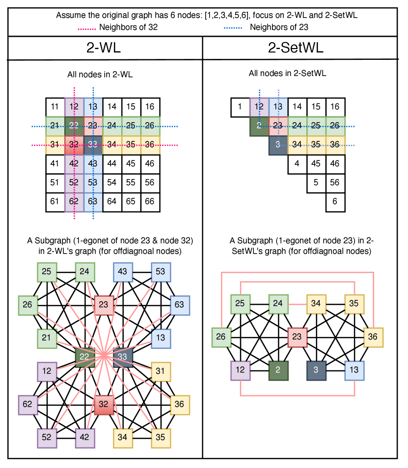
A.1 Visualization Supergraph Connection of 2-SetWL
A.2 Bijective -Pebble Game for -WL
The pebble game characterization of k-FWL appeared in [11]. We use the pebble game defined in [28] for k-WL. Let be graphs and be -tuple. Then the bijective -pebble game () is defined as the follows. The game is played by two players Player I and Player II. The game proceeds in rounds starting from initial position and continues to new position as long as after rounds defines an isomorphism between and . If the game has not ended after rounds, Player II wins the -step (), otherwise Player I wins.
The -th round is played as follows.
-
1.
Player I picks up the -th pair of pebbles with .
-
2.
Player II chooses bijection .
-
3.
Player I chooses .
-
4.
The new position is (, ). If and are still isomorphic, the game continues. Otherwise, the game ends and Player II loses.
The game () has the same expressivity as -WL in distinguishing () and ().
Theorem 9.
-WL cannot distinguish () and () at step , i.e. , if and only if Player II has a winning strategy for -step ().
There is an extension of the pebble game, (), without specifying the starting position. Specifically, at the beginning of the game, Player II is first asked to provide a bijection Then Player I chooses . Then Player I and Player II start to play ().
Theorem 10.
-WL cannot distinguish G and at step , i.e. , if and only if Player II has a winning strategy for -step (.
A.3 Doubly Bijective -Pebble Game for -MultisetWL
Let be graphs and be -multisets. We adapt the game for -MultisetWL and call it doubly bijective -pebble game, i.e. . A similar version of the pebble game for -MultisetWL was suggested by Grohe in [27].
The is defined as the follows. The game starts at the position ().
Let the current position be . The -th round is played as follows.
-
1.
Player II chooses a bijection
-
2.
Player I chooses the
-
3.
Player II chooses bijection
-
4.
Player I chooses
-
5.
The new position is and the game continues, if and are isomorphic. Otherwise the game ends and Player II loses.
To extend the game to the setting of no starting position, we define the corresponding game . Simliar to , at the beginning Player II is asked to pick up a bijection . Then Player I picks up a and the game starts.
Theorem 3.
-MultisetWL has the same expressivity as the doubly bijective -pebble game.
Proof.
Specifically, given graph with -multiset and graph with -multiset , we are going to prove that Player II has a winning strategy for -step game .
We now prove it by induction on . When , it’s obvious that the statement is correct, as is equivalent to and being isomorphic, which implies that Player II can start the game without losing. Now assume that for the statement is correct. For step , let’s first prove left right.
. By Eq.(3) we know this is equivalent to
(1)
(2) ,
, .
Now let’s start the game at position (). By (2) we know that there exist a satisfying (2). Then at the first round, we as Player II pick the as the bijection. Next Player I will choose a . According to (2), for the and we have . This implies that there exists a bijection such that . Hence let Player II pick the . Now player I will choose a . Then implies , hence and are isomorphic. So the game doesn’t end. At the next round, the game starts at the position , and we know . By the inductive hypothesis, Player II has a strategy to play DBPk at the new position for rounds. Hence Player II has a winning strategy to play DBPk at original position () for rounds.
Next we prove right left by showing that Player I has a winning strategy for -step game .
implies:
(1)
or
(2) for any bijection , , such that
If (1) holds, then by induction we know that Player I has a winning strategy within -steps hence Player I also has a winning strategy within steps. If (2) holds, then at the first round after Player II picks up a bijection , Player I can choose the specific with . Then no matter which bijection Player II chooses, Player I can always choose a such that . Then by induction, Player I has a winning strategy within -steps for the DBPk starts at position . Hence even if Player I doesn’t win in the first round, he/she can still win in rounds.
Combining both sides we know that the equivalence between -step DBPk and -step -MultisetWL holds for any and any -multisets.
∎
Theorem 11.
-MultisetWL cannot distinguish G and at step , i.e. , if and only if Player II has a winning strategy for -step (.
Proof.
The proof is strict forward with using the proof inside Theorem 3. We just need to show that the pooling of all -multisets representations is equivalent to Player II finding a bijection at the first step of the game. We omit that given its simplicity. ∎
A.4 Proofs of Theorems
A.4.1 Bound of Summation of Binomial Coefficients
Derivation of:
| (15) |
Proof.
| (16) | ||||
| (17) | ||||
| (18) | ||||
| (19) |
∎
A.4.2 Proof of Theorem 1
Theorem 1.
Let and . For all and all graphs : -MultisetWL is upper bounded by -WL in distinguishing multisets and at -th iteration, i.e. .
Proof.
By induction on . It’s obvious that when the above statement hold, as both side are equivalent to and being isomorphic to each other. Assume the above statement is true. For case, by definition the left side is equivalent to . Let be the ordered version of following canonical ordering over , then there exists a bijective mapping between and , such that , where . By [11]’s Theorem 5.2, for any , is equivalent to that player II has a winner strategy for -step pebble game with initial configuration and (please refer to [11] for the description of pebble game). Notice that applying any permutation to the pebble game’s initial configuration won’t change having winner strategy for player II, hence we know that , . Now applying Eq.(1), we know that (1) , and (2), = . We rewrite (2) as, , , , . As (1) and (2) hold for any , now applying induction hypothesis to both (1) and (2), we can get (a) , and (b) , , , , where is the index mapping function corresponding to . Now we rewrite (b) as , , . Combining (a) and (b), using Eq.(3) we can get . Thus for any the above statement is correct. ∎
A.4.3 Proof of Theorem 2
CFI Graphs and Their Properties
Cai, Furer and Immerman [11] designed a construction of a series of pairs of graphs CFI(k) such that for any , -WL cannot distinguish the pair of graphs CFI. We will use the CFI graph construction to prove the theorem. Here we use a variant of CFI construction that is proposed in Grohe et al.’s work [28]. Let he a complete graph with nodes. We first construct an enlarged graph from the base graph by mapping each node and edge to a group of vertices and connecting all groups of vertices following certain rules. Notice that we use node for base graph and use vertex for the enlarged graph for a distinction. Let denotes the edge connecting node and node . For a node , let denotes the set of all adjacent edges of in the graph .
For every node , we map node to a group of vertices with size . For every edge , the construction maps to two vertices . Hence there are number of vertices in the enlarged graph with . Let and .
Now edges inside are defined as follows
| (20) | ||||
| (21) |
What’s more, we also color the vertices such that all vertices inside have color for every and all vertices inside have color for every . See Figure.4 top right for the visualization of transforming from base graph to with .

There are several important properties about the automorphisms of . Let be an automorphism, then
-
1.
and for all and .
-
2.
For every subset , there is exactly one automorphism that flips precisely all edges in F, i.e. and if and only if . More specifically,
-
•
-
•
-
•
,
where
-
•
Proof.
These properties are not hard to prove. First for property 1, it is true based on the coloring rules of vertices in . Now for the second property. As flips precisely all edges in , we have and . Now let , we need to figure out ’s formulation. Let’s focus on node without losing generality, and we can partition the set to two parts: and . Then for any , we know that . Let denote that and are connected in . Then , . And similarly we have , . Hence , . This implies that . Following the same logic we can also get , , which is equivalent to , which further implies that as . Then combining both side we know that . Hence we get . ∎
In the proof we can also know another important property. That is is constant for any input .
Now we are ready to construct variants of graphs that are not isomorphic from the enlarged graph . Now let T be a subset of . Now we define an induced subgraph of the enlarged graph . Specifically, we define the new node group as follows
| (22) |
Then the induced subgraph is defined as . In Figure 4 we show in bottom left (labeled with ) and in the bottom right (labeled with ).
Lemma 1.
For all , if and only if . And if they are isomorphic, one isomorphism between and is with , where denotes the set of all edges .
Notice that is an automorphism for , but with restricting its domain to it becomes the isomorphism between and .
The proof of the lemma can be found in [11] and [28]. With this lemma we know that and are not isomorphic. In next part we show that and cannot be distinguished by -WL but can be distinguished by -MultisetWL, thus proving Theorem 2.
Main Proof
Theorem 2.
-MultisetWL is no less powerful than (-)-WL in distinguishing graphs: for there is a pair of graphs that can be distinguished by -MultisetWL but not by (-)-WL.
Proof.
To prove the theorem, we show that for any , and , defined previously, are two nonisomorphic graphs that can be distinguished by -MultisetWL but not by -WL. It’s well known that these two graphs cannot be distinguished by -WL, and one can refer to Theorem 5.17 in [28] for its proof. Now to prove these two graphs can be distinguished by -MultisetWL, using Theorem 11 we know it’s equivalent to show that Player I has a winning strategy for the doubly bijective -pebble game .
At the start of the pebble game , Player II is asked to provide a bijection between all -multisets of to all -multisets of . For any bijection the Player II chosen, the Player I can pickup , with corresponding position . Notice that for a position , the position is called consistent if there exists a , such that . One can show that Player I can easily win the game after one additional step if the current position is not consistent, even if and are isomorphic [28].
We claim that for any -multiset the position cannot be consistent, and thus Player II loses after the first round. Assume that there exists a subset , such that . By property 1 of automorphisms of we have that , and since contains exactly one vertex of each color, it also holds that . It follows from property 2 that . Based on the definition of , we know that , and thus flips an odd number of neighbors of , i.e. . Similarly, we have that and , hence . It follows from a simple handshake argument that there exists an such that
which is a contradiction. Hence Player I has a winning strategy for .
∎
A.4.4 Proof of Theorem 3
See Appendix.A.3.
A.4.5 Proof of Theorem 4
Theorem 4.
Let , then and all graphs : .
Proof.
Notation: Let transform a multiset to set by removing repeats, and let return a tuple with the number of repeats for each distinct element in a multiset. Let be the inverse mapping such that .
Define . Let .
Lemma 2.
, , , .
When , by the definition of , the statement is true. Now hypothesize that the statement is true for case. For case, the left side implies that existing a with and a with , such that . And for a mapping , we have , .
For a specific , define and .
By Eq.(3):
(1) ;
(2) ,
, .
As , we can change (2) by choosing as . Hence we update it as:
(2) ,
And (2) can be split into two parts:
(2) , and
Combining the Lemma.2 and induction hypothesis, also knowing that and , we get:
(a) ;
(b) , , this is derived with picking with , such that only has 1 and only has 1 .
(c) , , this is derived with picking with .
(d) , , this is derived with picking with , such that only has 1 and only has 1 .
Now combining (a) (b) (c) (d) and using Eq.(5), we can get that , and we proved the statement.
∎
A.4.6 Proof of Theorem 5
Theorem 5.
Let , then and all graphs :
-
(1)
when , if cannot be distinguished by -SetWL, they cannot be distinguished by -SetWL
-
(2)
when , , if cannot be distinguished by -SetWL, they cannot be distinguished by -SetWL
Proof.
We will prove (2) first, and the proof for (1) follows the same argument. To help understand, we present the formulation for -SetWL first.
| (23) | |||
| (24) | |||
| (25) |
Lemma 3.
For , for any , for any and with nodes inside, .
Proof of Lemma.3:
Proof.
We prove it by induction. As the color initialization stage of -SetWL and -SetWL are the same, when the statement of the Lemma is correct. Assume it holds correct for . When , implies:
(1) =
(2) =
(3)
=
(4)
=
(1) + induction hypothesis (a) =
(2) has two situations: and . For the first situation, and , a bijective mapping between and such that , = and by induction = , hence = . For the second situation, elements while , then clearly (b) = (both are empty multisets).
(3) follows the same argument step in (2)’s first situation, with induction hypothesis we can get (c)
=
(4) implies that a mapping between and such that for any , = . Using the same argument in (2) and induction hypothesis, this implies that for any , = . Hence we get (d)
= .
Combining (a) (b) (c) (d) we get . ∎
With Lemma.3 we are ready to prove (2) in Theorem 3. When two graphs and cannot be distinguished by -SetWL, we have = . When and have different (number of nodes) and (number of components of its induced subgraph), their color cannot be the same (as already be different). Hence = is equivalent to , = . With Lemma.3 we can get that , = . Hence two graphs and cannot be distinguished by -SetWL.
∎
A.4.7 Proof of Theorem 6
Theorem 6.
When () BaseGNN can distinguish any non-isomorhpic graphs with at most nodes, () all MLPs have sufficient depth and width, and () POOL is an injective function, then for any , -layer -SetGNN is as expressive as -SetWL at the -th iteration.
Proof.
For any , let denotes the color of at -iteration -SetWL and denotes the embedding of at -th layer -SetGNN. We prove the above theorem by showing that = = . We remove the subscript when possible without introducing confusion.
For easier reference, recall the updating formulation for -iteration -SetWL is
| (26) | ||||
| (27) | ||||
| (28) |
And the updating formulation for -SetGNN is
| (29) | ||||
| (30) | ||||
| (31) |
At , given powerful enough BaseGNN with condition (i) in the theorem, = and are isomorphic = .
Now assume for iterations the claim = = holds (for any and ). We prove it holds for iteration. We first prove the forward direction. = imples that
(1) =
(2) =
(3)
=
(4)
=
(1) and (3) can be directly transformed to relationship between using the inductive hypothesis. Formally, we have
(a) = and
(c)
=
(2) and (4) need one additional process. Notice that (2) is equivalent to and by inductive hypothesis we know . As the formulation Eq.(29) applies a MLP with summation, which is permutation invariant to ordering, to the multiset , the same multiset leads to the same output. Hence we know
(b) = .
For (4) we know that there is a bijective mapping between and such that . Then using the same argument as (2) =>(b) we can get for any , which is equivalent to
(d)
= .
Combining (a)(b)(c)(d) and using the permutation invariant property of MLP with summation, we can derive that = .
Now for the backward direction. We first characterize the property of MLP with summation from DeepSet [64] and GIN [61]’s Lemma 5.
Lemma 4 (Lemma 5 of [61]).
Assume is countable. There exists a function so that is unique for each multiset of bounded size.
Using this Lemma, we know that given enough depth and width of a MLP, there exist a MLP that or in other words two multisets and are equivalent. Now by = and using the Eq.(31), we know there exists MLPs inside Eq.(29) and Eq.(31), such that
(1) =
(2) =
(3)
=
(4)
=
Where (3) and (4) are derived using the provided lemma. Hence following the same argument as the forward process, we can prove that = .
Combining the forward and backward direction, we have = = . Hence by induction we proved for any step and any , the above statement is true. This shows that -SetGNN and -SetWL have same expressivity.
∎
A.4.8 Proof of Theorem 7
Theorem 7.
For any , the -layer -SetGNN∗ is more expressive than the -layer -SetGNN. As , -SetGNN is as expressive as -SetGNN∗.
Proof.
We first prove that -layer -SetGNN∗ is more expressive than -layer -SetGNN, by showing that if a -set has the same representation to another -set in -layer -SetGNN∗, then they also have the same representation in -layer -SetGNN. Let be the representation inside -SetGNN∗, and be the representation inside -SetGNN.
To simplify the proof, we first simplify the formulations of -SetGNN∗ Eq.13 and Eq.14 by removing unnecessary super and under script of MLP without introducing ambiguity. We then add another superscript to embeddings to indicate which step inside the one-layer bidirectional propagation. Notice that for one-layer bidirectional propagation, there are intermediate sequential steps. The proof assumes that all MLPs are injective. We rewrite Eq.13 and Eq.14 as follows
| (32) | |||
| (33) |
Where we have boundary case with and . represents that the representation is calculated at step for layer.
We prove the theorem by induction on . Specifically, we want to prove that for any , , , and . The base case is easy to verify as the definition of initialization step is the same.
Now assume that for we have for any , , , and . We first prove that for , .
First, Eq.32 can be rewrite as
| (34) | |||
| (35) |
Then . Hence we can find a bijective mapping between and such that . Then by inductive hyphothesis, for all . This implies that or equivalently .
Now we can assume that for we have for any , , , and for . We prove that for , .
1) or equivalently
2) =
Also by Eq.32 we know that implies
3) .
Combining with 2) and 3) we know
4) =
Now using our inductive hypothesis, we can transform 1) 2) 3) 4) by replace with . Then based on the equation in 11, we know .
Combining the two proved inductive hypothesis and applying them alternately, we know that for any , , , and . Hence -layer -SetGNN∗ is more expressive than -layer -SetGNN.
Now let’s considering to infinity. Then all representations will become stable with and . Notice that for a single set , the information used from its neighbors are the same in both -SetGNN and -SetGNN∗. Hence the equilibrium equations for set should be the same in both -SetGNN and -SetGNN∗. Then they will have the same stable representations at the end.
∎
A.4.9 Proof of Theorem 8
Theorem 8.
Let be a graph with connected components , and be a graph also with connected components , then and are isomorphic if and only if , s.t. , and are isomorphic.
Proof.
Right Left. Let be one isomorphism from to for . Then we can create a new mapping , such that for any , it first locates which component inside, for example , then apply to . Clearly is a isomorphism between and , hence and are isomorphic.
Left Right. and are isomorphic, then there exists an isomorphism from to . Now for a specific component in , maps to a nodes set inside , and name it as . For , and there is not edges between and otherwise there must be an corresponding edge (apply ) between and which is impossible. Hence are disconnected subgraphs. As also preserves connections, for any , and are isomorphic. Hence we proved the right side.
∎
A.4.10 Conjecture that k-MWL is equvialent to k-WL
Proof of
Proof.
We first take a closer
look at the condition of . By Eq.(3) we know this is equivalent to
(1) and (2) = . (2) can be rewrite as = , which is equivalent to (3) , , .
Define . Let .
Lemma 5.
, if and only if .
Notice that this Lemma is conjectured to be true. This needs additional proof.
Lemma 6.
Proof of Lemma.6: We prove it by induction on . When , contains all isomorphisms between and , hence the right side is correct. Assume the statement is correct for . For case, the left side implies (1) and (2), , , , , . By induction hypothesis, (1) and imply (a) ; (2) and , imply (b) , , , which can be rewritten as , = . Now applying Eq.(1) with (a) and (b), we can derive that , . Hence the statement is correct for any .
A.5 Algorithm of extracting sets and constructing the super-graph of -SetWL
Here we present the algorithm of constructing supernodes sets from supernodes sets, and constructing the bipartite graph between sets and sets. Notice the algorithm we presented is just the pseudo code and we use for-loops to help presentation. The algorithm can easily be parallelized (removing for-loops) with using matrix operations.
To get the full supergraph , we need to apply Algorithm.1 times sequentially.
A.6 Algorithm of connecting supernodes to their connected components
In Sec.4.3 we proved that for a supernode with multi-component induced subgraph (call it multi-component supernode), the color initialization can be greatly sped up given knowing its each component’s corresponding supernode. Hence we need to build the bipartite graph (call it components graph) between single-component supernodes and multi-component supernodes. We present the algorithm of constructing these kind of connections sequentially. That is, given knowing the connections between single-component supernodes and all multi-component supernodes with number of nodes, to build the connections between single-component supernodes and all multi-component supernodes with number of nodes. To build the full bipartite graph for sets, we need to conduct the algorithm times sequentially.
For the clear of presentation we use for-loops inside Algorithm.2, while in practice we use matrix operations to eliminate for-loops.
A.7 Dataset Details
| Dataset | Task | # Cls./Tasks | # Graphs | Avg. # Nodes | Avg. # Edges |
| EXP [1] | Distinguish 1-WL failed graphs | 2 | 1200 | 44.4 | 110.2 |
| SR25 [6] | Distinguish 3-WL failed graphs | 15 | 15 | 25 | 300 |
| CountingSub. [15] | Regress num. of substructures | 4 | 1500 / 1000 / 2500 | 18.8 | 62.6 |
| GraphProp. [17] | Regress global graph properties | 3 | 5120 / 640 / 1280 | 19.5 | 101.1 |
| ZINC-12K [19] | Regress molecular property | 1 | 10000 / 1000 / 1000 | 23.1 | 49.8 |
| QM9 [59] | Regress molecular properties | 19222We use the version of the dataset from PyG [20], and it contains 19 tasks. | 130831 | 18.0 | 37.3 |
A.8 Experimental Setup
Due to limited time and resource, we highly restrict the hyperparameters and fix most of hyperparameters the same across all models and baselines to ensure a fair comparison. This means the performance of -SetGNN∗ reported in the paper is not the best performance given that we didn’t tune much hyperparameters. Nevertheless the performance still reflects the theory and designs proposed in the paper, and we postpone studying the SOTA performance of -SetGNN∗ to future work. To be clear, we fix batch size to 128, the hidden size to 128, the number of layers of Base GNN to 4, and the number of layers of -SetGNN∗ (the number of iterations of -SetWL) to be 2 (we will do ablation study over it later). This hyperparameters configuration is used for all datasets. We have run the baseline GINE over many datasets, and we tune the number of layers from [4,6] and keep other hyperparameters the same as -SetGNN∗. For all other baselines, we took the performance reported in [68].
For all datasets except QM9, we follow the same configuration used in [68]. For QM9, we use the dataset from PyG and conduct regression over all 19 targets simultaneously. To balance the scale of each target, we preprocess the dataset by standardizing every target to a Gaussian distribution with mean 0 and standard derivation 1. The dataset is randomly split with ratio 80%/10%/10% to train/validation/test sets (with a fixed random state so that all runs and models use the same split). For every graph in QM9, it contains 3d positional coordinates for all nodes, and we use them to augment edge features by using the absolute difference between the coordinates of two nodes on an edge for all models. Notice that our goal is not to achieve SOTA performance on QM9 but mainly to verify our theory and effectiveness of designs.
We use Batch Normalization and ReLU activation in all models. We use Adam optimizer with learning rate 0.001 in all experiments for optimization. We repeat all experiments three times (for random initialization) to calculate mean and standard derivation. All experiments are conducted on V100 and RTX-A6000 GPUs.
A.9 Graph Property Dataset Results
| Regressing Graph Properties ((MSE)) | |||||||
| Is Connected | Diameter | Radius | |||||
| k | c | Train | Test | Train | Test | Train | Test |
| 2 | 1 | -4.2266 ± 0.1222 | -2.9577 ± 0.1295 | -4.0347 ± 0.0468 | -3.6322 ± 0.0458 | -4.4690 ± 0.0348 | -4.9436 ± 0.0277 |
| 3 | 1 | -4.2360 ± 0.1854 | -3.4631 ± 0.6392 | -4.0228 ± 0.1256 | -3.7885 ± 0.0589 | -4.4762 ± 0.1176 | -5.0245 ± 0.0881 |
| 4 | 1 | -4.7776 ± 0.0386 | -4.9941 ± 0.0913 | -4.1396 ± 0.0442 | -4.0122 ± 0.0071 | -4.2837 ± 0.5880 | -4.1528 ± 0.9383 |
| 2 | 2 | -4.6623 ± 0.3170 | -4.7848 ± 0.3150 | -4.0802 ± 0.1654 | -3.8962 ± 0.0124 | -4.5362 ± 0.2012 | -5.1603 ± 0.0610 |
| 3 | 2 | -4.2601 ± 0.3192 | -4.4547 ± 1.1715 | -4.3235 ± 0.3050 | -3.9905 ± 0.0799 | -4.6766 ± 0.1797 | -4.9836 ± 0.0658 |
| 4 | 2 | -4.8489 ± 0.1354 | -5.4667 ± 0.2125 | -4.5033 ± 0.1610 | -3.9495 ± 0.3202 | -4.4130 ± 0.2686 | -4.1432 ± 0.4405 |
A.10 Ablation Study over Number of Layers
| L | 2 | 4 | 6 | ||||
| k | c | Train | Test | Train | Test | Train | Test |
| 2 | 1 | 0.1381 ± 0.0240 | 0.2345 ± 0.0131 | 0.1135 ± 0.0418 | 0.1921 ± 0.0133 | 0.0712 ± 0.0015 | 0.1729 ± 0.0134 |
| 3 | 1 | 0.1172 ± 0.0063 | 0.2252 ± 0.0030 | 0.0792 ± 0.0190 | 0.1657 ± 0.0035 | 0.0692 ± 0.0118 | 0.1679 ± 0.0061 |
| 4 | 1 | 0.0693 ± 0.0111 | 0.1636 ± 0.0052 | 0.0700 ± 0.0085 | 0.1566 ± 0.0101 | 0.0768 ± 0.0116 | 0.1572 ± 0.0051 |
A.11 Computational Footprint on QM9


A.12 Discussion of k-Bipartite Message Passing

Interestingly, the k-bipartite bidirectional message passing is very general and its modification covers many well known GNNs. Considering only using 1-sets and 2-sets with single connected components (the red frame inside Figure 6), and initializing their embeddings with their original nodes and edges representations, then it covers the follows
- •
- •
- •