A Polymer Chain with Dipolar Active Forces in Connection to Spatial Organization of Chromatin
Abstract
A living cell is an active environment where the organization and dynamics of chromatin are affected by different forms of activity. Optical experiments report that loci show subdiffusive dynamics and the chromatin fiber is seen to be coherent over micrometer-scale regions. Using a bead-spring polymer chain with dipolar active forces, we study how the subdiffusive motion of the loci generate large-scale coherent motion of the chromatin. We show that in the presence of extensile (contractile) activity, the dynamics of loci grows faster (slower) and the spatial correlation length increases (decreases) compared to the case with no dipolar forces. Hence, both the dipolar active forces modify the elasticity of the chain. Interestingly in our model, the dynamics and organization of such dipolar active chains largely differ from the passive chain with renormalized elasticity.
I Introduction
Active systems are inherently out of equilibrium [1]. It consumes energy perpetually from the environment which prevents relaxation into a thermal equilibrium state and exhibits a wide spectrum of novel steady-state behaviours such as the activity-driven phase separation [2] or large-scale collective motion [3]. Even inside the living cells, active systems have constituents that adapt in noisy environments and generate forces for uni-directional transport and spatial organization. Biopolymers are an integral part of living cells, and their conformational and dynamical properties are significantly affected by the active processes [4, 5, 6, 7, 8, 9, 10, 11]. For example, the microtubule and F-actin filaments of the cytoskeleton are driven forward by the myosin and kinesin families of motor proteins [12, 13]. Another biopolymer inside the nucleus is chromosomal DNA [14, 15, 16] and it serves as a platform for number of biological processes such as Chromatin remodelling [17], transcription [18] and DNA repair [19]. Their spatial organization dramatically varies along with the different phases of the cell cycle, which seem to be driven by processes that consume ATP [20, 21]. However, the exact procedure of energy consumption on the chromatin remains unclear and this is the primary interest of the present study.
Interphase chromatin are organized into transcriptionally active and inactive regions. Transcriptionally active regions, referred to as euchromatin, are loosely packed, whereas transcriptionally inactive regions, called heterochromatin, are tightly packed [22], [23]. In a recent study, transcriptionally active regions are characterized by an effective temperature in which a Brownian-like random force is acting on chromosomes in addition to thermal noise [24, 25]. Weber argued that random motions of chromatin loci in are driven by the ATP-dependent fluctuations which behave like thermal fluctuations but with a greater magnitude [26]. However, Liu showed that the enhanced thermal like fluctuations due to activity randomize the global structure of chromatin chain more efficiently as compared to the thermal noise and shorten the spatial correlation at a sufficiently large time [27]. On contrary, Zidovska demonstrated two types of chromatin motion experimentally: a fast local motion previously observed by tracking the motion of chromosomal loci and a slower large-scale motion in which collective motions of chromatin are seen to be coherent beyond the boundaries of chromosome territories, over micrometer-scale regions and seconds [28]. To explain the correlated motions of chromatin, Saintillan constructed a flexible polymer model with long-range hydrodynamic interactions that is driven by active force dipoles [29]. In their model, they obtained strong correlated motion for extensile activity, but not in the cases of passive and contractile activity [30]. In another study, Liu modelled the chromatin as active flexible polymer subjected to extensile and contractile monopoles [31]. They showed that both the extensile and contractile monopoles generate correlated motion without the hydrodynamic interactions and the contractile system exhibits larger displacements than the extensile one. Other theoretical models of active polymers have also been proposed in connection to chromosomal dynamics. Some of these models have focused on semiflexible [32] or flexible polymer [33] chains subject to correlated noise or an active force parallel to the backbone of the chain [34]. Hence, the dynamics is superdiffusive in such models. A recent study in mouse embryonic stem cells showed that differentiated chromatin moves by an apparent free diffusion, while the undifferentiated one behaves superdiffusively [35].
To understand how the large-scale correlated chromatin dynamics emerges from the local subdiffusive motion, we construct a model for chromatin as a long semiflexible polymer with excluded volume interactions and dipolar extensile and contractile activities. We do not include hydrodynamic interactions in this study. We show that both the extensile and contractile active forces modify the elasticity of the chain, but leave the subdiffusive nature of the loci dynamics unchanged. We compare our results for dipolar activity to thermal system with renormalized elasticity and find that dipolar active forces create larger expansion or compaction of the chain as compared to thermal system with renormalized elasticity. Hence, dipolar active forces can not be thought of as a thermal system with renormalized elasticity.
II Model
We consider a bead-spring polymer chain composed of monomers of radius in a three-dimensional space. We implement the following overdamped Langevin equation to simulate the dynamics of all the monomers of our system with the position (t) at time :
| (1) |
where is the friction coefficient which is related to the thermal Gaussian noise through
| (2) |
The total potential energy, is composed of a bond contribution between neighbouring beads
| (3) |
a bending energy
| (4) |
and an excluded volume interaction modelled with Weeks-Chandler-Andersen (WCA) potential [36]:
| (5) |
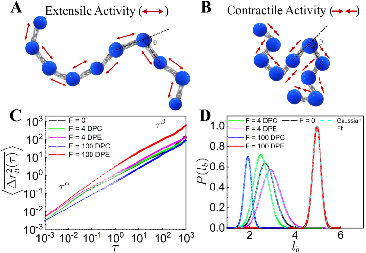
where is the vector between the position of the beads and , is the force constant, is the equilibrium bond distance, , is the bending modulus, is the separation between a pair of monomers in the medium, is the strength of the interaction, and determines the effective interaction diameter. Without the force, , the model matches with the well-known worm-like chain model for semi-flexible polymers. Here denotes the dipolar active forces on each bead that pushes simultaneously two neighbouring beads towards (contractile) or away (extensile) from each other along the unit bond vector for all the time with constant magnitude (Fig. 1 (A, B)). For the extensile case, the force and are exerted on the and monomers respectively. Thus, the extensile force on the monomer, . Similarly, for the contractile force, . This is where our model differs from the existing models where activity is introduced by putting the beads at a higher temperature [24, 25]. The dipolar extensile or contractile active forces in our model can be derived from a potential or . In the works by Prathyusha [37] or Isele-Holder [38], the magnitude of the active force is constant and the direction is acting along the unit bond vector of the polymer. The active forces modeled in these works can also be generated from a potential, but not dipolar in nature. Therefore, the composite system made of polymer and the activity behave like a thermal system and the total force on the composite system will be conservative. We do not incorporate any binding rates of the active force [32, 33] in the model which might modify the magnitude of the active force by a factor. In our simulation, we consider , and as the unit of length, energy and time scales. The parameters used for the simulation are , , , . All the production simulations are carried out for steps where the integration time step is considered to be . The simulations are carried out using LAMMPS [39], a freely available open-source molecular dynamics package. For a given set of parameters, we generate independent trajectories of the polymer.
III Results
III.1 Mean Square Displacement
To quantify the effect of dipolar extensile (DPE) and dipolar contractile (DPC) activities on the dynamics of the individual monomers, we first focus on the time-and-ensemble averaged mean squared displacement (MSD) of the tagged monomer in the reference frame of the polymer’s center of mass
(COM), as a function of lag time . The time-averaged MSD of -th monomer is defined as from the time series where is the total run time. The time-and-ensemble-averaged MSD is obtained by summing over all the monomers as: where is the number of monomers. For small DPE and DPC activities , the dynamics of the tagged monomer is subdiffusive (see supplementary Table S1) and we do not see any significant enhancement in as compared to the passive case as evident in Fig. 1C. But, for very high DPE and DPC activities , we observe a clear difference in , while the subdiffusive dynamics of the monomer remains unaltered. In comparison to the passive case, the dynamics of the individual monomer is enhanced for high DPE force and suppressed for high DPC force respectively (Fig. 1C). However, the dipolar activity leaves the dynamical behavior of the COM unchanged (see supplementary Fig. S1), suggesting that the effective temperature as introduced in earlier studies of chromatin [24, 32], is not a good descriptor for dipolar activity. Hence, the responses of the COM and individual monomer in the presence of dipolar activity suggest that the dipolar forces modify the stretching of the chain which essentially enhances or reduces the local space explored by the tagged monomer for the DPE or DPC forces respectively, but not the diffusive or subdiffusive nature of the displacements.
III.2 Distribution of Bond Lengths
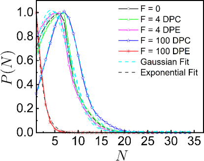
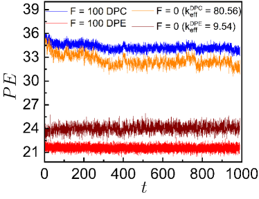
To further quantify the effects of the DPE and DPC active forces on the loci mobilities, we investigate the probability distribution, of the bond length, of the chain. We calculate for different bonds at each time-step of every simulation after the system reaches the steady-state where is the number of monomers. Then a single trajectory is created by joining different individual trajectories. This single trajectory is binned to construct a histogram from which the ensemble averaged probability distribution is computed. Here values follow Gaussian distributions (Fig. 1D). For smaller DPC and DPE activities, values appear to be qualitatively similar to of the passive system. But, values for high DPE and DPC forces show well-separated peaks (Fig. 1D). For large DPE force, the peak of shifts towards a higher value of which accounts for the enhancement of stretching of the polymer chain. For large contractile force, is sharply peaked at lower value of and the deviation of the peak value of from the passive case is small as compared to the deviation for the DPE force. This small deviation for the contractile force is presumably due to the self-avoidance of the beads. The potential energy (PE) per particle increases more for the DPC forces than for the DPE forces (see supplementary Fig. S2A) as the effect of self-avoidance translates to an increasing potential energy barrier for the contractile forces. On the other hand, the mean square fluctuation of the velocity , per particle increases more for the DPE forces than for the DPC forces (see supplementary Fig. S2B) as the DPE forces show larger displacements than the DPC forces. Additionally, the probability distribution, of the radius of gyration of the chain and the distribution, of number of monomers, in a spherical probe volume indicate that DPE (or DPC) forces promote larger (or smaller) displacements of the system than the passive one (see supplementary Sec. III & IV and Fig. S3 & S4).
III.3 Spatio-temporal Correlation
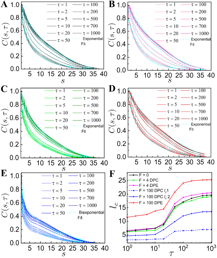
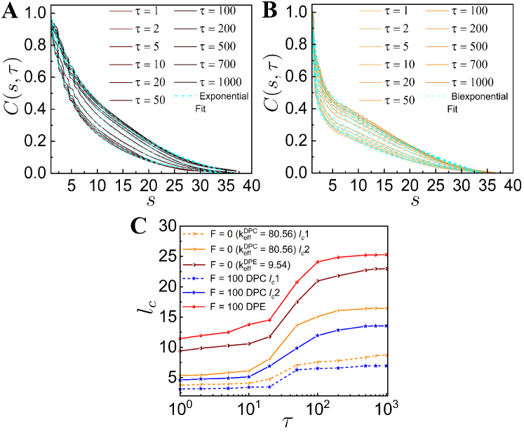
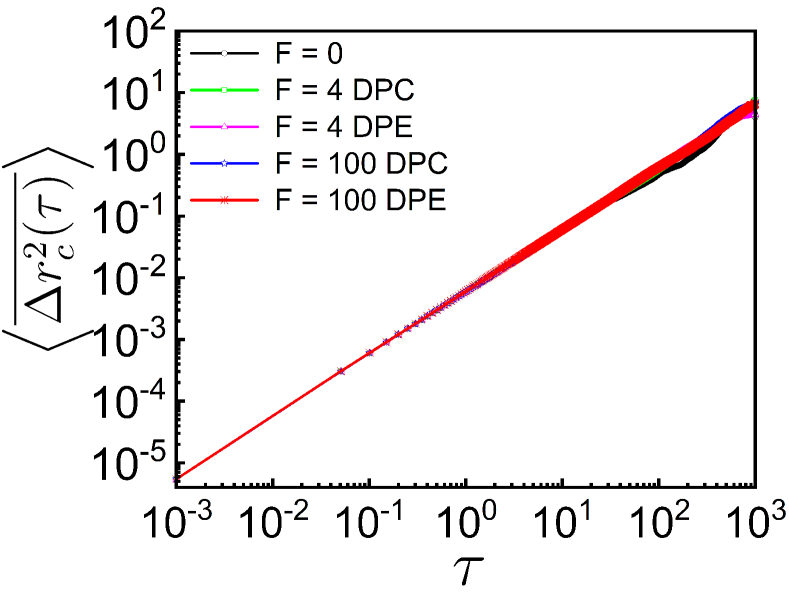
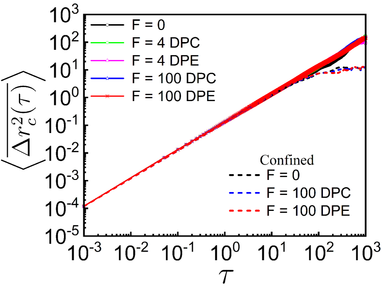
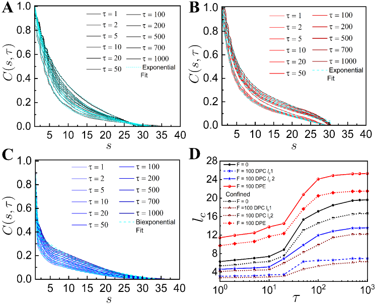
To study the spatio-temporal dynamics of our chromatin model, we calculate the spatial correlation function, as a function of spatial distance between two loci for different values of the lag time [28]. The normalized spatial correlation between -th and -th loci over the time interval is evaluated as where is an average over and over different ensembles. As increases, values show slower spatial decay both in the case of with and without the active dipolar forces (Fig. 2). For passive and smaller DPC and DPE activities, values decay exponentially (Fig. 2 (A-C)). The corresponding correlation lengths, increase monotonically with and eventually saturated at large (Fig. 2F), which is consistent with the experimental observation [40]. shows similar exponentially decaying correlation with for higher DPE force (Fig. 2D). For large DPC force, we fit with an bi-exponentially decaying function where and represent the correlation lengths for the initial faster and subsequent slower decay respectively (Fig. 2 (E, F)). The correlation length of extensile active systems is greater than the same for the contractile active systems. This suggests that the motion of extensile active chain has long-ranged spatial coherence than the contractile active chain.
III.4 Distribution of Bending Fluctuations
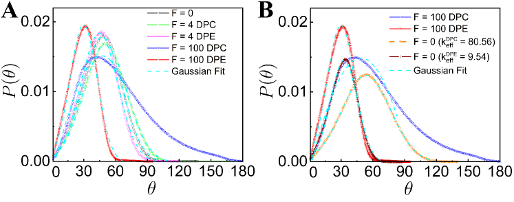
Other than , we look at the normalized distribution of local curvatures to characterize the internal structure more quantitatively, where is the bond angle between the bond vectors. Fig. 3A shows that for small DPC and DPE activities, values are Gaussian and nicely collapse on of the passive system. However, for large DPC and DPE systems, values display a clear difference from passive system. for DPE chain with higher activity exhibits a peak at smaller bond angle and the width of becomes narrower as compared to that of the DPC chain with higher activity (Fig. 3A). Fig. 3B is discussed in the latter part of the manuscript. Narrowed distribution of with peak value at small bond angle for high DPE force implies effectively higher bending rigidity as compared to that of passive chain. This again confirms that extensile activity induces long-ranged spatial correlations compared to contractile activity.
IV Comparison with the Effective Equilibrium Model
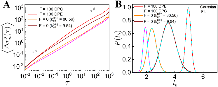
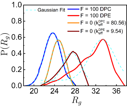
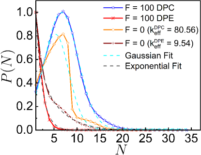
In our model of dipolar activity, DPE and DPC forces are working on every bead along the unit bond vector with constant magnitude, . Another option is to introduce thermal extensile or contractile forces acting along the bond vector. The thermal extensile forces on the th bead due to th and th beads become and respectively where is the average bond length. The net force on th bead, becomes in the continuum limit. Thus, the effective spring constant is reduced by for the thermal extensile case. Similarly, for the thermal contractile case, is enhanced by . We calculate from the distribution of (Fig. 1D) for both the extensile and contractile forces. Next, we simulate Eq. (1) with and modified spring constants, and respectively. For , the spring constant, of the thermal chain is modified to for extensile chain with and to for contractile chain with . We compare the results, (Fig. 4A), (Fig. 4B) and (Fig. 5) of our model of dipolar activity to thermal chain with these modified spring constants and . We find that the thermal chain with is less stretched than the chain with active dipolar extensile force . Similarly, the thermal chain with is less compressed than the chain with active dipolar contractile force . In a semiflexible polymer, stretching and bending coefficients are not independent of each other [32]. Hence, if the stretching coefficient is modified, it also modifies the bending coefficient as evident in Fig. 3B. Large DPE (or DPC) activity strongly increases (or decreases) the probability of long straightened segments as compared to thermal chain with renormalized spring constants, and . The behavior of steady state and PE (see supplementary Fig. S5), (see supplementary Fig. S6) and, (see supplementary Fig. S7) for both the dipolar activities and the thermal chain with and are given in the Supporting Material and we observe similar trends, DPE (or DPC) active forces promote larger (or smaller) displacements of the system than the thermal one with (or ). The stretching (or compression) of the thermal chain with lower (or higher) spring constants as compared to the chain with large dipolar extensile (or contractile) activities arise because the magnitude of the dipolar active force is constant whereas the magnitude of the spring force is fluctuating. This leads us to propose that the extensile (or contractile) dipolar active system can not be mapped to a thermal system with larger (or lower) bending modulus and longer (or shorter) bond lengths.
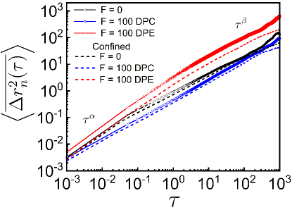
To test the robustness of our model of dipolar activity, we study the dynamics of a tagged monomer and the spatial correlation length of the polymer chain under spherical confinement of radius . The trends of and with the spherical confinement (see supplementary Fig. S9 and S10) are qualitatively similar with or without the spherical confinement. This suggests the spatial coherence in polymer primarily arises due to the correlated motion of the beads. However, the dynamics of the tagged monomer (see supplementary Fig. S9) and the COM (supplementary Sec. II and Fig. S2). are suppressed due to the confinement. Accordingly the spatial correlation length also decreases in the presence of confinement (see supplementary Fig. S10).
V Conclusion
Active forces inside a nucleus play an important role in both genome organization and dynamics. Experiments suggest that interphase chromatin is subjected to ATP-powered enzymes such as RNA polymerase [28]. Motivated by that, we implement the simplest two types of dipolar active forces, namely extensile and contractile on semiflexible, self-avoiding polymer chain. The main findings from our model are the following,
(1) The MSD of a tagged monomer for DPE system shows enhanced subdiffusion than the DPC one which is related to the shifting of peak values of distribution at large values of bond length in the DPE case. In our model, spatial coherence emerges with or without dipolar activity. However, the correlation length increases or decreases for the DPE or DPC system as compared to the case with no dipolar forces.
(2) Although we do not consider the hydrodynamic interactions, we show that how the local motion (related to tagged monomer’s dynamics) is associated with the large scale spatially coherent motion. Hence, the coupling between activity and elasticity (related to bending and stretching in our single polymer chain) generates the large scale spatially coherent motion. In other words, hydrodynamics is not essential to show large scale spatially coherent motion of chromatin. A simpler model like ours can capture coherent motion.
(3) In our model, we observe that the center of mass motion is not enhanced in the presence of dipolar active forces. This suggests that in this context, the effective temperature is not a good descriptor for dipolar activity. In that way, our model differs from typical active systems where one observes superdiffusion [5].
(4) Our work demonstrates that spherical confinement does not affect the qualitative trends of the spatial coherence. The dynamics of the tagged monomer is suppressed due to the confinement. Accordingly the spatial correlation length also decreases in the presence of confinement. The spatial coherence emerges from the correlated motion of the monomers.
(5) More importantly, we explicitly show that the extensile or contractile dipolar active system can not be mapped to a thermal system with renormalized elasticity. Thus, chromatin models based on purely equilibrium forces arising from polymer elasticity and interactions [41] can not account for the active motorized systems [42]. However, our model of renormalized elasticity should be verified with other values of .
A recent Optical experiment showed that chromatin movement is coherent over a length scale of and persists for seconds [28]. In order to make a comparison with experiment, we consider each monomer represents base pairs. Therefore, we assume the diameter of each monomer is approximately nm [27, 41]. Considering the nuclear viscosity cP [43] and , the Brownian time scale of single particle is coming out to be ms. From Fig. 2 F, one can see that for the extensile force of magnitude pN, the correlation length saturates at and persists for seconds.
The physics underlying the phenomena we report here relies on the motion of a long semiflexible polymer driven by the dipolar active forces. We do not take into account the full complexity of the chromatin packing [44, 45] or any salt-induced long-ranged electrostatic interactions [46]. From our work, it is however clear that the coupling between activity and elasticity (related to bending and stretching of our single polymer chain) is sufficient to qualitatively explain the experimentally observed large scale spatially coherent motion of chromatin. We hope that the simplicity of our model helps us understand the structural and dynamical behavior of the energy consuming processes in chromatin and allows one to add more complexity to the problem, such as nuclear lamina.
Acknowledgments
We thank Nir Gov and Guang Shi for many stimulating discussions. S.C. thanks DST Inspire for a fellowship. L.T. thanks UGC for a fellowship. R.C. acknowledges SERB for funding (Project No. MTR/2020/000230 under MATRICS scheme). We acknowledge the SpaceTime-2 supercomputing facility at IIT Bombay for the computing time.
Supplemental Material
VI Mean Square Displacement of the center of mass
The most straightforward tool for understanding the properties of motion from the trajectories is the mean square displacement (MSD). The time-averaged MSD of the center of mass (COM) is defined as from the time series of the position of the COM where is the total run time and is the lag time. The time-and-ensemble-averaged MSD of the COM is obtained as: where is the number of independent trajectories. The MSD of the center of mass (COM) diffuses freely at all times in the presence or absence of extensile and contractile activity (Fig. S1). In addition, all the active and passive are merging with each other (Fig. S1). However, in the long time limit, the dynamics of the center of mass of the polymer chain will be obstructed by the spherical confinement (Fig. S2).
VII Distribution functions of the radius of gyration
To further quantify the effects of the contractile and extensile active forces on the loci mobilities, we analyze the probability distribution, of the radius of gyration of the chain where . For smaller DPC and DPE activities, s are Gaussian and appear to be qualitatively similar to of passive system. But, s for high DPE and DPC forces show well-separated peaks (Fig. S4). For large DPC force, is Gaussian and sharply peaked at lower values of . The broader distribution of with peak at higher value of deviates from the Gaussian for large DPE force which accounts for the enhancement of stretching of the polymer chain. For the high DPC force, the deviation of the peak value of from the passive case is small as compared to the deviation for the DPE force. This small deviation for the DPC force is most probably due to the self-avoidance of the beads. To test the effect of self-avoidance as an energetic barrier, we compute the potential energy and the mean square fluctuation of the velocity , per particle of the polymer chain at each instant of time in the steady state. The velocity of a monomer over the integration time step is defined as . It is a quantity that can be measured experimentally by tracking the position of a chromosomal locus as a function of time [47] and has been extensively used to determine the nature of the stochastic process underlying the observed motion [33, 41]. PE per particle increases more for the DPC forces than for the DPE forces (Fig. S3A) as the effect of self-avoidance translates to an increasing potential energy barrier for the DPC forces. On the other hand, per particle increases more for the DPE forces than for the contractile forces (Fig. S3B) as the DPE forces show larger displacements than the DPC forces.
VIII Number fluctuations
To gain a deeper understanding of the underlying complex movement of the monomers, we investigate the number fluctuations. To compute the number fluctuations, we randomly select a number of small spherical probes of radius at different locations within the system. We then construct a histogram over different spherical probes and independent trajectories from which probabilities are computed. In equilibrium, the statistics of fluctuations in inside a small spherical probe volume follows Gaussian distribution. For small values of DPE and DPC forces, we find that the the probability distributions are indeed Gaussian (Fig. S5). For large DPC force, also exhibits the Gaussian distribution. For large DPC force, the peak of shifts towards a higher value of and the width of becomes narrower than the passive one (Fig. S5). Hence, large DPC force generates high density regions, leading to decrease in mobility. On contrary, for large DPE force, decays exponentially with indicating that DPE forces promote larger displacements of the system than the passive one.
| (DPE) | ||
| (DPC) | ||
| (DPE) | ||
| (DPC) |
 |
 |
| (A) | (B) |
 |
 |
| (A) | (B) |
References
- Gnesotto et al. [2018] F. S. Gnesotto, F. Mura, J. Gladrow and C. P. Broedersz, Rep. Prog. Phys., 2018, 81, 066601.
- Smrek and Kremer [2017] J. Smrek and K. Kremer, Phys. Rev. Lett., 2017, 118, 098002.
- Schaller et al. [2010] V. Schaller, C. Weber, C. Semmrich, E. Frey and A. R. Bausch, Nature, 2010, 467, 73–77.
- Winkler and Gompper [2020] R. G. Winkler and G. Gompper, J. Chem. Phys., 2020, 153, 040901.
- Osmanović and Rabin [2017] D. Osmanović and Y. Rabin, Soft Matter, 2017, 13, 963–968.
- Samanta and Chakrabarti [2016] N. Samanta and R. Chakrabarti, J. Phys. A, 2016, 49, 195601.
- Chaki and Chakrabarti [2019] S. Chaki and R. Chakrabarti, J. Chem. Phys., 2019, 150, 094902.
- Joshi et al. [2019] A. Joshi, E. Putzig, A. Baskaran and M. F. Hagan, Soft Matter, 2019, 15, 94–101.
- Chelakkot et al. [2014] R. Chelakkot, A. Gopinath, L. Mahadevan and M. F. Hagan, J. R. Soc. Interface., 2014, 11, 20130884.
- Shin et al. [2015] J. Shin, A. G. Cherstvy, W. K. Kim and R. Metzler, New J. Phys., 2015, 17, 113008.
- Goswami et al. [2022] K. Goswami, S. Chaki and R. Chakrabarti, J. Phys. A Math. and Theo., 2022.
- Le Goff et al. [2001] L. Le Goff, F. Amblard and E. M. Furst, Phys. Rev. Lett., 2001, 88, 018101.
- Brangwynne et al. [2008] C. P. Brangwynne, G. H. Koenderink, F. C. MacKintosh and D. A. Weitz, Phys. Rev. Lett., 2008, 100, 118104.
- Maji et al. [2020] A. Maji, J. A. Ahmed, S. Roy, B. Chakrabarti and M. K. Mitra, Biophys. J., 2020, 118, 3041–3050.
- Bajpai and Padinhateeri [2020] G. Bajpai and R. Padinhateeri, Biophys. J., 2020, 118, 207–218.
- Salari et al. [2022] H. Salari, M. Di Stefano and D. Jost, Genome Res., 2022, 32, 28–43.
- Natesan et al. [2022] R. Natesan, K. Gowrishankar, L. Kuttippurathu, P. S. Kumar and M. Rao, J. Phys. Chem. B, 2022, 126, 100–109.
- Andersson et al. [2015] R. Andersson, A. Sandelin and C. G. Danko, Trends Genet, 2015, 31, 426–433.
- Eaton and Zidovska [2020] J. A. Eaton and A. Zidovska, Biophys. J., 2020, 118, 2168–2180.
- Agrawal et al. [2017] A. Agrawal, N. Ganai, S. Sengupta and G. I. Menon, J. Stat. Mech., 2017, 014001.
- Maharana et al. [2012] S. Maharana, D. Sharma, X. Shi and G. Shivashankar, Biophys. J., 2012, 103, 851–859.
- Papantonis and Cook [2013] A. Papantonis and P. R. Cook, Chem. Rev., 2013, 113, 8683–8705.
- Shi et al. [2018] G. Shi, L. Liu, C. Hyeon and D. Thirumalai, Nat. Commun., 2018, 9, 1–13.
- Agrawal et al. [2020] A. Agrawal, N. Ganai, S. Sengupta and G. I. Menon, Biophys. J., 2020, 118, 2229–2244.
- Chubak et al. [2022] I. Chubak, S. M. Pachong, K. Kremer, C. N. Likos and J. Smrek, Macromolecules, 2022, 55, 956–964.
- Weber et al. [2012] S. C. Weber, A. J. Spakowitz and J. A. Theriot, Proc. Nat. Acad. Sci., 2012, 109, 7338–7343.
- Liu et al. [2018] L. Liu, G. Shi, D. Thirumalai and C. Hyeon, PLoS Comput. Biol., 2018, 14, e1006617.
- Zidovska et al. [2013] A. Zidovska, D. A. Weitz and T. J. Mitchison, Proc. Nat. Acad. Sci. U.S.A, 2013, 110, 15555–15560.
- Saintillan et al. [2018] D. Saintillan, M. J. Shelley and A. Zidovska, Proc. Nat. Acad. Sci. USA, 2018, 115, 11442–11447.
- Mahajan and Saintillan [2022] A. Mahajan and D. Saintillan, Phys. Rev. E, 2022, 105, 014608.
- Liu et al. [2021] K. Liu, A. E. Patteson, E. J. Banigan and J. Schwarz, Phys. Rev. Lett., 2021, 126, 158101.
- Ghosh and Gov [2014] A. Ghosh and N. Gov, Biophys. J., 2014, 107, 1065–1073.
- Put et al. [2019] S. Put, T. Sakaue and C. Vanderzande, Phys. Rev. E, 2019, 99, 032421.
- Bianco et al. [2018] V. Bianco, E. Locatelli and P. Malgaretti, Phys. Rev. Lett., 2018, 121, 217802.
- Eshghi et al. [2021] I. Eshghi, J. A. Eaton and A. Zidovska, Phys. Rev. Lett., 2021, 126, 228101.
- Weeks et al. [1971] J. D. Weeks, D. Chandler and H. C. Andersen, J. Chem. Phys., 1971, 54, 5237–5247.
- Prathyusha et al. [2018] K. Prathyusha, S. Henkes and R. Sknepnek, Phys. Rev. E, 2018, 97, 022606.
- Isele-Holder et al. [2015] R. E. Isele-Holder, J. Elgeti and G. Gompper, Soft Matter, 2015, 11, 7181–7190.
- Plimpton [1995] S. Plimpton, J. Comp. Phys., 1995, 117, 1–19.
- Shaban et al. [2018] H. A. Shaban, R. Barth and K. Bystricky, Nucleic Acids Res, 2018, 46, e77–e77.
- Di Pierro et al. [2018] M. Di Pierro, D. A. Potoyan, P. G. Wolynes and J. N. Onuchic, Proc. Nat. Acad. Sci. USA, 2018, 115, 7753–7758.
- Goychuk et al. [2014] I. Goychuk, V. O. Kharchenko and R. Metzler, PLoS One, 2014, 9, e91700.
- Hajjoul et al. [2013] H. Hajjoul, J. Mathon, H. Ranchon, I. Goiffon, J. Mozziconacci, B. Albert, P. Carrivain, J.-M. Victor, O. Gadal, K. Bystricky et al., Genome Res., 2013, 23, 1829–1838.
- Langowski and Heermann [2007] J. Langowski and D. W. Heermann, Semin. Cell Dev. Biol., 2007, pp. 659–667.
- Fritsch and Langowski [2011] C. C. Fritsch and J. Langowski, Chromosome Res., 2011, 19, 63–81.
- Cherstvy and Everaers [2006] A. Cherstvy and R. Everaers, J. Phys.: Condens. Matter, 2006, 18, 11429.
- Lampo et al. [2016] T. J. Lampo, A. S. Kennard and A. J. Spakowitz, Biophys. J., 2016, 110, 338–347.