A photospheric and chromospheric activity analysis of the quiescent retrograde-planet host Octantis A
Abstract
The single-lined spectroscopic binary Octantis provided evidence of the first conjectured circumstellar planet demanding an orbit retrograde to the stellar orbits. The planet-like behaviour is now based on 1437 radial velocities (RVs) acquired from 2001 to 2013. Oct’s semimajor axis is only 2.6 au with the candidate planet orbiting \nuoaabout midway between. These details seriously challenge our understanding of planet formation and our decisive modelling of orbit reconfiguration and stability scenarios. However, all non-planetary explanations are also inconsistent with numerous qualitative and quantitative tests including previous spectroscopic studies of bisectors and line-depth ratios, photometry from Hipparcos and the more recent space missions TESS and Gaia (whose increased parallax classifies \nuoacloser still to a subgiant, K1 IV). We conducted the first large survey of \nuoa’s chromosphere: 198 H-line and 1160 indices using spectra from a previous RV campaign (2009–2013). We also acquired 135 spectra (2018–2020) primarily used for additional line-depth ratios, which are extremely sensitive to the photosphere’s temperature. We found no significant RV-correlated variability. Our line-depth ratios indicate temperature variations of only K, as achieved previously. Our atypical analysis models the indices in terms of and includes covariance significantly in their errors. The indices have a quasi-periodic variability which we demonstrate is due to telluric lines. Our new evidence provides further multiple arguments realistically only in favor of the planet.
keywords:
methods: data analysis – stars: activity – binaries: spectroscopic – planetary systems – individual: Octantis – planet-star interactions1 Introduction
A decade or so after the first exoplanets were described (Wolszczan & Frail 1992; Mayor & Queloz 1995), radial velocity (RV) evidence for the first retrograde planet appeared from a very unexpected source, the compact single-lined spectroscopic binary Octantis (Ramm 2004). However, these RVs shared the same initial fate as those from which almost hosted the first acknowledged RV-discovered planet (Campbell, Walker & Young 1988; Walker et al. 1992). was eventually confirmed 15 yr later (Hatzes et al. 2003), and was then the shortest period binary with a planet ( yr) – about 20 longer than that for Oct. Both initial series of RVs led their discoverers to describe both planet and stellar rotation-related scenarios, the latter then being suspected as more likely causes. These two binaries have many other parallel details in their exoplanet histories and host star characteristics.111For example, and very significantly, both hosts were originally classified as giants, rare for early exoplanet claims – and both K0 III – which made a stellar origin for the RV signals more tenable. They also share a trivial near-polar declination detail: .
Host stars may provide evidence that a candidate exoplanet orbit is retrograde relative to the star’s rotation (which we label type-1), and if in a binary system, relative to the two stellar orbits (our type-2). The first acknowledged retrograde planet was HAT-P-7b, promptly identified using the McLaughlin-Rossiter effect (our type-1; Winn et al. 2009; Narita et al. 2009). This had been preceded in the same year by the first paper describing the conjectured planet , (Ramm et al. 2009; henceforth R09), which has proven to be much more challenging for establishing its reality beyond reasonable doubt. This is almost entirely due to the unprecedented geometry of the conjectured system, whose stars are separated by only 2–3 au with the circumstellar i.e. S-type planet about midway between (see e.g. Gong & Ji 2018; Bonavita & Desidera 2020; Quarles et al. 2020). Some details for Oct (HD 205478, HIP 107089) and its conjectured planet (based on the persistent RV cycle with a period d) are listed in Table 1 and Table 2. The parallax was recently updated from Gaia observations, and critically for the planet claim, increased by about 10 per cent (Gaia Collaboration 2018; Kervella et al. 2019 - whose work specifically includes nearby stars with stellar and substellar companions).222Thus \nuoais less luminous and should be classified closer still to a subgiant, K1 IV, as now is also (Hatzes et al. 2003; Fuhrmann 2004). § 3.5 will discuss this important revision.
The system’s geometry makes a prograde planet impossible (R09; Eberle & Cuntz 2010). An S2 (i.e. S-type, our type-2 retrograde) orbit has a significantly wider stability zone than its prograde equivalent (see e.g. Jefferys 1974; Wiegert & Holman 1997; Morais & Giuppone 2012).333With zero evidence for retrograde status we label the orbit type-0 i.e. prograde, and assumed if not stated. If the host provides evidence of both type-1 and 2 we would label it type-3 (1+2). The scheme is applicable to single star hosts i.e. type 0 or 1, and both S- (circumstellar) and P-type (circumbinary) planets (Dvorak 1986), i.e. type 0, 1, 2 or 3. This opportunity for ’s reality was first investigated by Eberle & Cuntz (2010), and subsequently by Quarles, Cuntz & Musielak (2012), Goździewski et al. (2013) and Ramm et al. (2016; henceforth R16), all of which found retrograde solutions with merit but without being conclusive. Meanwhile, however, multiple other tests demonstrate that all other explanations (e.g. measurement artefacts, stellar variability, Oct being a triple-star system) are substantially less credible than the planet (R09; Ramm 2015 - henceforth R15; and R16). If the planet is an illusion, \nuoaso far provides no evidence of its causative role other than the persistent precise cycle of so far 1437 RVs over 12.5 yr, and thus would have the alternative distinction of seriously confronting our understanding of stellar variability.444The RVs were obtained using two CCDs and different calibration techniques (-cell and thorium-argon spectra) and therefore also different reduction methods. No other star’s study using our instruments and methods provide any similar planet-like RVs. The primary star’s argument of periastron, , has not changed significantly in 95 yr so any claim that a hierarchical triple-star system is creating the planet-like RVs is also unfounded (see R09 and R16 for details).
| Parameter | Octantis A | Reference |
|---|---|---|
| Spectral typea | K1IIIb-IV | (1) |
| (mag) | (2) | |
| parallax (mas) | (3) | |
| (mag) | our calculation | |
| (mag) | (2) | |
| (Hipparcos mag) | (4) | |
| Mass ()a | , | (2), (5) |
| Radius ()a | , | (2), (5) |
| (K)a | , | (2), (5) |
| , | (1), (6) | |
| Luminosity ()a | (5) | |
| () | (2) | |
| (d)a | (6) | |
| Age (Gyr) | –3 | (5) |
| Observations (RVs)c | 1180 -cell, 257 CCF | (1), (5) |
| time span of RVs | (1), (5) |
| Parameter | Binary | planet, Ab |
|---|---|---|
| Companion Mass | ||
| Object class | , or WD | Jovian |
| 7.05 | ||
| (au) | ||
| d | ||
| 0.24 |
Goździewski et al. identify a small number of nearby mean motion resonances for coplanar S2 orbits in Oct including one at the period ratio 5:2, this having been qualitatively suspected in R09. The unprecedented strong interactions suggest resonance is likely to be a contributing factor for stability, as in other multi-body systems (e.g. Campanella 2011; Robertson et al. 2012; Horner et al. 2019; Stock et al. 2020). would never be confined to a typical narrow orbital path but would move endlessly throughout a rather wide zone as Eberle & Cuntz (2010) first illustrated, leading to significant challenges for competing models trying to characterize different orbital geometries (Panichi et al. 2017).
Many S-type planets have now been reported, though demands for any following an S2 orbit remains rare since the binary must be quite compact to lead to this conclusion. Scenarios that may create such orbits include star-hopping (Kratter & Perets 2012), perhaps facilitated by a scattering event, or significant system or orbital changes involving stellar winds, accretion/debris discs or evolution to a white dwarf (WD) companion (see e.g. Tutukov & Ferorova 2012). The WD scenario may have support for Oct from spectrophotometric observations nearly 50 yr ago (Arkharov, Hagen-Thorn & Ruban 2005). They reported unusually large variability ( mag) in the near ultraviolet (345 nm) in the 1970s. Of the 172 ‘normal’ and 176 ‘suspect variable’ stars they catalogued, only two others had larger , both in the latter group. This may be a clue to the nature of as it seems unlikely \nuoais the source.
The first close-planet candidate for a WD host was recently reported (WD1856+534; Vanderburg et al. 2020), discovered using NASA’s Transiting Exoplanet Survey Satellite (TESS; Ricker et al. 2015), another space mission that should help unravel the Oct mystery. WD1856 b’s orbit ( d), is presumed to be due to reconfiguration and migration processes (see e.g. Lin, Bodenheimer & Richardson 1996; Rasio & Ford 1996), which must have relevance for any orbitally retrograde planet. Together with mass loss/transfer processes inherent in WD evolution, these scenarios may further complicate attempts to understand but also provide some advantage since orbit reconfiguration (of the planet or the binary) would not require interaction from external or other internal masses, as anticipated with an unevolved secondary star.
Two other recent claims are also relevant here. Firstly, another S2-type planet, HD 59686 Ab, has been conjectured in this somewhat wider but rather eccentric binary (Ortiz et al. 2016; Trifonov et al. 2018; K2 III, au, ). Interestingly, HD 59686 B is also suspected of being a WD, leading Ortiz et al. to investigate one possibility that the planet formed from a second generation protoplanetary disc. It is tempting to speculate that Oct and HD 59686 may be two early examples of relatively compact binaries with WD secondaries that created S2-type planets. Secondly, the first planet in a binary more compact than Oct was recently reported (HD 42936, dwarf; au; Barnes et al. 2020). HD 42936-Ab is close to its host ( au) so both it and WD1856 b are assumed to have reconfigured orbits, but with no evidence demanding either be retrograde.
Understandable suspicion also persists that \nuoa’s RV signal may be due to undetected surface activity. Hatzes et al. (2018) repeated this concern after ’s anticipated single-planet claim disappeared after more RV data was acquired. Oscillatory convective modes (Saio et al. 2015) were instead promoted as the variable RVs more likely origin, just as Reichert et al. (2019) speculate for Aldebaran – instead of its conjectured planet (Hatzes et al. 2015). But unlike \nuoawhich is a relatively unevolved low-luminosity star (and so far has a persistent periodic RV signal), (, 50), and Aldebaran (, 40) typify the theoretical high-luminosity expectations of a star having these convective modes. Both are classified K5 III and are reminders of the potential complications such evolved stars, both real and mistaken (e.g. \nuoaand ) can present. Other radial and non-radial oscillations in stars similar to \nuoainstead have a complex power spectrum that complicate asteroseismology studies (see e.g. Dupret et al. 2009). This is not at all consistent with the planet-like RV signal \nuoahas provided to date. Hence, if \nuoais deceiving us, a more reasonable concern is that stars more similar to it are more likely to be creating well-crafted illusions, such as . This possibility would create significant complications for other exoplanet claims now and in the future, and perhaps not restricted to similar subgiants.
This background has motivated the photospheric and chromospheric studies reported here. Photospheric line variations are critical for RVs but also for the extremely temperature-sensitive method of line-depth ratios (LDRs; e.g. Hatzes, Cochran & Bakker 1998; Gray & Brown 2001; Kovtyukh et al. 2003; R15; R16). R15 and R16 demonstrate temperature constancy for \nuoato as little as K over 12 yr, with high consistency with the very low photometric variability recorded by Hipparcos (see Table 1). This latest LDR series is also relevant as, more or less concurrently, observations have also been obtained by NASA’s TESS mission which significantly support \nuoa’s photometric stability, as well as RVs from ESO’s HARPS spectrograph (Trifonov et al., in preparation).
Chromosphere activity of \nuoahas so far been limited to three eye estimates of the K line from each of two spectra (Warner 1969), a single spectrum of H & K (R09) and H-line indices from 17 spectra (R16). All three papers concluded \nuoahad minimal activity. Additionally, the Mg chromospheric emission-line study by Pérez Martínez, Schröder & Cuntz (2011) found \nuoa’s activity to be very near their sample’s empirically-derived basal flux of 177 cool giants. Here we report on two much larger series: 198 line indices from the H line and 1160 indices.
Our work allows \nuoato be characterized in further detail, providing new evidence for the planet since significant activity is again refuted. Even if the planet is eventually proven to be an illusion, which seems to be increasingly unlikely, our work adds to the fundamental knowledge of the star at the centre of this persistently challenging system.
2 Instrumentation and observations
The data analysed here were acquired in two series, one about a decade ago and the other over the past two years. Both series were obtained at the University of Canterbury Mount John Observatory using the 1-m McLellan telescope and HERCULES, a fibre-fed, thermally insulated, vacuum-housed spectrograph (Hearnshaw et al. 2002). The CCD was a detector cooled to C which recorded the \nuoaspectra with a resolving power . Further instrument details and our reduction methods for obtaining flat-fielded normalized spectra can be found in Ramm (2004), where the first tentative mention of the conjectured planet is made, and R16. Our reduction software (HRSP; see Skuljan 2004) automatically provides both vacuum and air wavelengths. To make other vacuum-to-air conversions we used the formulae of Morton (2000).
The older series comprises nearly 1200 spectra obtained from 2009.96–2013.96, i.e. four years, and allowed our chromosphere studies of the H line and . The spectra were almost all obtained using an iodine cell that reconfirmed the precise-RV planet-like signal (see R16). For our study, 1160 spectra were included in the final analysis, made possible by the higher at these longer wavelengths. The initial sample size for our analysis was limited to 700 spectra as the lines were not included in the first year or so of observations. More details of these data sets will follow in the relevant sections.
A smaller set of 135 spectra were acquired more recently, from 2018.34 until 2020.42 i.e. over about 25 months. As the cell was not used for these observations, we could not obtain further high-precision RVs but instead could use these spectra to obtain a new series primarily of line-depth ratios. The last spectrum obtained (2020.42; JD245 9002) has the highest of our entire series and was acquired to also extend that range of our spectra. The time span of all spectra considered here is from the first LDR spectrum, 2001.85, until this last observation i.e. yr.
3 Photosphere line-depth ratios
We first present the results from our line-depth-ratio analysis of the new spectra (2018–2020) and compare them to the previously published LDR results (2001–20013 ; R15 and R16) as well as again, the Hipparcos photometry (1990–1993). The LDRs demonstrate the continued thermal stability of \nuoa’s photosphere and so are a useful prelude to our chromosphere studies.
3.1 Old and new LDRs and corresponding temperatures
We used the same methods and pipelines employed in R15 and R16: specifically, for each of the 135 new \nuoaspectra we constructed 22 LDRs and their errors from ten spectral lines in the wavelength region 6232–6257 Å. The principal equations for these calculations are given in R15.
One significant advantage of LDRs is that they can be used to derive a star’s temperature – which brings additional benefits – using a series of calibration stars whose temperatures allow precise interpolation (see R15; their fig. 1). Further increases in accuracy and precision are achieved by modelling the influences of temperature and luminosity (i.e. evolution) using linear regression (Press et al. 1994; algorithm fitexy) leading to a modified LDR labelled MLDR (see e.g. Gray & Brown 2001; Catalano et al. 2002; R15). R15 reported an accuracy of K for recovering the 20 calibration stars’ temperatures but a precision as small as K for their 215 \nuoaLDRs, in excellent agreement with Gray & Brown (2001): their temperature precision from 92 giant stars was 3.9 K. Neglecting these influences can yield significantly poorer temperature statistics as Gray & Brown discuss in the context of other studies.
R15 summarizes the strong relationship between the regression line’s slope and the ratio’s error (see their sec. 4.1). The slope is an indicator of sensitivity of each ratio to the calibration stars’ temperatures. It therefore provides the error on each ratio’s temperature estimate i.e. . Fig. 1 (a) shows the error on each LDR eventually rises exponentially as the spectrum’s drops, as anticipated. We estimated the solely from the photon noise so that where is the continuum flux at the spectral line, and calculated each ratio’s from the average of the two lines. Our two examples show typical similarities and differences (the relationship illustrated here for the first time), and how can vary between ratios even though all the lines are within about 25 Å ( Å).
The 22 values next allow the mean and standard deviation, , for each spectrum to be derived, weighted by . Our average temperatures have no adjustment for any zero-point differences of the values for the 22 ratios. The mean values, , and their standard errors () are illustrated in Fig. 1 (b) and (c) respectively. The final standard deviations have an average K which is consistent with the temperature accuracy stated above.
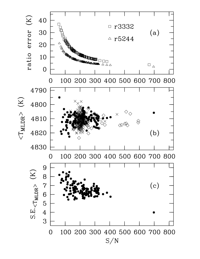
The total set of 398 values comprises 217 spectra from the first observing series (2001.85–2007.16, 84 nights; R15 and R16), 46 spectra acquired during the -RV campaign but without the cell (2011.22–2013.74, 20 nights; R16), and our data (26 nights). The distribution of all of these LDRs in terms of is provided in Fig. 1 (b). This shows that becomes less scattered as increases, particularly for , though this may just be an artefact of the smaller sample size. It can also be seen that all of the spectra with were obtained in our latest series.
3.2 Final temperature statistics and periodogram
The more recent 135 spectra give a weighted mean temperature K, with no significant difference from the values reported in R15 and R16. Our errors yield which indicates their average ( K) is somewhat more than what would be consistent with our tiny temperature variations. The three series combined have a weighted mean K. If the temperature-recovery accuracy given above ( K) is added in quadrature to this, the final temperature estimate for the 2018–2020 spectra is K, equalling the other two LDR temperatures in Table 1 – Ref. (1) and (6).
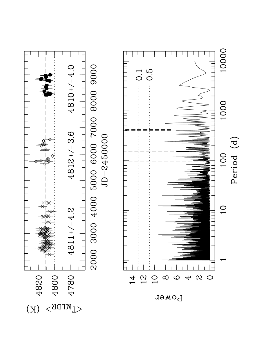
Fig. 2 illustrates the distributions of the mean values for the 130 epochs of the LDR spectra acquired over 18.6 yr. The means are weighted by the standard errors where we abbreviate with . Our results display an extraordinary degree of relative accuracy between the three series – the offset of the three mean temperatures is remarkably tiny at about 1 K (see values in Fig. 2). So whilst the absolute accuracy of LDRs may be less impressive, there is extraordinary relative accuracy even though their sensitivity may be imagined to make them vulnerable to variability from, for instance, measurement artefacts including subtle possibilities such as stray light within the spectrograph (which is unexpected given the design of HERCULES and that our line-depths create ratios). Clearly our methods provide practically identical MLDR distributions of outstanding precision over nearly 20 yr, despite two CCDs being used and many other instrumental and environmental parameters varying as well. Thus we can be quite confident our LDRs are highly unlikely to be significantly compromised by any of these non-stellar variables.
We searched our data for periodicity using the generalized Lomb-Scargle (GLS) periodogram as derived by Zechmeister & Kürster (2009). The GLS is ideal for time series with uneven temporal sampling and nonuniform measurement errors as reported here. Our periodograms are normalized assuming the noise is Gaussian (Zechmeister & Kürster; their eq. 22). In Fig. 2, we show the result for our epoch-averaged MLDR temperatures, along with approximate analytical -values estimated according to Sturrock & Scargle (2010). We find no evidence for statistically significant periodicity at any frequency.
3.3 Photometry from Hipparcos and TESS
We next make a brief digression to describe photometric satellite data which we will then compare to our LDR evidence. Since it has been estimated that is at least 6 mag fainter than \nuoa(R09, and see Table 2), the LDRs and photometry are assumed to only record \nuoa.
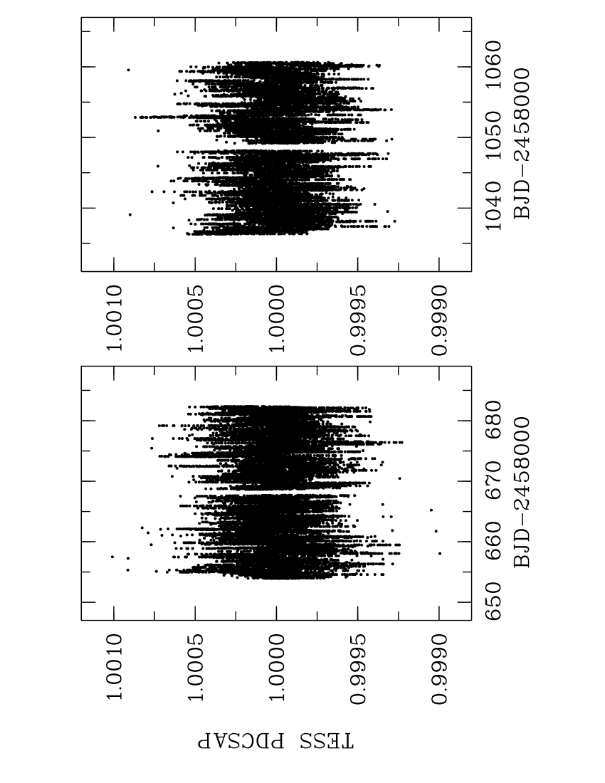
Two satellites observed Oct, acquiring data whose end dates are separated by 30.6 yr. The first, Hipparcos, achieved the longest baseline ( d, 1989.45–1993.17; ESA 1997) and identified \nuoaas one of its more stable targets (see Table 1). More recently, NASA’s TESS mission (Ricker et al. 2015) observed Oct twice in the 2-minute short-cadence mode. It was covered in Sectors 13 (2019 Jun 19 – Jul 18) and 27 (2020 Jul 5 – Jul 30), i.e. baselines of about 28 and 24 days. We retrieved the Pre-search Data Conditioning Simple Aperture Photometry (PDCSAP) using the Lightkurve software package (Lightkurve Collaboration, 2018). Approximately, this photometry has midtimes separated by 395 d and span 408 d. Therefore the two TESS records sample slightly different phases of the RV cycle (assuming d is still relevant), and together they include about 13 per cent of it. These high-precision records are also consistent with this bright spectroscopic binary being exceptionally quiet, at least during these short baselines and within TESS’s spectral response capabilities (600–1000 nm bandpass; Ricker et al. 2015): the RMS scatter of each PDCSAP dataset and both combined is just 0.02 per cent.
3.4 Magnitude differences from
The temperature calibration enables one more significant benefit: the values can be converted to a magnitude difference using the Stefan-Boltzmann law (). The Hipparcos and TESS photometry strongly support a claim that , and the LDR results just as strongly record . Therefore, though \nuoano doubt has some surface variability, as even less evolved stars do, we assume any radial changes are insignificant in our next calculation, a repeat of what was reported in R15 and R16. Eq. (1) provides the conversion to with that assumption (i.e. ):
| (1) |
where we abbreviate (i.e. K) with . Note that is extremely sensitive to the temperature: varying by only one degree changes by about one millimagnitude.
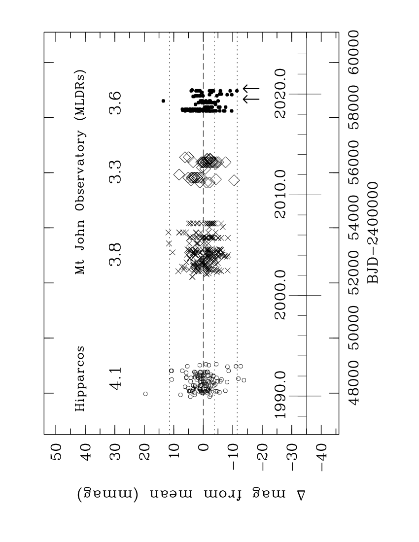
In Fig. 4 we compare these estimates to the magnitude differences for the longer baseline photometry of Hipparcos, whose values relate to their mean. A striking similarity is evident between the four distributions, all the more so as there are no zero-point offsets applied to any data. The latest MLDR series extends the time span of all values to about 30.5 yr. This graph also demonstrates that the more recent lower- data do not significantly compromise the precision of these values relative to the earlier data sets.
Finally we note the small difference between the standard deviations of and , where is greater than mmag. Of the various possible reasons one perhaps more interesting to speculate is that this small difference records the anticipated tiny contribution that would make to the Hipparcos photometry, but not our LDRs which are more directly sensitive to temperature changes. Our evidence for this is too slim for a credible claim but the idea might be successfully explored with more suitable data.
This completes our work with LDRs. It confirms past conclusions: \nuoacontinues to have a very thermally-stable photosphere, which is difficult to reconcile with surface variability as we presently understand its many variations. As discussed in considerable detail in the LDR work reported in R15, neither star spots nor pulsations are believable scenarios for creating the planet-like RVs in these circumstances. The same explanations there apply here.
3.5 Gaia and more clues negating a stellar origin for RVs
With the benefit of Gaia’s parallax (see Table 1) and our confirmation of the photosphere’s stable temperature, we can also review several parameters that have some relevance here. The Gaia parallax is about 10 per cent greater than the three values reported in R09, which includes that from Hipparcos (ESA 1997). Consequently \nuoa’s luminosity is less, which we now estimate is about 14 (and mag; Table 1). Based on the weighted mean of the five temperatures given above (i.e. K), \nuoa’s radius is also less i.e. (see R09, their eq. 3). The star is therefore now classified more closely as a subgiant, i.e. , and placed in a sparsely populated part of the H-R diagram (very near ), well-separated from the so-called instability strip and other known classes of pulsating stars. It remains to be seen if future revisions change this significantly.
Such a star is not known to have a rotation period anywhere near as long as that of the RV cycle i.e. d. In fact, the star’s (see Table 1), our revised estimate for the radius, and assuming the rotational and orbital axes are parallel, i.e. , predicts the star’s rotation period is d. R09 devotes their sec. 4.1.7 to the considerable improbability that rotation could be significant for the RV signal’s origin. This scenario was made even more difficult to believe when R16 doubled the time span of the persistent RV cycle to 12.5 yr, and is reduced even further by the new evidence presented here.
Finally, we assess if solar-like oscillations have any chance of influencing our observations of the now less-evolved \nuoa. One way is to apply the formulae from Kjeldsen & Bedding (1995), specifically equations 7, 8 and 10 to our new values for . Using the weighted mean for the stellar mass, such oscillations have a predicted velocity amplitude of about 2, a maximum-power period of only 1.5 hr and a luminosity amplitude ppm at 6000Å (the wavelength from Wein’s Displacement Law for the peak luminosity for our mean ). These values are in excellent agreement with the graphical ones in Dupret et al. (2009) who studied both radial and non-radial oscillations. One of their stellar models is slightly evolved and similar to \nuoa(their Case A, fig. 5, panel 3 at Hz). Its non-radial modes have smaller amplitudes than the radial ones, and together these produce a low-amplitude and very complex frequency spectrum, nothing like \nuoa’s planet-like RV signal. Such oscillations cannot have any significant impact on any of our data.
We now report our analysis of the chromosphere-activity indicators, the H line and , the study of which benefits from the long series of precise LDR results – any photospheric contribution to these indices is almost certainly insignificantly variable.
4 Chromosphere activity: and indices
Many spectral lines have been identified as being useful for monitoring chromosphere activity in late-type stars (see e.g. Lisogorsky, Jones & Feng 2019). One of the motivations for assessing such behaviour is the quest for increasingly precise RVs for exoplanet searches. Whilst many photosphere lines can be used as indicators for chromosphere activity, the classic ones with the strongest history are the resonance doublet lines of H and K at 3968.47 and 3933.66 Å close to the boundary of the ultraviolet and visible (see e.g. Wilson 1963; Linsky & Avrett 1970; Wilson 1978; Duncan et al. 1991; Baliunas et al. 1995). However, these two lines have the weakness, which will significantly influence our study, that they are recorded in spectral regions that have inherently low .
At the other end of the visible spectrum is ( Å). This has the distinct advantages of much higher than provided at H and K ( greater), and a better defined continuum without the complications of many neighbouring metal lines as H and K also have. However, as we will show, instead has the complication of telluric lines, and for a quiet star such as \nuoa, these lines dominate the line-index variability. The differences resulted in our having a final set of about 200 H-line indices but nearly six times as many indices.
4.1 Line index definitions including covariance
An index is a conventional method to assess variability of a suitable line’s core for evidence of stellar activity (for its earlier history see Griffin & Redman 1960). Our index, , includes the line’s core interval and two reference intervals and :
| (2) |
where each flux interval comprises bins having relative fluxes . Modern studies use either total fluxes or mean fluxes: the index derived from mean fluxes exceeds that from total fluxes by (if ). If total fluxes are used, the error on each flux . If mean fluxes are used , i.e. the standard error on the mean, which ensures the index’s relative error will be identical to that from total fluxes. We will always use mean fluxes.
The index error was calculated using error propagation:
| (3) |
where we introduce the error symbols here and below for future reference. Whilst this is the typical calculation for such an index, Eq. (3) may be incomplete since the flux errors are calculated from the fluxes which, if suitably chosen, should be highly correlated. This suggests covariance deserves consideration.
The expression for the total covariance must be added to Eq. (3):
| (4) |
where is a correlation coefficient, represents the sum of the reference fluxes, and is calculated by also including its covariance term, i.e.,
| (5) |
The sign of and will determine if and/or increase or decrease the total error, or if . If only one reference interval is used and covariance taken into consideration, the contribution of to the total error is absent.
4.2 H line spectra and data set
When seventeen H-line indices were reported in R16, the spectra we analyse here were available. However, most of the 700 archived spectra, have quite low (), and previously had been considered probably useless for any definitive study based on expectations and a preliminary sample’s analysis.
As a definitive understanding of the Oct system is yet to be attained, we took a second look at this large pool of spectra to review the earlier decision. We decided that it was a poor strategy to co-add spectra since the few available for most nights result in very little advantage and co-adding many across multiple epochs would provide fewer final indices, most obtained with greater complication and risk for errors as for instance Zechmeister et al. (2018) warns. Instead, a rather more novel approach was undertaken when a distinctive distribution that could be modelled revealed itself from a larger sample of indices.
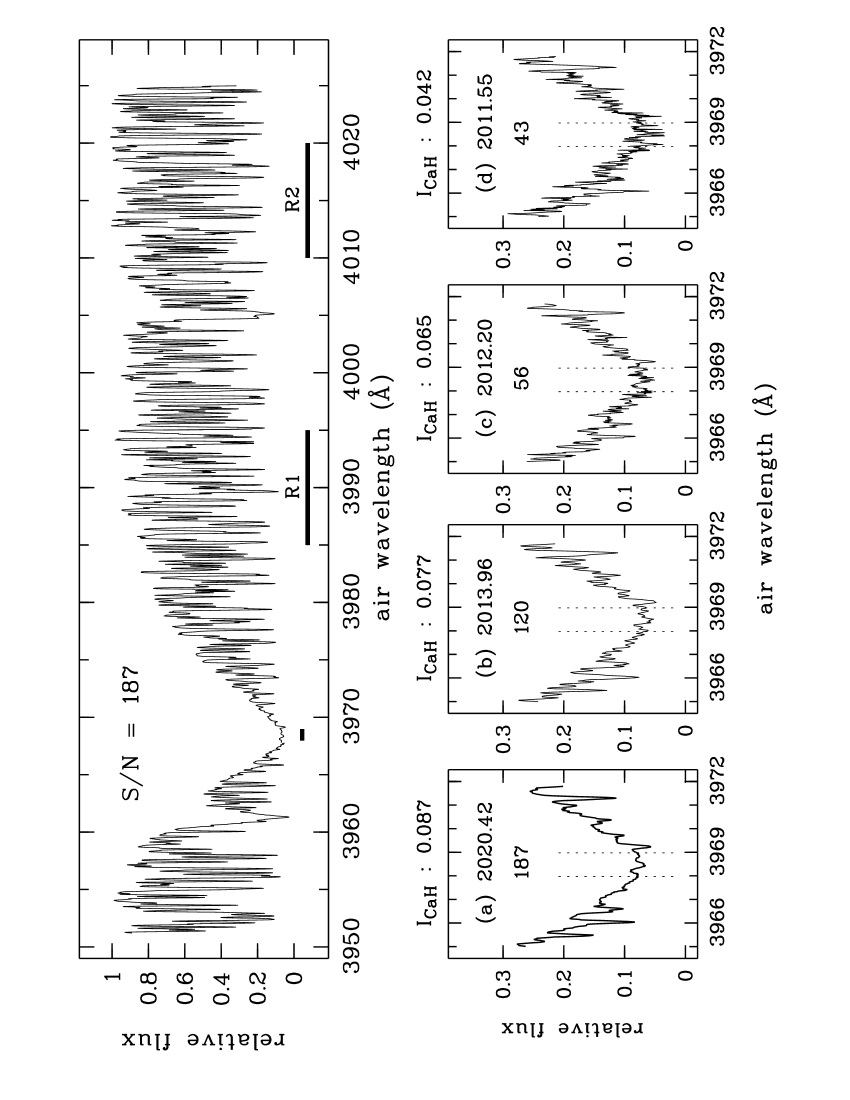
The HERCULES archive provided an initial sample of 482 spectra. Many of the original 700 spectra could not be properly processed due to more prevalent cosmic rays and other complications. We restricted our analysis to the record of the H line in as its is about 40 per cent greater than its duplicate in and both records of K. The 218 discarded spectra have at the H line record we used. Four H-line spectra of varying are illustrated in Fig. 5 showing \nuoa’s minimal chromospheric activity and the extent of slight infilling which varies primarily due to spectral noise.
4.2.1 Preliminary indices and errors
The origin of the dominant chromospheric flux is in the vicinity of the temperature minimum (Linsky & Avrett 1970) which is presumably highly correlated with the LDR temperatures just described. The H line has variable amounts of infilling and activity depending on, for instance, the star’s luminosity (Wilson & Bappu 1957). Typically the H-line core of main-sequence stars is sampled with an interval of about 1–1.1 Å (e.g. Wilson 1978; Duncan et al. 1991; Cincunegui et al. 2007; Boisse et al. 2009). The residual photospheric contribution which complicates accurate measurements of only the chromospheric component, for instance for surveys with different spectral types and luminosity classes (see e.g. Oranje 1983; Rutten 1984) can be neglected here since we are studying only \nuoa, which in any case has a very thermally-stable photosphere from evidence summarized in Fig. 2.
Our H-line cores have a width of about 1.0 Å; see Fig. 5. This detail provides further indirect evidence for \nuoa’s revised less-evolved luminosity class (see § 3.5). Rather than commit to a single interval width we used a series in 0.1 Å steps from 0.9 Å to 1.5 Å. We selected two reference intervals, R1 and R2, each 10 Å wide, centered at Å in order and at Å in order (see top panel Fig. 5). The second redder reference interval was chosen so that it would have a slightly higher motivated by our mostly low-quality spectra.
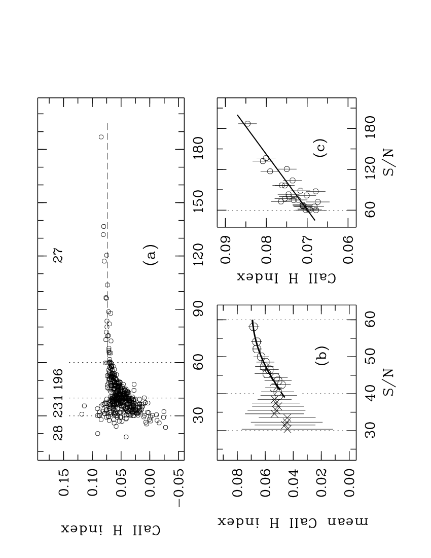
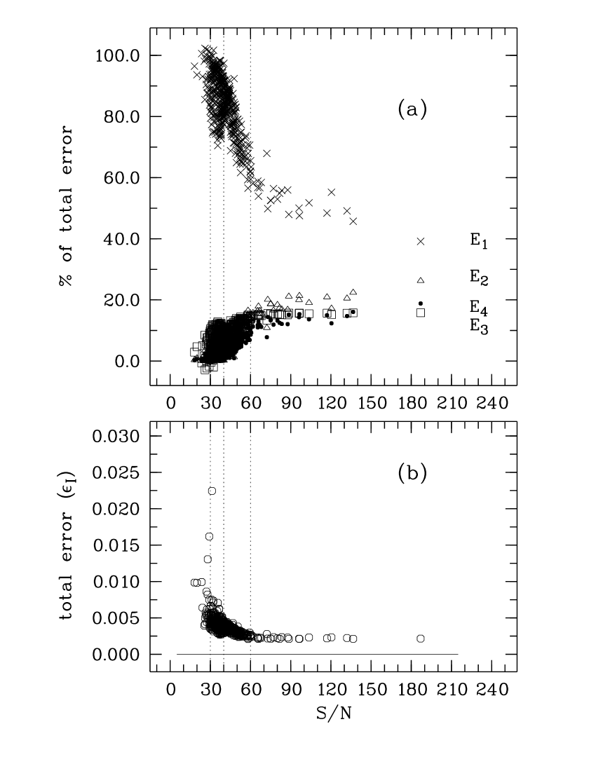
Our preliminary 482 indices are shown in Fig. 6 (a), given in relation to their . These distributions fall into four ranges delineated by the vertical dotted lines in each panel at , 40 and 60. In Fig. 6 (a) the anticipated near constancy of the indices for a quiet star such as \nuoais evident for . The distributions of and their sum are illustrated in Fig. 7. Our errors yield and , so that both and are positive, and is about as significant as . is always the dominant term, but its contribution decreases as increases. The error terms tend to plateau just above the threshold , particularly for and . Below this threshold, the total error increases exponentially (Fig. 7b), and above it, the minimum errors begin and average . This error, incorporating the covariance terms, is equivalent to about 3.4 per cent of the index and about greater than the error without covariance included, a significant difference.
4.2.2 Modelling the trends in Fig. 6 (b) and (c)
The apparently near-constant 27 indices with in Fig. 6 (a) in fact delineate a fairly well-defined sloping line as shown below in Fig. 6 (c), even without the high- anchor. This we modelled with a linear fit weighting each index by to give our modified indices:
| (6) |
where represents and is the weighted mean of these 27 indices and defines our zero-point for . Note that if our spectra had limited to [60, 90] the implied slope of the distribution would disappear. The modelled indices have larger errors determined by the rescaled original index error created by the fitting process, the RMS of the linear fit (which varies with the core width of the H line), and the standard deviation of the original mean , each added in quadrature.
It is impossible to guess what the average behaviour of the 427 indices is in the interval [30, 60] in Fig. 6 (a), so we created a series of narrow bins, typically with . Starting at we extended the range in one unit steps until we had at least ten indices in each bin. This provided 23 bins. For each bin we calculated the average and standard deviation of the and the indices, each index weighted by its error as above. These statistics, in relation to each bin’s mean are plotted in Fig. 6 (b).
For the indices are adequately fit by a parabola. This fit though requires further care as it is not obvious what is its lower limit, which we label as . Its choice is another balancing act between precision and sample size for our final time series since the binned indices have increasingly higher standard deviations as decreases. We discarded 221 spectra in ten bins with as they have the largest standard deviations and are least consistent with our intended parabolic fit (marked with crosses ‘’ in Fig. 6 (b). For the 13 remaining bins, which include 261 original indices, we calculated the model-fitted final indices and their errors for core widths of Å. These four widths encompass those considered most suitable for our spectra (i.e. 1.0 and 1.1 Å; see Fig. 5).
4.2.3 Final indices and errors and their
Of the original 700 archived spectra, per cent are discarded from our complete analysis which somewhat vindicates the decision several years ago. Our errors and indices are now final. The errors each comprise two conventional terms and , two covariance terms and and three terms from each model depending on the spectrum’s , making a total of seven terms. Each error is approximately doubled by the model-fitting calculations.
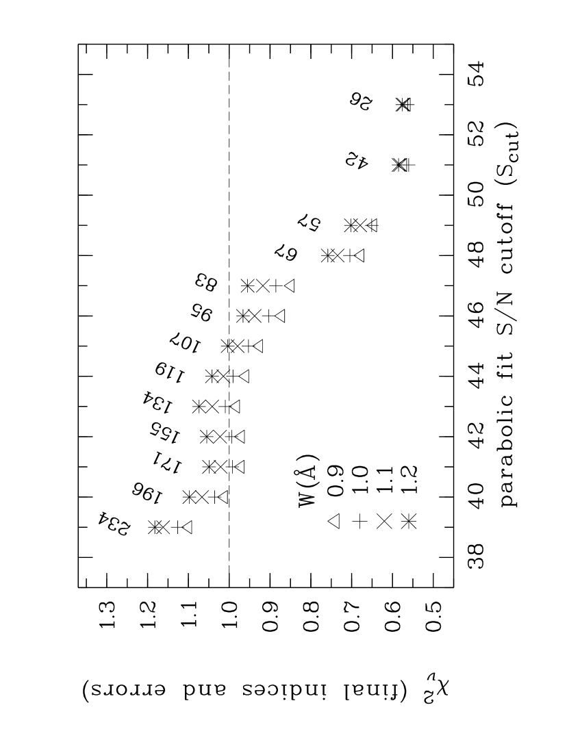
We calculated for our final indices and errors for our grid of four H-line core widths and thirteen values. Fig. 8 shows that our atypical analysis of mostly low- spectra and the inclusion of covariance ultimately provides strong evidence for the consistency of our indices, errors and models. For example, for the H-line core width Å, for the four consecutive parabolic fit thresholds . Without covariance . Our final relative errors average about seven per cent for the 198 indices defined by . In Fig. 9 we illustrate our final indices and errors for the time series defined by and Å which corresponds to . This example is approximately normally distributed as the lower two panels illustrate. We also derived for the 27 indices from the spectra with .
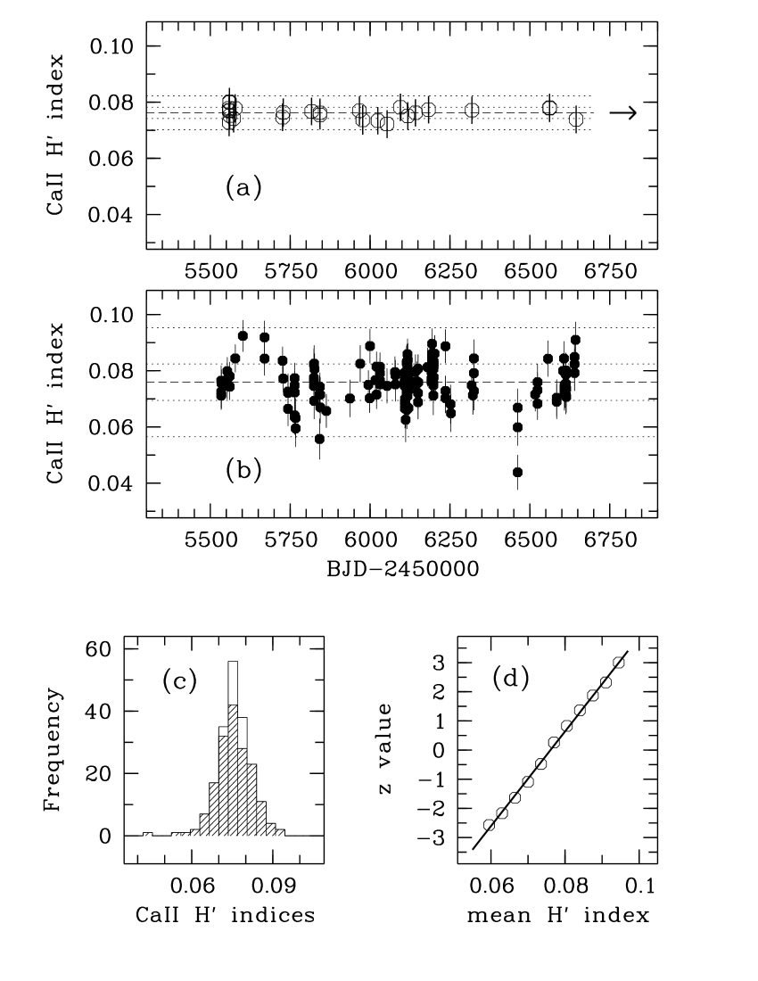
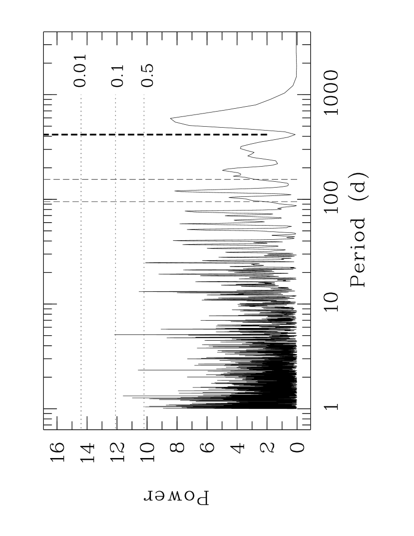
As we found with our LDR work, within our errors, there is nothing here that suggests anything but quite randomly distributed data, regardless of the temptation to perhaps imagine some significantly periodic behaviour in Fig. 9 (b) where removal of only a very few data points would make such a suspicion far less likely. Our GLS periodogram search as described in § 3.1 confirms this (see Fig. 10). It was created using the indices plotted in Fig. 9. There is no significant peak corresponding to \nuoa’s predicted rotation period ( d) or the planet-like RV period ( d) where a deep trough is in fact evident. Unfortunately, our lack of any detection of a credible rotation period (both here and with our LDR data) means we are still limited to estimates of as in Table 1 and § 3.5 (where, in any case, we noted rotation remains a highly unlikely explanation for the RV cycle).
4.3 spectra and data set
’s unique planet claim demands certainty about any conclusions relating to any index variability similar to the RV signal. Our indices have this characteristic, having a quasi-periodicity in the vicinity of the conjectured planet’s period. We intend to provide robust proof that this is caused solely by telluric lines.
is a prominent photospheric absorption line in late-type stellar spectra. Its core can also include chromospheric activity. It was this profile variability that led to being studied for Cephei in 1979 using one of the first digital detectors, an experimental Fairchild CCD (Young, Furenlid & Snowden 1981).
We employed a long time series of indices as densely sampled as possible, corresponding to the -cell RVs reported in R16. Such a sample is critical for demonstrating the cause of the dominant variability in our indices. The 1160 spectra archived over four years comprise 229 epochs. Thirty spectra (from 18 epochs) were acquired without which are useful to compare our indices with and without involvement. For the majority with lines, our cell benefited from a temperature controller designed to minimise variability ( C), so that the density and extent of the forest was assumed to be quite constant.555We will discuss the absence of any significant impact of the forest on our indices in the final paragraph of § 4.3.2. is recorded in two HERCULES spectral orders, and 87. The in order 87 is about twice that in 86 so we used only , their range at being and their mean 220.
Our first evidence of the role of telluric lines is presented before indices are calculated. The high region where resides is also uncomplicated by large numbers of other photospheric lines such as the metal lines near H and K. It is therefore very suitable for making a preliminary visual comparison of all of our spectra with respect to a reference. This has the advantage that the entire region can be assessed for significant flux variations which may be concealed by the solitary line index. We ensured all our spectra have an essentially level continuum with a maximum relative flux , and that each core centre is measured accurately to within a pixel by also comparing the fitted centre of the sharp line ( Å) redward of with each core fit. We calculated the relative flux differences between each spectrum and our reference (see Fig. 11).
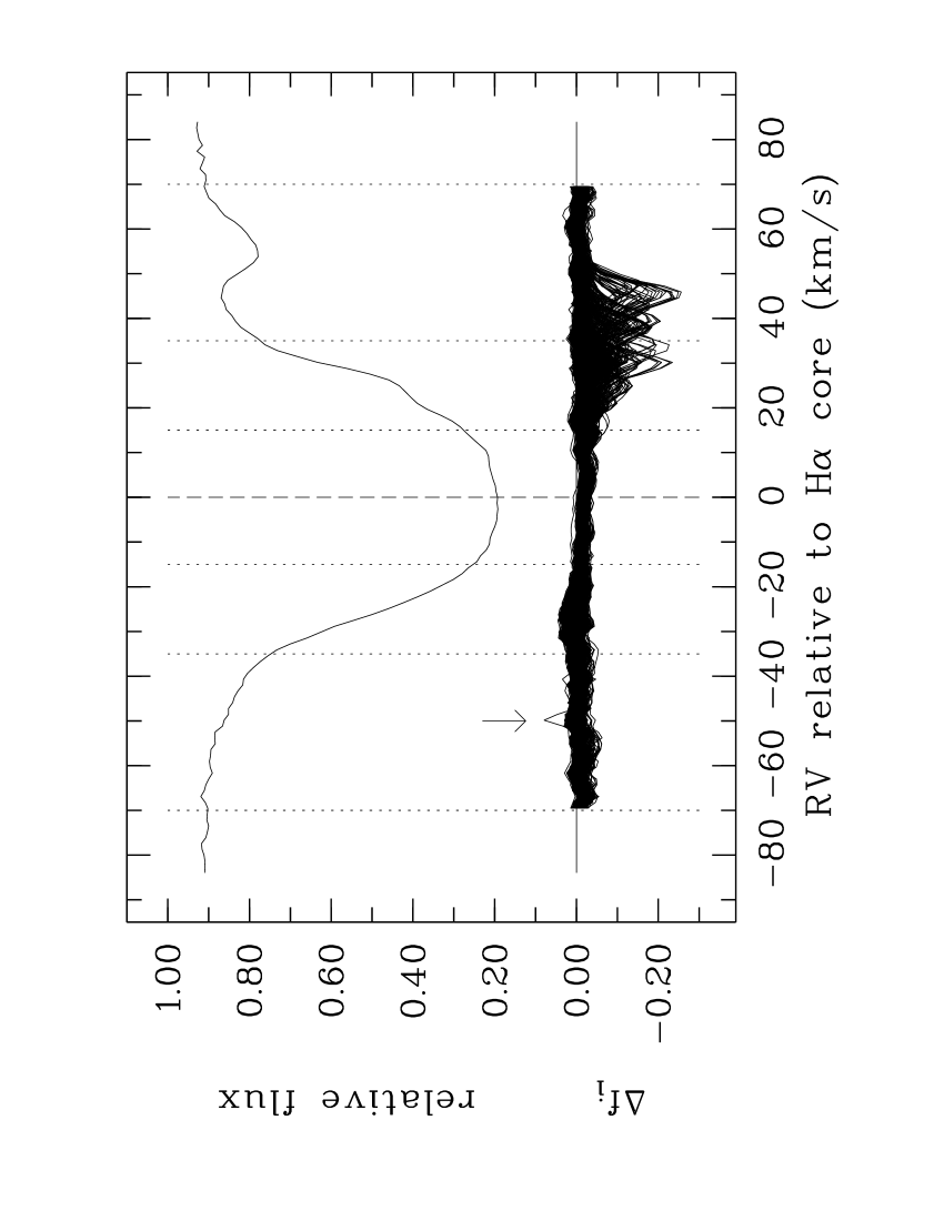
This plot alone is strong evidence that has very little core activity since the variations for the core interval are actually the least of the wide range shown. Instead we see time-dependent line movement contaminating both shoulders of , but particularly the redward one, which subsequent evidence will prove are telluric lines. We were fortunate that the strongest telluric lines did not engulf our line cores as may occur in other circumstances.
4.3.1 Non-stellar lines and \nuoa’s absolute RV
All of our spectra include telluric lines and most also the forest. An example of these non-stellar lines in a HERCULES spectrum of the fast-rotating Be star Achernar ( Eri, B6V, ) is provided in Fig. 12. About a dozen prominent telluric lines are recorded but the region includes many more fainter ones.666For instance, within the 95 Å shown in Fig. 12, the online database HITRANonline (https://hitran.org) lists 576 water vapour lines, the principal species contributing to the telluric spectrum. For details of its latest release see Gordon et al. (2017).
’s absolute RV is intimately connected to the relative behaviour of its lines and any non-stellar lines. We measured the absolute radial velocity () of \nuoausing the shift from the rest wavelength of the line at Å. This line is recognized for its relative stability (e.g. Kürster et al. 2003; Robertson et al. 2013), and for our purposes, the resulting low-precision RVs are adequate. Our estimates and the best-fitting curve are provided in Fig. 13. Vertical lines identify the RV minima which have different time spans between them making them ideal for connecting the variations to our index variations that we will next describe. Note that all of the intervals differ from the orbital period of the conjectured planet and the predicted rotation period of \nuoa, and critically, the differences are due to \nuoa’s orbital RVs that a single star would not provide.
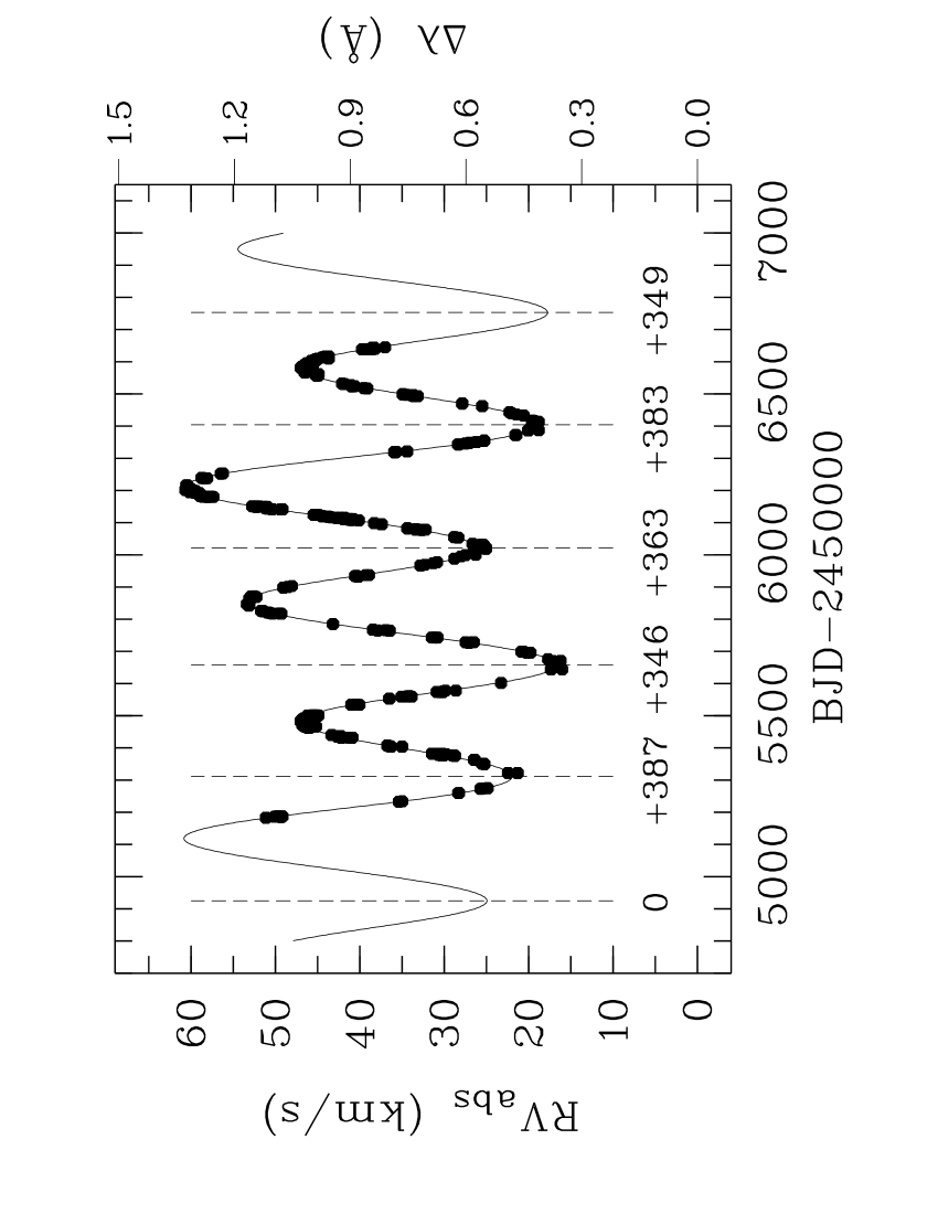
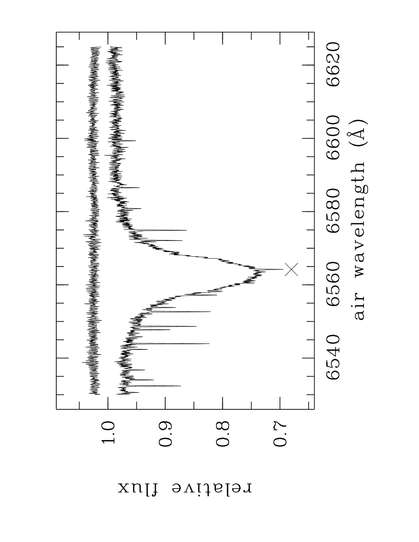
Fig. 14 includes the spectrum with the highest , a cartoon representation of the strongest telluric lines recorded in Fig. 12, and identifies the line. The reference intervals R1 and R2 are defined in the next section.
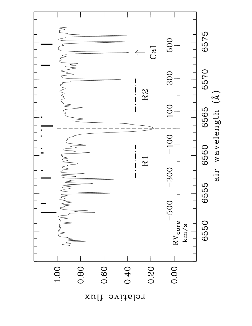
4.3.2 indices
The literature describes many choices for the flux intervals for indices. For a survey of their variety see e.g. Kürster et al. (2003); Cincunegui et al. (2007); Gomes da Silva et al. (2011); Ortiz et al. (2016); Zechmeister et al. (2018). We used three core widths, with the centre defining the RV zero-point for all flux intervals. The narrowest, , is suggested by the evidence in Fig. 11, and is similar to that used by Kürster et al. (2003). We also included the wider interval (similar to Zechmeister et al. 2018) and one twice that, , chosen to be just beyond the maximum absolute RV of \nuoa( ). We used the two reference intervals R1 and R2 defined by Zechmeister et al. (2018), namely and and calculated the index errors including covariance as described earlier.777We also calculated all of our indices using the reference intervals defined by Kürster et al. and Cincunegui et al., which are distinctly different from Zechmeister et al. These index distributions were indistinguishable for the narrowest core width and barely so for the mid-width core. The indices we derived with the Zechmeister et al. reference intervals were significantly more precise for the widest core interval, which is why they are reported.
Unlike our indices, there is no correlation between and our indices (). However, none of the index distributions (see Fig. 15) appear to be strictly random – they all have evidence of cyclic behaviour with the dominant period of about one year, although this doesn’t become better defined until the index uses the two wider regions, the main reason for their inclusion. Only the widest core width provides a significant maximum peak power in a periodogram and this is at 365.5 d (coincidently the mean of the approximated timespans in Fig. 13 is 365.6 d). This quasi-periodicity close to one year strongly implies the primary cause has a non-stellar origin, i.e. telluric lines.
For the first time we demonstrate the usefulness of the five minima lines as evidence that telluric lines are the dominant cause of our index variations: the set of lines has been offset in time by d for the core width but unadjusted for the widest one, and these included in Fig. 15 for the top two panels. Not only is adequate alignment found, simply made by eye, but the two offsets are unequal. The relative contributions of stellar and telluric lines vary if the flux intervals differ and this explains why the time shift to make this alignment is unequal for the two wider core widths that we can more easily assess – in fact, for this reason, it is also more likely the shifts will differ. The more precise index variations of the widest core interval is perhaps explained by the more prominent roles of both the very stable photosphere and the additional telluric lines found here (which are also present in the reference intervals).
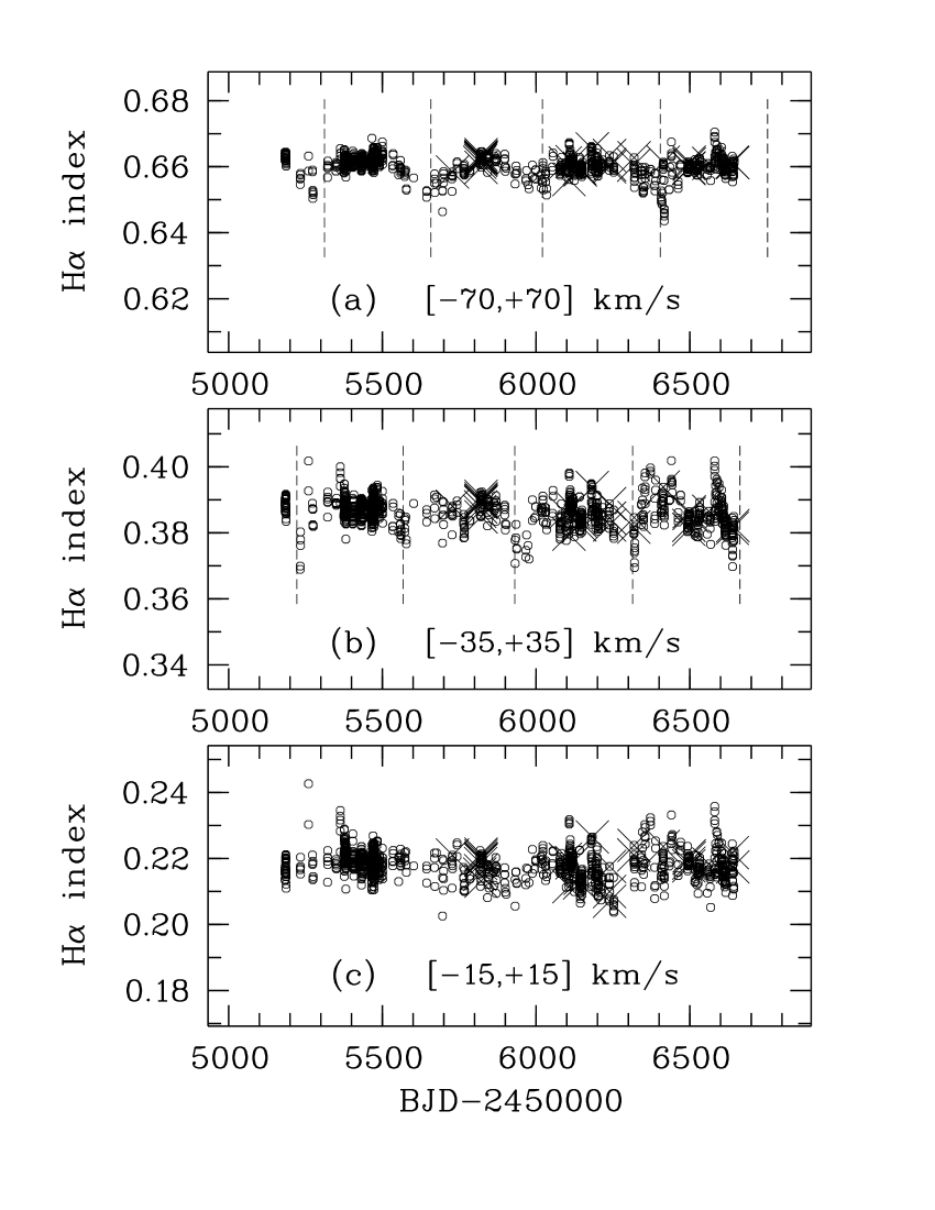
Thirty spectra were acquired without the cell, the benefit of which is also clear from Fig. 15: the no- indices have a distribution that is consistent with those with . To confirm this similarity, we also derived indices from our 135 new spectra (used for our LDR study) whose spectra also have no lines. Their distribution is far less dense and uniform than our much larger series (which is the principal reason the former were not otherwise included for ) but are statistically indistinguishable from that derived from spectra with . This demonstrates that the previous concern for using spectra including the forest for an study was unfounded, and duplicate the claim made in Kürster et al. (2003) that involvement made no significant impact on their and indices for Barnard’s star. That the complete absence or inclusion of lines makes no significant difference to these indices also makes it clear that any temperature variations of the cell leading to variability of the forest’s extent is highly unlikely to make any difference either.
4.3.3 Other evidence
Several more pieces of evidence ensure our variations are dominated by telluric lines. Firstly, Bergmann (2015) used HERCULES to also measure indices for Cet, Pav and Cen A and B in the same time span and frequently on the same nights as our \nuoaspectra. These indices use a wider core interval and different reference intervals but still those distributions and ours are very similar. Bergmann’s four stars and \nuoaall have similar ranges ( ) so all had moving relative to telluric lines in quite similar ways. Secondly, Bergmann’s strategies to manage stray-light contamination between Cen A & B were strictly defined by his evidence his distributions were also substantially due to telluric line involvement, and more specifically, water vapour. Thirdly, Bergmann’s reduction pipeline differed from ours so the chances of the two duplicating a reduction artefact is also highly unlikely.
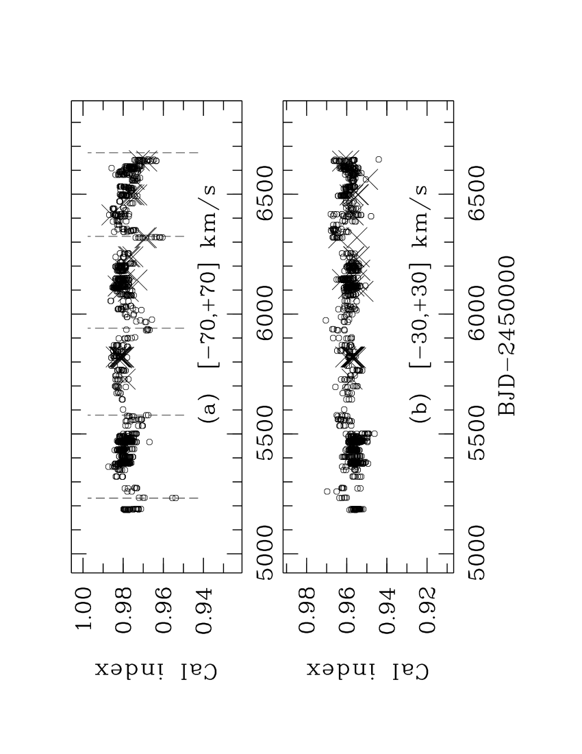
The final evidence comes from indices of the recognized ‘stable’ line used for our absolute RV estimates. We also calculated these using a series of core widths: the interval that is very similar to that used by Kürster et al. and Robertson et al. (2013) for their indices, and a series in 10 steps from 10–70 . We found provided the least variation (half that provided by ). Again, the core interval recorded most distinctly the influence of telluric lines (see Fig. 16). Note that this wider interval is more than the separation of the two strong telluric lines bounding in Fig. 14, and so both influence some indices. Our minima lines are again successfully aligned to the dominant cycles for the wider core interval. These results show that 1. the index distribution of the stable line closely mimics our indices and has the least variation of all our indices (the mean for is 0.3 per cent), and 2. if confirmation of stability is desired, or any other line is best studied when less likely to be contaminated by tellurics.
4.3.4 index errors and final comments
We calculated our index errors using the same methods described in § 4.1. Given the significant impact of the covariance terms and to our index errors, it was somewhat surprising that they make little difference to our errors, since the mean fluxes of the reference intervals are again highly correlated, just as they were for our indices (: ). However, perhaps related to the influence of telluric lines, the associated errors () are not at all highly correlated, regardless of the core or reference intervals used, since we also checked this result with the Kürster et al. reference intervals. If this result is common in other index studies it shows that the absence of the covariance terms also made no significant difference to their errors.
The core width that is most suitable for our original purpose – assessing ’s activity – is the narrowest one, . That index distribution is in the bottom panel of Fig. 15. is again by far the dominant error term. The relative contributions of the four error terms to their total are (0.962, 0.046, 0.005, ). The relative total errors have a mean per cent which yield . Both and are practically zero for two different reasons: as , and primarily because the error portion is (and , so that actually reduces the total error, but only insignificantly).
That we can precisely correlate the tiny effects of telluric lines in terms of suggests our methods are reliable and any activity is likely to be significantly less. Also, as a final minor detail, having established the origin of the dominant variations, we can now speculate that contributions to the almost nightly variations may be differences with the observations’ airmasses and the humidity that the telluric lines’ primary component, i.e. water vapour, also records.
5 Conclusion
We report five new independent series of precise data that all indicate \nuoais a very quiet star: two photometric series from TESS (2019, 2020), which more or less coincide with our LDR study of its photosphere (2018–2020), and our two large surveys of its chromosphere whose origin is the -cell RV time series (2009–2013). The TESS photometry bounds the 1437 RVs (2001–2013) with Hipparcos observations three decades before (1989–1993). A sixth line of new evidence is the Gaia parallax that indicates \nuoais less luminous, and so more probably approximately K1 IV. This also strongly favours the quiet-star classification, as does our review of solar-like oscillation scenarios. These results are consistent with all previous surveys, for instance, more recently, two bisector studies (R09 and R16), and two other LDR studies (R15 and R16).
There is no significant variability of any of these many photometric or spectroscopic time series, and certainly none correlated with the planet-like RVs. Other facts are against Oct being a heirarchical triple-star system or the cause being related to \nuoa’s rotation. Thus this overwhelming evidence demonstrates all non-planetary solutions continue to be implausible, which instead we interpret is only compatible with a retrograde planet whose properties are approximated in Table 2.
With thousands of planets now described, remains unprecedented in terms of the system’s geometry. It still provides many opportunities for exploring unexpected dynamical models of planet formation and orbit stability, as well as exceptional observational opportunities for such a bright, short-period system’s orbital behaviour. Recently found evidence that the secondary star may be a white dwarf was reported in the Introduction which would have a significant bearing on such studies. As more evidence accumulates only in favour of the planet, the flip-side of irrefutable evidence that the planet is instead an illusion is how unexpected any non-planetary alternative would then be.
We began by confirming how thermally-stable \nuoa’s photosphere continues to be. This allowed us to confidently claim the photosphere, which has produced the enigmatic RVs for over a decade, is highly unlikely to contribute any variability to our chromosphere indices, nor be the source of the planet-like signal. Knowing the thermal stability of the photosphere is a useful advantage for any chromosphere study, a detail not commonly reported.
It is no doubt partly due to \nuoa’s quiescence that has allowed our study of its spectra with such low and successfully pursue our atypical methods. It is also this stability that has helped us critically examine the telluric line contribution to our spectra and quite clearly reveal its quasi-periodic behaviour and origin. All our results strongly imply they record mostly random processes and not something systematically cyclic.
Because similar studies use data that may be at least moderately correlated it seems that covariance deserves closer scrutiny in such cases. Even though the covariance terms have opposite signs, the correlation coefficients may still cause the covariance terms to increase the errors significantly – as our results demonstrate. Our methods for analysing low- spectra may allow other so-far neglected archival material to be recovered usefully as we quite surprisingly achieved here. Finally, we introduced a simply described classification system for retrograde orbits that appears effective for our purposes, and may be of sufficient merit for use by others.
Acknowledgements
We appreciate the anonymous referee’s several suggestions that led to helpful improvements. DJR thanks M. F. Reid, then Physics & Astronomy HoD, for renewing his Research Fellow status (2018–2020) allowing continuing access to academic and IT resources including the assistance of O. K. L. Petterson. DJR is also grateful to the UC Mt. John Observatory director K. R. Pollard and the present HoS R. Marquez for the generous allocation of observing time and research support for this project that provided us the opportunity to obtain more data for Oct. We thank the observing technician F. Gunn for obtaining the spectra 2018–2020 and K. R. Pollard and R. Marquez of the School of Physical and Chemical Sciences, University of Canterbury for sourcing observing and technical support for this project at the UC Mt John Observatory, including funding from The Brian Mason Trust, UC Foundation, The School of Physical and Chemical Sciences and The Otago Museum. DJR thanks M. Kürster (MPIA) and K. J. Moore (Christchurch) for helpful contributions. This research made use of Lightkurve, a Python package for Kepler and TESS data analysis (Lightkurve Collaboration, 2018).
Data Availability
The data underlying this article will be shared on reasonable request to the corresponding author.
References
- Arkharov et al. (2005) Arkharov A. A., Hagen-Thorn E. I., Ruban E. V., 2005, Astron. Rep., 49, 526
- Barnes et al. (2020) Barnes J. R. et al., 2020, Nature Astronomy, 4, 41
- Baliunas et al. (1995) Baliunas S. L. et al., 1995, ApJ, 438, 269
- Bergmann (2015) Bergmann C. M., 2015, PhD thesis, Univ. Canterbury
- Bonavita & Desidera (2020) Bonavita M., Desidera S., 2020, Galaxies, 8, 16
- Boisse et al. (2009) Boisse I. et al., 2009, A&A, 495, 959
- Campbell et al. (1988) Campbell B., Walker G. A. H., Yang S., 1988, ApJ, 331, 902
- Campanella (2011) Campanella G., 2011, MNRAS, 418, 1028
- Catalano et al. (2002) Catalano S., Biazzo K., Frasca A., Marilli E., 2002, A&A, 394, 1009
- Cincunegui et al. (2007) Cincunegui C., Díaz R. F., Mauas P. J. D., 2007, A&A, 469, 309
- Duncan et al. (1991) Duncan D. K. et al., 1991, ApJSS, 76, 383
- Dupret et al. (2009) Dupret M.-A. et al., 2009, A&A, 506, 57
- Dvorak (1986) Dvorak R., 1986, A&A, 167, 379
- Eberle & Cuntz (2010) Eberle J., Cuntz M., 2010, ApJ, 721, L168
- ESA (1997) ESA, 1997, The Hipparcos and Tycho Catalogues, ESA SP-1200
- Fuhrmann (2004) Fuhrmann K., 2004, AN, 325, 3
- Fuhrmann (2012) Fuhrmann K., Chini R., 2012, ApJS, 203, 30
- Brown et al. (2018) Gaia Collaboration, 2018, A&A, 616, A1
- Gomes da Silva et al. (2011) Gomes da Silva J., Santos N. C., Bonfils X., Delfosse X., Forveille T., Udry S., 2011, A&A, 534, A30
- Gordon et al. (2017) Gordon I. E. et al., 2017, J. Quant. Spectrosc. Radiat. Transf., 203, 3
- Gong & Ji (2018) Gong Y-X., Ji J., 2018, MNRAS, 478, 4565
- Goździewski et al. (2013) Goździewski K., Słonina M., Migaszewski C., Rozenkiewicz A., 2013, MNRAS, 430, 533
- Gray & Brown (2001) Gray D. F., Brown K., 2001, PASP, 113, 723
- Griffin & Redman (1960) Griffin R. F., Redman R. O., 1960, MNRAS, 120, 287
- Hatzes, Cochran & Bakker (1998) Hatzes A. P., Cochran W. D., Bakker E. J., 1998, ApJ, 508, 380
- Hatzes et al. (2003) Hatzes A. P., Cochran W. D., Endl M., McArthur B., Paulson D. B., Walker G. A. H., Campbell B., Yang S., 2003, ApJ, 599, 1383
- Hatzes et al. (2015) Hatzes A. P. et al., 2015, A&A, 580, A31
- Hatzes et al. (2018) Hatzes A. P. et al., 2018, AJ, 155, 120
- Hearnshaw et al. (2002) Hearnshaw J. B., Barnes S. I., Kershaw G. M., Frost N., Graham G., Ritchie R., Nankivell G. R., 2002, Exp. Astron., 13, 59
- Horner et al. (2019) Horner J. et al., 2019, AJ, 158, 100
- Jefferys (1974) Jefferys W. H., 1974, AJ, 79, 710
- Kervella et al. (2019) Kervella P., Arenou F., Mignard F., Thévenin F., 2019, A&A, 623, A72
- Kjeldsen & Bedding (1995) Kjeldsen H., Bedding T.R., 1995, A&A, 293, 87
- Kovtyukh et al. (2003) Kovtyukh V. V., Soubiran C., Belik S. I., Gorlova N. I., 2003, A&A, 411, 559
- Kratter & Perets (2012) Kratter K. M., Perets H. B., 2012, ApJ, 753, 91
- Kürster et al. (2003) Kürster M. et al., 2003, A&A, 403, 1077
- LightKurve (2018) Lightkurve Collaboration et al., 2018, Lightkurve: Kepler and TESS time series analysis in Python, Astrophysics Source Code Library, (ascl: 1218.013)
- Lin, Bodenheimer & Richardson (1996) Lin D. N. C., Bodenheimer P., Richardson D. C., 1996, Nature, 380, 606
- Linsky & Avrett (1970) Linsky J. L., Avrett E. H., 1970, PASP, 82, 169
- Marzari & Thebault (2019) Lisogorskyi M., Jones H. R. A., Feng F., 2019, MNRAS, 485, 4804
- Mayor & Queloz (1995) Mayor M., Queloz D. A., 1995, Nature, 378, 355
- Morais —& Guippone (2012) Morais M. H. M., Guippone C. A., 2012, MNRAS, 424, 52
- Morton (2000) Morton D., 2000, ApJS, 130, 403
- Narita et al. (2009) Narita N., Sato B., Hirano T., Tamura M., 2009, PASJ, 61, L35
- Oranje (1983) Oranje B. J., 1983, A&A, 124, 43
- Ortiz et al. (2016) Ortiz M. et al., 2016, A&A, 595, A55
- Panichi et al. (2017) Panichi F., Goździewski K., Turchetti G., 2017, MNRAS, 468, 469
- Pérez Martínez et al. (2011) Pérez Martínez M. I., Schröder K.-P., Cuntz M., 2011, MNRAS, 414,418
- Press et al. (1994) Press W. H., Teukolsky S. A., Vetterling W. T., Flannery B. P., 1994, Numerical Recipes in C: The Art of Scientific Computing, Cambridge Uni. Press, New York
- Quarles et al. (2012) Quarles B., Cuntz M., Musielak Z. E., 2012, MNRAS, 421, 2930
- Quarles et al. (2020) Quarles B., Li G., Kostov V., Haghighipour N., 2020, AJ, 159, 80
- Ramm (2004) Ramm D. J., 2004, PhD thesis, Univ. Canterbury
- Ramm (2015) Ramm D. J., 2015, MNRAS, 449, 4428
- Ramm et al. (2009) Ramm D. J., Pourbaix D., Hearnshaw J. B., Komonjinda S., 2009, MNRAS, 394, 1695
- Ramm et al. (2016) Ramm D. J. et al., 2016, MNRAS, 460, 3706
- Rasio & Ford (1996) Rasio F. A., Ford E. B., 1996, Science, 274, 954
- Reichert et al. (2019) Reichert K., Reffert S., Stock S., Trifonov T., Quirrenbach A., 2019, A&A, 625, 22
- Ricker et al. (2015) Ricker G. R. et al., 2015, J. Astron. Telesc. Instrum. Syst., 1, 1
- Robertson et al. (2012) Robertson P. et al., 2012, ApJ, 749, 39
- Robertson et al. (2013) Robertson P., Endl M., Cochran W. D., Dodson-Robinson S. E., 2013, ApJ, 764, 3
- Rutten (1984) Rutten R. G. M., 1984, A&A, 130, 353
- Saio et al. (2015) Saio H., Wood P. R., Takayama M., Ita Y., 2015, MNRAS, 452, 3863
- Skuljan (2004) Skuljan J., 2004, in Kurtz D. W., Pollard K., eds, Proc. IAU Coll. 193, Variable Stars in the Local Group, Astronomical Society of the Pacific, San Francisco, p. 575
- Stock et al. (2020) Stock K., Cai M. X., Spurzem R., Kouwenhoven M. B. N., Zwart S. P., 2020, MNRAS, 497, 1807
- Sturrock & Scargle (2010) Sturrock P. A., Scargle J. D., 2010, ApJ, 718, 527
- Trifonov et al. (2018) Trifonov T., Lee M. H., Reffert S., Quirrenbach A., 2018, AJ, 155, 257
- Tutukov & Ferorova (2012) Tutukov A. V., Fedorova A. V., 2012, Astron. Rep., 56, 305
- Vanderburg et al. (2020) Vanderburg A. et al., 2020, Nature, 585, 363
- Walker et al. (1992) Walker G. A. H., Bohlender D. A., Walker A. R., Irwin A. W., Yang S. L. S., Larson A., 1992, ApJ, 396, L91
- Warner (1969) Warner B., 1969, MNRAS, 144, 333
- Wiegert & Holman (1997) Wiegert P. A., Holman M. J., 1997, AJ, 113, 1445
- Wilson (1963) Wilson O. C., 1963, ApJ, 138, 832
- Wilson (1978) Wilson O. C., 1978, ApJ, 226, 379
- Wilson & Bappu (1957) Wilson O. C., Bappu M. K. V., 1957, ApJ., 125, 661
- Winn et al. (2009) Winn J. N., Johnson J. A., Albrecht S., Howard A. W., Marcy G.,W., Crossfield I. J., Holman M. J., 2009, ApJ, 703, L99
- Wolszczan & Frail (1992) Wolszczan A., Frail D., 1992, Nature, 355, 145
- Snowden (1981) Young A., Furenlid I., Snowden M. S., 1981, ApJ, 245, 998
- Zechmeister & Kürster (2009) Zechmeister M., Kürster M., 2009, A&A, 496, 577
- Zechmeister et al. (2018) Zechmeister M. et al., 2018, A&A, 609,12