A penalty scheme to solve constrained non-convex optimization problems in $BV(\Omega)$

Carolin Natemeyer, Daniel Wachsmuth ¹¹1Institut für Mathematik, Universität Würzburg, 97074 Würzburg, Germany, [email protected], [email protected]. This research was partially supported by the German Research Foundation DFG under project grant Wa 3626/3-2.

Abstract. We investigate non-convex optimization problems in $BV(\Omega)$ with two-sided pointwise inequality constraints. We propose a regularization and penalization method to numerically solve the problem. Under certain conditions, weak limit points of iterates are stationary for the original problem. In addition, we prove optimality conditions for the original problem that contain Lagrange multipliers to the inequality constraints. Numerical experiments confirm the theoretical findings.

Keywords. Bounded variation, inequality constraints, optimality conditions, Lagrange multipliers, regularization scheme.

MSC 2020 classification. 49K30, 49M05, 65K10.

1 Introduction

Let $\Omega\in\mathbb{R}^{n}$ be an open bounded set with Lipschitz boundary. We consider the possibly non-convex optimization problem of the form

\min\limits_{u\in U_{ad}\cap BV(\Omega)}f(u)+\lvert u\rvert_{BV(\Omega)}.

(1.1)

Mostly, we will work with

U_{ad}=\{u\in BV(\Omega):\>u_{a}\leq u(x)\leq u_{b}\>\text{ f.a.a. }x\in\Omega\},

(1.2)

where $u_{a},u_{b}\in\mathbb{R}$ . The function space setting is $BV(\Omega)$ , i.e., the space of functions of bounded variation that consists of $L^{1}(\Omega)$ -functions with weak derivative in the Banach space $\mathcal{M}(\Omega)$ of real Borel measures on $\Omega$ . The term $\lvert u\rvert_{BV(\Omega)}$ denotes the $BV(\Omega)$ -seminorm, which is equal to the total variation of the measure $\nabla u$ , i.e., $\lvert u\rvert_{BV(\Omega)}=|\nabla u|(\Omega)$ . The functional $f:L^{2}(\Omega)\to\mathbb{R}$ is assumed to be smooth and can be non-convex. In particular, we have in mind to choose $f(u):=f(y(u))$ as the reduced smooth part of an optimal control problem, incorporating the state equation. We will give more details on the assumptions on the optimal control problem in Section 2. Problem (1.1) is solvable, and existence of solutions to (1.1) can be shown by the direct method of the calculus of variations, see Theorem 2.4.

The purpose of the paper is two-fold:

(A)

We prove optimality conditions for (1.1)–(1.2) that contain Lagrange multipliers to the inequality constraints $u_{a}\leq u$ and $u\leq u_{b}$ . Moreover, these multipliers belong to $L^{2}(\Omega)$ .
(B)

We investigate an algorithmic scheme to solve (1.1)–(1.2), where weak limit points of iterates satisfy the optimality conditions from (A).

Both of these goals rely on the same approximation method. The algorithmic scheme consists of the following two parts. First, we approximate the non-differentiable total variation term by a smooth approximation and apply a continuation strategy. Second, we address the box constraints with a classical penalty method. Of course, solutions to (1.1) and appearing subproblems are not unique due to the lack of convexity, which makes the analysis challenging. In general, only stationary points of these non-convex problems can be computed. Under suitable assumptions, limit points of the generated sequences of stationary points of the subproblems and of the associated multipliers satisfy a certain necessary optimality condition for the original problem.

In addition, we apply this regularization and penalization approach to local minima of the original problem. This allows us to prove optimality conditions that contains Lagrange multipliers to the inequality constraints, see Theorem 4.3. Such a result is not available in the literature. Admittedly, we have to make the assumption that the constraints $u_{a}$ and $u_{b}$ are constant functions.

Regularization by total variation is nowadays a standard tool in image analysis. Following the seminal contribution [17], much research was devoted to study such kind of optimization problems. We refer to [9, 10] for a general introduction and an overview on total variation in image analysis. Optimal control problems in $BV$ -spaces were studied for instance in [5, 8, 7]. These control problems are subject to semilinear equations, which results in non-convex control problems. Finite element discretization and convergence analysis for optimization problems in $BV(\Omega)$ were investigated for instance in [5, 3, 11]. An extensive comparisons of algorithms to solve (1.1) with the choice $f(u):=\frac{1}{2}\|u-g\|_{L^{2}(\Omega)}$ can be found in [4], see also [16]. In [18], the one-sided obstacle problem in $BV(\Omega)$ is analyzed under low regularity requirements on the obstacle. Interestingly, we could not find any results, where the existence of Lagrange multipliers to the inequality constraints in $BV(\Omega)$ is addressed.

One natural idea to regularize (1.1) is to replace the non-differentiable $BV$ -seminorm by a smooth approximation. This was introduced in the image processing setting in [1] with the functional

u\mapsto\int_{\Omega}\sqrt{\epsilon+|\nabla u|^{2}}\,\mathrm{d}x,

which is widely used in the literature. Our regularization method is similar, with the exception that our functional guarantees existence of solutions in $H^{1}(\Omega)$ . A similar scheme was employed in the recent work [12], where a path-following inexact Newton method for a convex PDE-constrained optimal control problem in $BV(\Omega)$ is studied.

Let us comment on the structure of this work. In Section 2 we give a brief introduction to the function space $BV(\Omega)$ and recall some useful facts. Furthermore, we prove existence of solutions and a necessary first-order optimality condition for the optimization problem (1.1). In Section 3, we introduce the regularization scheme for (1.1) and show that limit points of the suggested smoothing and penalty method satisfy a stationary condition for the original problem, see Theorem 3.16. In Section 4, we apply the regularization scheme to derive an optimality condition for locally optimal solutions of (1.1), see Theorem 4.3. These conditions are stronger than the conditions proven in Section 2, since they contain Lagrange multipliers to the inequality constraints. Finally, we provide numerical results and details regarding the implementation of the method in Section 5.

2 Preliminaries and Background

In this section we want to provide some definitions and results regarding the mathematical background of the paper. For details we refer also to, e.g., [2, 11, 8, 5]. First, let us recall that $\mathcal{M}(\Omega)$ is the dual space of $C_{0}(\Omega)$ . The noram of a measure $\mu\in\mathcal{M}(\Omega)$ is given by

\|\mu\|_{\mathcal{M}(\Omega)}=\sup\left\{\int_{\Omega}zd\mu\>:\>z\in C_{0}(\Omega),\ |z(x)|\leq 1\>\ \forall x\in\Omega\right\}.

The space of functions of bounded variation $BV(\Omega)$ is a non-reflexive Banach space when endowed with the norm

\|u\|_{BV(\Omega)}=\|u\|_{L^{1}(\Omega)}+\lvert u\rvert_{BV(\Omega)},

where we define the total variation of $\nabla u$ by

\lvert u\rvert_{BV(\Omega)}:=\sup\left\{\int_{\Omega}u\operatorname{div}\varphi\,\mathrm{d}x:\>\varphi\in C^{\infty}_{0}(\Omega)^{n},\>\ |\varphi(x)|\leq 1\ \forall x\in\Omega\right\}=\|\nabla u\|_{\mathcal{M}(\Omega)^{n}}.

(2.1)

Here, $|\cdot|$ denotes the Euclidean norm on $\mathbb{R}^{n}$ . In the definition (2.1), $\nabla:BV(\Omega)\to\mathcal{M}(\Omega)^{n}$ is a linear and continuous map. Functions in $BV(\Omega)$ are not necessarily continuous, as an example we mention the characteristic functions of a set with sufficient regularity. If $u\in W^{1,1}(\Omega)$ , then $\|u\|_{BV(\Omega)}=\|u\|_{W^{1,1}(\Omega)}$ and $\lvert u\rvert_{BV(\Omega)}=\|\nabla u\|_{L^{1}(\Omega)}.$

The Banach space $BV(\Omega)$ and $\lvert\cdot\rvert_{BV(\Omega)}$ have some useful properties, which are recalled in the following.

Proposition 2.1.

Let $\Omega\subset\mathbb{R}^{n}$ be an open bounded set with Lipschitz boundary.

1.

The space $BV(\Omega)$ is continuously embedded in $L^{r}(\Omega)$ for $1\leq r\leq\frac{n}{n-1}$ , while the embedding is compact for $1\leq r<\frac{n}{n-1}$ .
2.

Let $(u_{k})\subset BV(\Omega)$ be bounded in $BV(\Omega)$ with $u_{k}\to u$ in $L^{1}(\Omega)$ . Then

$\lvert u\rvert_{BV(\Omega)}\leq\liminf\limits_{k\to\infty}\lvert u_{k}\rvert_{BV(\Omega)}$

holds.
3.

For $u\in BV(\Omega)\cap L^{p}(\Omega)$ : $p\in[1,\infty)$ , there is a sequence $(u_{k})\subset C^{\infty}(\bar{\Omega})$ such that

$u_{k}\to u\text{ in }L^{p}(\Omega)\text{ and }\lvert u_{k}\rvert_{BV(\Omega)}\to\lvert u\rvert_{BV(\Omega)},$ (2.2)

that is, $C^{\infty}(\bar{\Omega})$ is dense in $BV(\Omega)\cap L^{p}(\Omega)$ with respect to the intermediate convergence (2.2).

Proof.

(1) is [2, Thm. 10.1.3, 10.1.4]. (2) is [2, Prop. 10.1.1(1)]. (3) Can be proven analogously to [2, Theorem 10.1.2], which contains the case $p=1$ . A proof for $p\in(1,\infty)$ can be obtained by replacing $L^{1}$ -norms by $L^{p}$ -norms in the proof by [2], which is by a standard mollification procedure. ∎

Notation.

Frequently, we will use the following standard notations from convex analysis. The indicator function of a convex set $C$ is denoted by $\delta_{C}$ . The normal cone of a convex set $C$ at a point $x$ is denoted by $N_{C}(x)$ , and $\partial h$ denotes the convex subdifferential of a convex function $h$ . It is well known that $\partial\delta_{C}(x)=N_{C}(x)$ holds for convex sets $C$ . Moreover, we introduce the notation

J(u):=f(u)+\lvert u\rvert_{BV(\Omega)},

which will be used thoughout the paper. In addition, we will denote the positive and negative part of $x\in\mathbb{R}$ by $(x)_{+}:=\max(x,0)$ and $(x)_{-}:=\min(x,0)$ .

2.1 Standing assumption

In order to prove existence of solutions of (1.1) and to analyze the regularization scheme later on, we need some assumptions on the ingredients of the optimal control problem (1.1). Let us start with collecting those in the following paragraph.

Assumption A.

bla

(A1)

$f:L^{2}(\Omega)\to\mathbb{R}$ is bounded from below and weakly lower semicontinuous.
(A2)

$f+\delta_{U_{ad}}$ is weakly coercive in $L^{2}(\Omega)$ , i.e., for all sequences $(u_{k})$ with $u_{k}\in U_{ad}$ and $\|u_{k}\|_{L^{2}(\Omega)}\to\infty$ it follows $f(u_{k})\to+\infty$ .
(A3)

$U_{ad}$ is a convex and closed subset of $L^{2}(\Omega)$ with $U_{ad}\cap BV(\Omega)\neq\emptyset$ .
(A4)

$f:L^{2}(\Omega)\to\mathbb{R}$ is continuously Fréchet differentiable.
(A5)

$U_{ad}:=\{u\in L^{2}(\Omega):\>u_{a}\leq u(x)\leq u_{b}\>\text{ f.a.a. }x\in\Omega\}$ with $u_{a},u_{b}\in\mathbb{R}$ and $u_{a}<u_{b}$ .

Here, assumptions (A1)–(A3) will be used to prove existence of solutions of (1.1). Condition (A4) is necessary to derive necessary optimality conditions. The assumption (A5) will be used in Section 3 to prove boundedness of Lagrange multipliers associated to the inequality constraints in $U_{ad}$ .

Example 2.2.

We consider

f(u):=\int_{\Omega}L(x,y_{u}(x))\,\mathrm{d}x,

where $y_{u}\in H^{1}_{0}(\Omega)$ is defined as the unique weak solution to the elliptic partial differential equation

(Ay)(x)+d(x,y(x))=u(x)\quad\text{ a.e. in }\Omega.

Let us assume that $A$ is an uniformly elliptic operator with bounded coefficients and $L,d$ are Carathéodory functions, continuously differentiable with respect to $y$ such that derivatives are bounded on bounded sets and that $d$ is monotonically increasing with respect to $y$ . Then it is well known that $f$ is covered by Assumption A, see for instance [6].

Example 2.3.

Another example is given by the functional

f(u):=\int_{\Omega}\int_{I}L(x,t,y_{u}(x,t))\,\mathrm{d}x\,\mathrm{d}t.

with $y_{u}\in L^{2}(I,H^{1}_{0}(\Omega)),\>I:=(0,T),\>T>0,\>\Omega\subset\mathbb{R}^{n},$ as the solution of the parabolic equation

\partial_{t}y(x,t)+(Ay)(x,t)+d(x,t,y(x,t))=u(x,t)\quad\text{a.e. in }\Omega\times I.

Assuming again an uniformly elliptic operator $A$ and measurable functions $L,d$ of class $C^{2}$ w.r.t. $y$ with bounded derivatives, such that $d$ is monotonically increasing, the functional $f$ satisfies Assumption A. We refer to [20, Chapter 5], [7].

2.2 Existence of solutions of (1.1)

Next, we show that under suitable assumptions on the function $f$ , Problem (1.1) has at least one solution in $L^{2}(\Omega)\cap BV(\Omega)$ .

Theorem 2.4.

Let Assumptions (A1)–(A3) be satisfied. Then (1.1) has a solution $u\in L^{2}(\Omega)\cap BV(\Omega)$ .

Proof.

The proof is standard. We recall it by following the lines of the proof of [5, Theorem 2.1]. Consider a minimizing sequence $(u_{k})\subset L^{2}(\Omega)\cap BV(\Omega)$ . Since $f$ is bounded from below by (A1), $\left(\lvert u_{k}\rvert_{BV(\Omega)}\right)$ is bounded. By (A2), $(u_{k})$ is bounded in $L^{2}(\Omega)$ , and hence $(u_{k})$ is bounded in $BV(\Omega)$ . By Proposition 2.1, there is a subsequence $(u_{k_{n}})$ and $\bar{u}\in L^{2}(\Omega)\cap BV(\Omega)$ with $u_{k_{n}}\rightharpoonup\bar{u}$ in $L^{2}(\Omega)$ and $u_{k_{n}}\to\bar{u}$ in $L^{1}(\Omega)$ . Due to (A3), $U_{ad}$ is weakly closed in $L^{2}(\Omega)$ , and $\bar{u}\in U_{ad}$ follows. By weak lower semicontinuity (A1) and Proposition 2.1, we obtain

J(\bar{u})\leq\liminf\limits_{k_{n}\to\infty}J(u_{k_{n}})=\inf\limits_{u\in L^{2}(\Omega)\cap BV(\Omega)}J(u),

therefore, $\bar{u}$ is a solution. ∎

2.3 Necessary optimality conditions

Next, we provide a first-order necessary optimality condition for (1.1). A similar result with proof can be found in [5, Theorem 2.3].

Theorem 2.5.

Let Assumptions (A3)–(A4) be satisfied. Let $\bar{u}\in BV(\Omega)\cap U_{ad}$ be locally optimal for (1.1) with respect to $BV(\Omega){\cap L^{2}(\Omega)}$ , i.e., there is $r>0$ such that $J(\bar{u})\leq J(u)$ for all $u\in U_{ad}$ with $\|u-\bar{u}\|_{BV(\Omega)}+\|u-\bar{u}\|_{L^{2}(\Omega)}<r$ . Then there is $\lambda\in\partial\|\cdot\|_{\mathcal{M}{(\Omega)}}(\nabla\bar{u})\subset(\mathcal{M}(\Omega)^{n})^{*}$ such that

-\nabla f(\bar{u})\in-\operatorname{div}\lambda+N_{U_{ad}}(\bar{u})\text{ in }(BV(\Omega)\cap L^{2}(\Omega))^{*},

(2.3)

where $-\operatorname{div}:(\mathcal{M}(\Omega)^{n})^{*}\to(BV(\Omega)\cap L^{2}(\Omega))^{*}$ is the adjoint operator of $\nabla:BV(\Omega)\cap L^{2}(\Omega)\to\mathcal{M}(\Omega)^{n}$ , and the normal cone $N_{U_{ad}}$ of $U_{ad}$ is determined with respect to $BV(\Omega)\cap L^{2}(\Omega)$ :

N_{U_{ad}}=\{\mu\in(BV(\Omega)\cap L^{2}(\Omega))^{*}:\ \langle\mu,u-\bar{u}\rangle\leq 0\quad\forall u\in U_{ad}\cap BV(\Omega)\}.

Proof.

Let us define $X:=BV(\Omega)\cap L^{2}(\Omega)$ . By standard arguments, we find

-\nabla f(\bar{u})\in\partial(\lvert\cdot\rvert_{BV(\Omega)}+\delta_{U_{ad}})(\bar{u})\subset X^{*}.

Recall, $\lvert u\rvert_{BV(\Omega)}=\|\nabla u\|_{\mathcal{M}(\Omega)}=(\|\cdot\|_{\mathcal{M}(\Omega)}\circ\nabla)(u)$ . Following [5, Theorem 2.3], let $-\operatorname{div}:(\mathcal{M}(\Omega)^{n})^{*}\to X^{*}$ denote the adjoint operator of $\nabla:X\to\mathcal{M}(\Omega)^{n}$ , i.e.,

\langle\operatorname{div}\lambda,u\rangle=-\langle\lambda,\nabla u\rangle\quad\forall u\in X,\ \lambda\in(\mathcal{M}(\Omega)^{n})^{*}.

By the sum and chain rules for the convex subdifferential, (2.3) can be rewritten as

-\nabla f(\bar{u})\in-\operatorname{div}\left(\partial\|\cdot\|_{\mathcal{M}{(\Omega)}}(\nabla\bar{u})\right)+N_{U_{ad}}(\bar{u}),

which is the claim. ∎

3 Regularization scheme

In this section, we introduce the regularization scheme for (1.1). We will use a smoothing of the $BV$ -norm as well as a penalization of the constraints $u\in U_{ad}$ . In order to approximate the $BV$ -norm by smooth functions, we introduce the following family $(\psi_{\epsilon})_{\epsilon>0}$ of smooth functions with $\psi_{\epsilon}(t)\approx|t|$ . For $\epsilon>0$ we define $\psi_{\epsilon}:\mathbb{R}^{n}\to\mathbb{R}^{n}$ by

\psi_{\epsilon}(t):=\sqrt{\epsilon+|t|^{2}}+\epsilon|t|^{2},

(3.1)

where $|\cdot|$ denotes the Euclidian norm in $\mathbb{R}^{n}$ . As a first direct consequence of the above definition we have:

Lemma 3.1.

For $\epsilon>0$ , $(\psi_{\epsilon})_{\epsilon>0}$ is a family of twice continuously differentiable functions from $\mathbb{R}^{n}$ to $\mathbb{R}^{n}$ with the following properties:

(1)

$t\mapsto\psi_{\epsilon}(t)$ is convex.
(2)

$\psi_{\epsilon}(t)\geq|t|+\epsilon|t|^{2}$ and $\psi^{\prime}_{\epsilon}(t)t\geq 0$ for all $t\in\mathbb{R}^{n}$ .
(3)

For all $t\in\mathbb{R}^{n}$ , $\epsilon\mapsto\psi_{\epsilon}(t)$ is monotonically increasing and $\psi_{\epsilon}(t)\to|t|$ as $\epsilon\searrow 0.$
(4)

$t\mapsto\psi^{\prime}_{\epsilon}(t)t$ is coercive, i.e., $\psi^{\prime}_{\epsilon}(t)t\to\infty$ as $|t|\to\infty$ .
(5)

$\psi^{\prime}_{\epsilon}(t)t\geq|t|-\sqrt{\epsilon}$ for all $t\in\mathbb{R}^{n}$ .

Proof.

Properties (1)–(4) are immediate consequences of the definition. (5) can be proven as follows:

\psi^{\prime}_{\epsilon}(t)t-|t|\geq\frac{|t|^{2}-|t|\sqrt{\epsilon+|t|^{2}}}{\sqrt{\epsilon+|t|^{2}}}=\frac{-\epsilon|t|^{2}}{\sqrt{\epsilon+|t|^{2}}(|t|^{2}+|t|\sqrt{\epsilon+|t|^{2}})}\geq\frac{-\epsilon|t|^{2}}{\sqrt{\epsilon+|t|^{2}}|t|^{2}}\geq-\sqrt{\epsilon}.

∎

The $BV$ -minimization problem (1.1) is then approximated by

\min\limits_{u\in H^{1}(\Omega)}f(u)+\int_{\Omega}\psi_{\epsilon}(\nabla u)\,\mathrm{d}x\quad\text{ s.t. }u\in U_{ad}.

(

P_{\epsilon}

)

The choice (3.1) of $\psi_{\epsilon}$ guarantees the existence of solutions of this problem in $H^{1}(\Omega)$ . Note that the standard approximation $|t|\approx\sqrt{\epsilon+|t|^{2}}$ does Lemma 3.1((5)), which ensures that $u\mapsto\int_{\Omega}\psi_{\epsilon}(\nabla u)\,\mathrm{d}x$ is weakly coercive in $H^{1}(\Omega)$ . The existence of solutions $u\in H^{1}(\Omega)$ (and the fact that $\nabla u$ is a measurable function) is important for the subsequent analysis.

Due to the presence of the inequality constraints, Problem ( $P_{\epsilon}$ ) is difficult to solve. Following existing approaches in the literature, see, e.g., [14, 19], we will use a smooth penalization of these constraints. We define the smooth function $\max_{\rho}$ by

{\max}_{\rho}(x):=\begin{cases}\max(0,x)\quad&\text{ if }|x|\geq\frac{1}{2\rho},\\ \frac{\rho}{2}(x+\frac{1}{2\rho})^{2}&\text{ if }|x|\leq\frac{1}{2\rho},\end{cases}

(3.2)

where $\rho>0$ . Due to the inequalities

0\leq\max(0,x)\leq{\max}_{\rho}(x)\leq\max(x,0)+\frac{1}{2\rho}\quad\forall x\in\mathbb{R},

(3.3)

it can be considered as an approximation of $x\mapsto\max(x,0)=(x)_{+}$ . In addition, one verifies $\max(0,x)\leq t^{-1}{\max}_{\rho}(tx)$ for all $x\in\mathbb{R}$ and $t>0$ .

Let us introduce

M_{\rho}(x):=\int_{-\infty}^{x}{\max}_{\rho}(t)\,\mathrm{d}t.

(3.4)

Using this function, we define the penalized problem by

\min_{u\in H^{1}(\Omega)}f(u)+\int_{\Omega}\psi_{\epsilon}(\nabla u)\,\mathrm{d}x+\int_{\Omega}\frac{1}{\rho}\left(M_{\rho}(\rho(u_{a}-u))+M_{\rho}(\rho(u-u_{b}))\right)\,\mathrm{d}x.

(

P_{\epsilon,\rho}

)

If $u\in H^{1}(\Omega)$ is a local solution of ( $P_{\epsilon,\rho}$ ) then it satisfies

\int_{\Omega}\nabla f(u)v+\psi_{\epsilon}^{\prime}(\nabla u)\nabla v-\lambda^{a}_{\rho}(u)v+\lambda_{\rho}^{b}(u)v\,\mathrm{d}x=0\quad\forall\>v\in H^{1}(\Omega),

(3.5)

where we used the abbreviations

\lambda^{a}_{\rho}(u):={\max}_{\rho}(\rho(u_{a}-u)),\>\lambda^{b}_{\rho}(u):={\max}_{\rho}(\rho(u-u_{b})).

(3.6)

Existence of solutions of ( $P_{\epsilon,\rho}$ ) and necessity of (3.5) for local optimality can be proven by standard arguments.

Corollary 3.2.

Let assumptions (A1)–(A5) be satisfied. Then the equation (3.5) admits a solution $u\in H^{1}(\Omega)$ .

We will investigate the behavior of a penalty and smoothing method to solve (1.1). Since ( $P_{\epsilon,\rho}$ ) is a non-convex problem, it is unrealistic to assume that one can compute global solutions. Instead, the iterates will be chosen as stationary points of ( $P_{\epsilon,\rho}$ ). Hence, we are interested in the behavior of stationary points $u_{\epsilon,\rho}$ and corresponding multipliers $\lambda_{\rho}^{a}(u_{\epsilon,\rho})$ , $\lambda^{b}_{\rho}(u_{\epsilon,\rho})$ as $\rho\to\infty$ and $\epsilon\searrow 0$ .

The resulting method then reads as follows.

Algorithm 3.3.

Choose $\epsilon_{0}\in(0,1),\rho_{0}>0$ and $u_{0}\in H^{1}(\Omega)$ .

Compute $u_{k}$ as solution to

\int_{\Omega}\nabla f(u)v+\psi_{\epsilon_{k}}^{\prime}(\nabla u)\nabla v-\lambda^{a}_{\rho_{k}}(u)v+\lambda_{\rho_{k}}^{b}(u)v\,\mathrm{d}x=0\quad\forall\>v\in H^{1}(\Omega),

(3.7)

where $\lambda^{a}_{\rho}(u),\lambda_{\rho}^{b}(u)$ are defined in (3.6).

2.

Choose $\rho_{k+1}>\rho_{k},\>\epsilon_{k+1}<\epsilon_{k}.$
3.

If a suitable stopping criterion is satisfied: Stop. Else set $k:=k+1$ and go to Step 1.

In view of Corollary 3.2, the algorithm is well-defined. In the following, we assume that the algorithm generates an infinite sequence of iterates $(u_{k},\lambda^{a}_{\rho_{k}}(u_{k}),\lambda^{b}_{\rho_{k}}(u_{k}))$ . Here, we are interested to prove that weak limit points are stationary, i.e., they satisfy the optimality condition (2.3) for (1.1). Throughout the subsequent analysis, we assume that assumptions (A1)–(A5) are satisfied

3.1 A-priori bounds

In order to investigate the sequences of iterates $(u_{k})$ and its (weak) limit points, it is reasonable to derive bounds of iterates $u_{k}$ , i.e., solutions of (3.5), first. To this end, we will study solutions $u\in H^{1}(\Omega)$ of the nonlinear variational equation

\int_{\Omega}\psi_{\epsilon}^{\prime}(\nabla u)\nabla v-\lambda^{a}_{\rho}(u)v+\lambda_{\rho}^{b}(u)v\,\mathrm{d}x=\int_{\Omega}gv\,\mathrm{d}x\quad\forall\>v\in H^{1}(\Omega)

(3.8)

for $\epsilon>0$ , $\rho>0$ , and $g\in L^{2}(\Omega)$ . The functions $\lambda^{a}_{\rho}(u)$ , $\lambda^{b}_{\rho}(u)$ are defined in (3.6) as

\lambda^{a}_{\rho}(u):={\max}_{\rho}(\rho(u_{a}-u)),\>\lambda^{b}_{\rho}(u):={\max}_{\rho}(\rho(u-u_{b})).

Let us start with the following lemma. It shows that the supports of the multipliers $\lambda^{a}_{\rho}(u)$ , $\lambda^{b}_{\rho}(u)$ do not overlap if the penalty parameter is large enough.

Lemma 3.4.

Let $u\in H^{1}(\Omega)$ be a solution of (3.8) to $g\in L^{2}(\Omega)$ . Suppose $\rho^{2}\geq\frac{1}{u_{b}-u_{a}}$ . Then it holds

\lambda^{a}_{\rho}(u)\cdot\lambda^{b}_{\rho}(u)=0\text{ a.e.\ on }\Omega.

Proof.

Let $x\in\Omega$ such that $\lambda^{a}_{\rho}(u)(x)\cdot\lambda^{b}_{\rho}(u)(x)\neq 0$ . Then it holds $u(x)<u_{a}(x)+\frac{1}{2\rho^{2}}$ and $u(x)>u_{b}(x)-\frac{1}{2\rho^{2}}$ . Consequently, $\rho^{2}<\frac{1}{u_{b}-u_{a}}$ follows. ∎

Under the assumptions that the bounds $u_{a}$ and $u_{b}$ are constant, we can prove the following series of helpful results regarding the boundedness of iterates. Let us start with the boundedness of the multiplier sequences. This result is inspired by related results for the $H^{1}$ -obstacle problem, see, e.g., [13, Lemma 5.1], see also [19, Lemma 2.3]. The results for $H^{1}$ -obstacle problems require the assumption $\Delta u_{a},\Delta u_{b}\in L^{2}(\Omega)$ . It is not clear to us, how the following proof can be generalized to non-constant obstacles $u_{a},u_{b}$ .

Lemma 3.5.

Let $u\in H^{1}(\Omega)$ be a solution of (3.8) to $g\in L^{2}(\Omega)$ . Suppose $\rho^{2}\geq\frac{1}{u_{b}-u_{a}}$ . Then it holds

\|\lambda^{a}_{\rho}(u)\|_{L^{2}(\Omega)}+\|\lambda^{b}_{\rho}(u)\|_{L^{2}(\Omega)}\leq 2\|g\|_{L^{2}(\Omega)}.

Proof.

To show boundedness of the multipliers $\lambda^{a}_{\rho}(u),\lambda^{b}_{\rho}(u)$ in $L^{2}(\Omega)$ , we test the optimality condition (3.8) with $\lambda^{a}_{\rho}(u)$ and $\lambda^{b}_{\rho}(u)$ , respectively. We get for $\lambda^{a}_{\rho}(u)={\max}_{\rho}(\rho(u_{a}-u))$

\|\lambda^{a}_{\rho}(u)\|^{2}_{L^{2}(\Omega)}=\int_{\Omega}\psi_{\epsilon}^{\prime}(\nabla u)\nabla({\max}_{\rho}(\rho(u_{a}-u)))\,\mathrm{d}x-\int_{\Omega}g\lambda^{a}_{\rho}(u)\,\mathrm{d}x+\int_{\Omega}\lambda^{b}_{\rho}(u)\lambda^{a}_{\rho}(u)\,\mathrm{d}x.

Due to Lemma 3.4, the last term is zero. It remains to analyze the first term. Here, we find

\int_{\Omega}\psi_{\epsilon}^{\prime}(\nabla u)\nabla{\max}_{\rho}(\rho(u_{a}-u))\,\mathrm{d}x=\int_{\Omega}\psi_{\epsilon}^{\prime}(\nabla u)\rho{\max}_{\rho}^{\prime}(\rho(u_{a}-u))\nabla(-u)\,\mathrm{d}x\leq 0,

where we used Lemma 3.1((5)) and ${\max}_{\rho}^{\prime}\geq 0$ . This proves $\|\lambda^{a}_{\rho}(u)\|_{L^{2}(\Omega)}\leq\|g\|_{L^{2}(\Omega)}$ . Similarly, $\|\lambda^{b}_{\rho}(u)\|_{L^{2}(\Omega)}\leq\|g\|_{L^{2}(\Omega)}$ can be proven. ∎

Corollary 3.6.

Let $u\in H^{1}(\Omega)$ be a solution of (3.8) to $g\in L^{2}(\Omega)$ . Suppose $\rho^{2}\geq\frac{1}{u_{b}-u_{a}}$ . Then it holds

\|(u-u_{b})_{+}\|_{L^{2}(\Omega)}+\|(u_{a}-u)_{+}\|_{L^{2}(\Omega)}\leq 2\rho^{-1}\|g\|_{L^{2}(\Omega)}.

Proof.

Due to the definition of $\max_{\rho}$ , we have $\max(x,0)\leq\rho^{-1}\max_{\rho}(\rho x)$ for all $x\in\mathbb{R}$ . This implies

\|(u-u_{b})_{+}\|_{L^{2}(\Omega)}\leq\rho^{-1}\|{\max}_{\rho}(\rho(u-u_{b}))\|_{L^{2}(\Omega)}=\rho^{-1}\|\lambda^{b}_{\rho}(u)\|_{L^{2}(\Omega)},

and the claim follows by Lemma 3.5 above. ∎

Corollary 3.7.

Let $u\in H^{1}(\Omega)$ be a solution of (3.8) to $g\in L^{2}(\Omega)$ . Suppose $\rho^{2}\geq\frac{1}{u_{b}-u_{a}}$ . Then it holds

\|u\|_{L^{2}(\Omega)}\leq 2\rho^{-1}\|g\|_{L^{2}(\Omega)}+\|\max(|u_{a}|,|u_{b}|)\|_{L^{2}(\Omega)}.

Proof.

The claim is a consequence of Corollary 3.6 and the identity

u=(u-u_{b})_{+}-(u_{a}-u)_{+}+\operatorname{proj}_{[u_{a},u_{b}]}(u).

(3.9)

∎

Lemma 3.8.

Let $u\in H^{1}(\Omega)$ be a solution of (3.8) to $g\in L^{2}(\Omega)$ . Suppose $\rho^{2}\geq\frac{1}{u_{b}-u_{a}}$ . Then it holds

\|\nabla u\|_{L^{1}(\Omega)}\leq 3\|g\|_{L^{2}(\Omega)}\|u\|_{L^{2}(\Omega)}+\sqrt{\epsilon}|\Omega|.

Proof.

We test the optimality condition (3.5) with $u$ and use Lemma 3.1((5)) to get the estimate

\begin{split}\int_{\Omega}|\nabla u|-\sqrt{\epsilon}\,\mathrm{d}x\leq\int_{\Omega}\psi^{\prime}_{\epsilon}(\nabla u)\nabla u\,\mathrm{d}x&=\left|\int_{\Omega}gu-\lambda^{a}_{\rho}(u)u+\lambda^{b}_{\rho}(u)u\,\mathrm{d}x\right|\\ &\leq(\|g\|_{L^{2}(\Omega)}+\|\lambda^{a}_{\rho}(u)\|_{L^{2}(\Omega)}+\|\lambda^{b}_{\rho}(u)\|_{L^{2}(\Omega)})\|u\|_{L^{2}(\Omega)}.\end{split}

The claim follows with the estimate of Lemma 3.5. ∎

3.2 Preliminary convergence results

As next step, we derive convergence properties of solutions $u_{k}\in H^{1}(\Omega)$ of

\int_{\Omega}\psi_{\epsilon_{k}}^{\prime}(\nabla u_{k})\nabla v-\lambda^{a}_{\rho_{k}}(u_{k})v+\lambda_{\rho_{k}}^{b}(u_{k})v\,\mathrm{d}x=\int_{\Omega}g_{k}v\,\mathrm{d}x\quad\forall\>v\in H^{1}(\Omega)

(3.10)

where

\epsilon_{k}\searrow 0,\ \rho_{k}\to+\infty,\ g_{k}\rightharpoonup g\text{ in }L^{2}(\Omega).

(3.11)

From the results of the previous section, we immediately obtain that $(u_{k})$ is bounded in $BV(\Omega)$ , and $(\lambda^{a}_{\rho_{k}}(u_{k}))$ and $(\lambda^{b}_{\rho_{k}}(u_{k}))$ are bounded in $L^{2}(\Omega)$ . Moreover, strong limit points of $(u_{k})$ satisfy the inequality constraints in (1.2) due to Corollary 3.6. In a first result, we need to lift the strong convergence of (a subsequence of) $(u_{k})$ in $L^{1}(\Omega)$ , which is a consequence of the compact embedding $BV(\Omega)\hookrightarrow L^{r}(\Omega)$ , $r<\frac{n}{n-1}$ , to strong convergence in $L^{2}(\Omega)$ .

Lemma 3.9.

Assume (3.11). Let $u_{k}$ , $k\in\mathbb{N}$ , be a solution of (3.10). Suppose $u_{k}\to u$ in $L^{1}(\Omega)$ . Then $u_{k}\to u$ in $L^{2}(\Omega)$ .

Proof.

We use again the identity (3.9):

u_{k}=(u_{k}-u_{b})_{+}-(u_{a}-u_{k})_{+}+\operatorname{proj}_{[u_{a},u_{b}]}(u_{k}).

By Corollary 3.6, the first two terms converge to zero in $L^{2}(\Omega)$ , which implies $u_{a}\leq u\leq u_{b}$ almost everywhere. The sequence $(\operatorname{proj}_{[u_{a},u_{b}]}(u_{k}))$ converges to $\operatorname{proj}_{[u_{a},u_{b}]}(u)=u$ in $L^{1}(\Omega)$ and is bounded in $L^{\infty}(\Omega)$ . By Hölder inequality it converges in $L^{2}(\Omega)$ . ∎

We are now in the position to prove existence of suitably converging subsequence under assumption (3.11).

Theorem 3.10.

Assume (3.11). Let $(u_{k})$ , $k\in\mathbb{N}$ , be a family of solutions of (3.10). Then there is a subsequence such that $u_{k_{n}}\to u^{*}$ , $\lambda^{a}_{\rho_{k_{n}}}(u_{k_{n}})\rightharpoonup\lambda^{a}$ , and $\lambda^{b}_{\rho_{k_{n}}}(u_{k_{n}})\rightharpoonup\lambda^{b}$ in $L^{2}(\Omega)$ .

Proof.

By Lemmas 3.5, Corollary 3.7, and Lemma 3.8, $(u_{k})$ is bounded in $BV(\Omega){\cap L^{2}(\Omega)}$ , and $(\lambda^{a}_{\rho_{k}}(u_{k}))$ and $(\lambda^{b}_{\rho_{k}}(u_{k}))$ are bounded in $L^{2}(\Omega)$ . Then we can choose $(u_{k})$ as a subsequence that converges strongly in $L^{1}(\Omega)$ by Proposition 2.1. Due to Lemma 3.9 this convergence is strong in $L^{2}(\Omega)$ . Now, extracting additional weakly converging subsequences from $(\lambda^{a}_{\rho_{k}}(u_{k}))$ and $(\lambda^{b}_{\rho_{k}}(u_{k}))$ finishes the proof. ∎

The next result shows that limit points of $(u_{k},\lambda^{a}_{\rho_{k}}(u_{k}),\lambda^{b}_{\rho_{k}}(u_{k}))$ satisfy the usual complementarity conditions.

Lemma 3.11.

Assume (3.11). Let $u_{k}$ , $k\in\mathbb{N}$ , be a solution of (3.10). Let $u_{k}\to u^{*}$ , $\lambda^{a}_{\rho_{k}}(u_{k})\rightharpoonup\lambda^{a}$ , and $\lambda^{b}_{\rho_{k}}(u_{k})\rightharpoonup\lambda^{b}$ in $L^{2}(\Omega)$ . Then it follows that

(\lambda^{b},\,u^{*}-u_{b})=0\text{ and }(\lambda^{a},\,u_{a}-u^{*})=0.

Proof.

Due to (3.11), $(g_{k})$ is bounded in $L^{2}(\Omega)$ . We deduce using (3.3)

	$\displaystyle\|(\lambda^{b}_{\rho_{k}}(u_{k}),\,u_{k}-u_{b})\|$	$\displaystyle\leq\int_{\Omega}{\max}_{\rho_{k}}(\rho_{k}(u_{k}-u_{b}))\|u_{k}-u_{b}\|\,\mathrm{d}x$
		$\displaystyle\leq\int_{\Omega}\left(\rho_{k}(u_{k}-u_{b})_{+}+\frac{1}{2\rho_{k}}\right)\|u_{k}-u_{b}\|\,\mathrm{d}x$
		$\displaystyle=\rho_{k}\int_{\Omega}(u_{k}-u_{b})_{+}(u_{k}-u_{b})\,\mathrm{d}x+\int_{\Omega}\frac{1}{2\rho_{k}}\|u_{k}-u_{b}\|\,\mathrm{d}x$
		$\displaystyle=\rho_{k}\\|(u_{k}-u_{b})_{+}\\|_{L^{2}(\Omega)}^{2}+\frac{1}{2\rho_{k}}\\|u_{k}-u_{b}\\|_{L^{1}(\Omega)}.$

Due to Corollary 3.6 and the boundedness of $(u_{k})$ in $L^{2}(\Omega)$ , both expressions tend to zero for $k\to\infty$ . This implies

(\lambda^{b},\,u^{*}-u_{b})=\lim_{k\to\infty}(\lambda^{b}_{\rho_{k}}(u_{k}),u_{k}-u_{b})=0.

The same argumentation yields the claim for $(\lambda^{a},\,u_{a}-u^{*})$ . ∎

We will now show that weak limit points of solutions to (3.10) satisfy a stationary condition similar to the one for the original problem (1.1). We will utilize this result twice: first we apply it to iterates of Algorithm 3.3, second we will use it to prove a optimality condition for (1.1) that has a different structure than that of Theorem 2.5.

Theorem 3.12.

Assume (A1)–(A5) and (3.11). Let $(u_{k})$ , $k\in\mathbb{N}$ , be a family of solutions of (3.10). Let $u_{k}\to u^{*}$ , $\lambda^{a}_{\rho_{k}}(u_{k})\rightharpoonup\lambda^{a}$ , and $\lambda^{b}_{\rho_{k}}(u_{k})\rightharpoonup\lambda^{b}$ in $L^{2}(\Omega)$ . Then it holds

$\displaystyle u^{*}$	$\displaystyle\in U_{ad}$			(3.12)
$\displaystyle\lambda^{a}$	$\displaystyle\geq 0,$	$\displaystyle\lambda^{b}$	$\displaystyle\geq 0,$
$\displaystyle(\lambda^{a},\,u_{a}-u^{*})$	$\displaystyle=0,$	$\displaystyle(\lambda^{b},\,u^{*}-u_{b})$	$\displaystyle=0.$

In addition, there is $\mu^{*}\in L^{\infty}(\Omega)^{n}$ with $\operatorname{div}\mu^{*}\in L^{2}(\Omega)$ such that

-\operatorname{div}\mu^{*}-\lambda^{a}+\lambda^{b}=g

and

-\operatorname{div}\mu^{*}\in\partial(\lvert\cdot\rvert_{BV(\Omega)})(u^{*}).

Moreover, there is $\lambda^{*}\in\partial\|\cdot\|_{\mathcal{M}{(\Omega)}}(\nabla u^{*})\subset(\mathcal{M}(\Omega)^{n})^{*}$ with $\operatorname{div}\lambda^{*}\in L^{2}(\Omega)$ such that

-\operatorname{div}\lambda^{*}-\lambda^{a}+\lambda^{b}=g.

Proof.

The system (3.12) is a consequence of Corollary 3.6, Lemma 3.11, and the non-negativity of $\max_{\rho}$ . In order to pass to the limit in (3.10), we need to analyze the term involving $\psi_{\epsilon_{k}}^{\prime}(\nabla u_{k})$ . Here, we argue similar as in the proof of [8, Theorem 10]. Let $v\in C_{c}^{\infty}(\Omega)$ . Then, we find

\int_{\Omega}\psi_{\epsilon_{k}}^{\prime}(\nabla u_{k})\nabla v\,\mathrm{d}x=\int_{\Omega}\frac{\nabla u_{k}}{\sqrt{\epsilon_{k}+|\nabla u_{k}|^{2}}}\nabla v+2\epsilon\nabla u_{k}\nabla v\,\mathrm{d}x=\int_{\Omega}\frac{\nabla u_{k}}{\sqrt{\epsilon_{k}+|\nabla u_{k}|^{2}}}\nabla v-2\epsilon u_{k}\Delta v\,\mathrm{d}x.

Let us define $\mu_{k}\in L^{\infty}(\Omega)$ by

\mu_{k}:=\frac{\nabla u_{k}}{\sqrt{\epsilon_{k}+|\nabla u_{k}|^{2}}}.

Clearly, the sequence $(\mu_{k})$ is bounded in $L^{\infty}(\Omega)^{n}$ , and there exists a subsequence converging weak-star in $L^{\infty}(\Omega)^{n}$ . W.l.o.g. we can assume $\mu_{k}\rightharpoonup^{*}\mu^{*}$ in $L^{\infty}(\Omega)^{n}$ . Since $(u_{k})$ is bounded in $L^{2}(\Omega)$ , we obtain

\lim_{k\to\infty}\int_{\Omega}\psi_{\epsilon_{k}}^{\prime}(\nabla u_{k})\nabla v\,\mathrm{d}x=\lim_{k\to\infty}\int_{\Omega}\mu_{k}\nabla v-2\epsilon u_{k}\Delta v\,\mathrm{d}x=\int_{\Omega}\mu^{*}\nabla v\,\mathrm{d}x.

Then we can pass to the limit in (3.10) to find

\int_{\Omega}\mu^{*}\nabla v-\lambda^{a}v+\lambda^{b}v\,\mathrm{d}x=\int_{\Omega}gv\,\mathrm{d}x

which is satisfied for all $v\in C_{c}^{\infty}(\Omega)$ . This implies

-\operatorname{div}\mu^{*}=g+\lambda^{a}-\lambda^{b}\in L^{2}(\Omega).

Let now $v\in C^{\infty}(\bar{\Omega})$ . By convexity of $\psi_{\epsilon}$ , we have

\int_{\Omega}\psi_{\epsilon_{k}}(\nabla u_{k})+\psi^{\prime}_{\epsilon_{k}}(\nabla u_{k})(\nabla v-\nabla u_{k})\,\mathrm{d}x\leq\int_{\Omega}\psi_{\epsilon_{k}}(\nabla v)\,\mathrm{d}x.

(3.13)

Here, we find $\int_{\Omega}\psi_{\epsilon_{k}}(\nabla v)\,\mathrm{d}x\to\|\nabla v\|_{L^{1}(\Omega)}$ and

\liminf_{k\to\infty}\int_{\Omega}\psi_{\epsilon_{k}}(\nabla u_{k})\,\mathrm{d}x\geq\liminf_{k\to\infty}\|\nabla u_{k}\|_{L^{1}(\Omega)}\geq\lvert u^{*}\rvert_{BV(\Omega)},

cf., Proposition 2.1. Here, we used that $(u_{k})$ is bounded in $BV(\Omega)$ due to Lemma 3.8 and (3.11). Using the equation (3.10), we find

\begin{split}\int_{\Omega}\psi^{\prime}_{\epsilon_{k}}(\nabla u_{k})(\nabla v-\nabla u_{k})\,\mathrm{d}x&=\int_{\Omega}(g_{k}+\lambda^{a}_{\rho_{k}}(u_{k})-\lambda_{\rho_{k}}^{b}(u_{k}))(v-u_{k})\,\mathrm{d}x\\ &\to\int_{\Omega}(g+\lambda^{a}-\lambda^{b})(v-u^{*})\,\mathrm{d}x=\int_{\Omega}-\operatorname{div}\mu^{*}(v-u^{*})\,\mathrm{d}x.\end{split}

Then we can pass to the limit in (3.13) to obtain

\lvert u^{*}\rvert_{BV(\Omega)}+\int_{\Omega}-\operatorname{div}\mu^{*}(v-u^{*})\,\mathrm{d}x\leq\lvert v\rvert_{BV(\Omega)}

for all $v\in C^{\infty}(\bar{\Omega})$ . Due to the density result of Proposition 2.1 with respect to intermediate convergence (2.2), the inequality holds for all $v\in BV(\Omega)\cap L^{2}(\Omega)$ . Consequently, $-\operatorname{div}\mu^{*}\in\partial(\lvert\cdot\rvert_{BV(\Omega)})(u^{*})\subset(BV(\Omega)\cap L^{2}(\Omega))^{*}$ . Using the chain rule as in Theorem 2.5, we find

-\operatorname{div}\mu^{*}\in-\operatorname{div}\left(\partial\|\cdot\|_{\mathcal{M}{(\Omega)}}(\nabla u^{*})\right),

which proves the existence of $\lambda^{*}$ with the claimed properties. ∎

3.3 Convergence of iterates

We are now going to apply the results of the previous two sections to the iterates of Algorithm 3.3. In terms of (3.10), we have to set $g_{k}:=\nabla f(u_{k})$ . As can be seen from, e.g., Theorem 3.12, the boundedness of $(\nabla f(u_{k}))$ in $L^{2}(\Omega)$ will be crucial for any convergence analysis. Unfortunately, this boundedness can only be guaranteed in exceptional cases. Here, we prove it under the assumption that $\nabla f$ is globally Lipschitz continuous. In Section 3.4 we show that convexity of $f$ or global optimality of $u_{k}$ is sufficient.

Lemma 3.13.

Let $\nabla f:L^{2}(\Omega)\to L^{2}(\Omega)$ be globally Lipschitz continuous with modulus $L_{f}$ . Assume $\rho_{k}\to\infty$ . Then $(u_{k})$ and $(\nabla f(u_{k}))$ are bounded in $L^{2}(\Omega)$ .

Proof.

Due to the Lipschitz continuity of $\nabla f$ , we have

\|\nabla f(u_{k})\|_{L^{2}(\Omega)}\leq L_{f}\|u_{k}\|_{L^{2}(\Omega)}+\|\nabla f(0)\|_{L^{2}(\Omega)}.

By Corollary 3.7, we find for $k$ sufficiently large

\begin{split}\|u_{k}\|_{L^{2}(\Omega)}&\leq 2\rho_{k}^{-1}\|\nabla f(u_{k})\|_{L^{2}(\Omega)}+\|\max(|u_{a}|,|u_{b}|)\|_{L^{2}(\Omega)}\\ &\leq 2\rho_{k}^{-1}L_{f}\|u_{k}\|_{L^{2}(\Omega)}+2\rho_{k}^{-1}\|\nabla f(0)\|_{L^{2}(\Omega)}+\|\max(|u_{a}|,|u_{b}|)\|_{L^{2}(\Omega)}.\end{split}

If $k$ is such that $2\rho_{k}^{-1}L_{f}<\frac{1}{2}$ , then $\|u_{k}\|_{L^{2}(\Omega)}\leq 4\rho_{k}^{-1}\|\nabla f(0)\|_{L^{2}(\Omega)}+2\|\max(|u_{a}|,|u_{b}|)\|_{L^{2}(\Omega)},$ which proves the claim. ∎

The next observation is a simple consequence of previous results and shows the close relation between boundedness of $(u_{k})$ in $L^{2}(\Omega)$ and $BV(\Omega)$ and the boundedness of $(\nabla f(u_{k}))$ in $L^{2}(\Omega)$ .

Lemma 3.14.

Assume $\rho_{k}\to\infty$ . Then the following statements are equivalent:

(1)

$(\nabla f(u_{k}))$ is bounded in $L^{2}(\Omega)$ ,
(2)

$(u_{k})$ is bounded in $L^{2}(\Omega)$ and $BV(\Omega)$ ,
(3)

$\{u_{k}:\ k\in\mathbb{N}\}$ is pre-compact in $L^{2}(\Omega)$ .

Proof.

(1) $\Rightarrow$ (2): The boundedness of $(u_{k})$ is a direct consequence of Corollary 3.7 and Lemma 3.8. (2) $\Rightarrow$ (3) follows from Proposition 2.1 and Lemma 3.9. (3) $\Rightarrow$ (1): Since $u\mapsto\nabla f(u)$ is continuous from $L^{2}(\Omega)$ to $L^{2}(\Omega)$ by (A4), the set $\{\nabla f(u_{k}):\ k\in\mathbb{N}\}$ is pre-compact in $L^{2}(\Omega)$ and thus bounded. ∎

Similarly to Theorem 3.10, we have the following result on the existence of converging subsequences.

Theorem 3.15.

Suppose $\epsilon_{k}\searrow 0$ and $\rho_{k}\to\infty$ . Let $(u_{k})$ solve (3.5). Assume that $(\nabla f(u_{k}))$ is bounded in $L^{2}(\Omega)$ . Then there is a subsequence such that $u_{k_{n}}\to u^{*}$ , $\lambda^{a}_{\rho_{k_{n}}}(u_{k_{n}})\rightharpoonup\lambda^{a}$ , and $\lambda^{b}_{\rho_{k_{n}}}(u_{k_{n}})\rightharpoonup\lambda^{b}$ in $L^{2}(\Omega)$ .

Proof.

This result can be proven with similar arguments as Theorem 3.10. ∎

We finally arrive at the following convergence result for iterates of Algorithm 3.3 which is a consequence of Theorem 3.12.

Theorem 3.16.

Assume (A1)–(A5). Suppose $\epsilon_{k}\searrow 0$ and $\rho_{k}\to\infty$ . Let $(u_{k})$ solve (3.5). Assume that there is a subsequence with $u_{k_{n}}\to u^{*}$ , $\lambda_{k_{n}}^{a}\rightharpoonup\lambda^{a}$ , and $\lambda_{k_{n}}^{b}\rightharpoonup\lambda^{b}$ in $L^{2}(\Omega)$ . Then it holds

$\displaystyle u^{*}$	$\displaystyle\in U_{ad}$
$\displaystyle\lambda^{a}$	$\displaystyle\geq 0,$	$\displaystyle\lambda^{b}$	$\displaystyle\geq 0,$
$\displaystyle(\lambda^{a},\,u_{a}-u^{*})$	$\displaystyle=0,$	$\displaystyle(\lambda^{b},\,u^{*}-u_{b})$	$\displaystyle=0.$

In addition, there is $\mu^{*}\in L^{\infty}(\Omega)^{n}$ with $\operatorname{div}\mu^{*}\in L^{2}(\Omega)$ such that

-\operatorname{div}\mu^{*}-\lambda^{a}+\lambda^{b}=-\nabla f(u^{*})

and

-\operatorname{div}\mu^{*}\in\partial(\lvert\cdot\rvert_{BV(\Omega)})(u^{*}).

Moreover, there is $\lambda^{*}\in\partial\|\cdot\|_{\mathcal{M}{(\Omega)}}(\nabla u^{*})\subset(\mathcal{M}(\Omega)^{n})^{*}$ with $\operatorname{div}\lambda^{*}\in L^{2}(\Omega)$ such that

-\operatorname{div}\lambda^{*}-\lambda^{a}+\lambda^{b}=g.

Proof.

By assumption, we have $\nabla f(u_{k_{n}})\to\nabla f(u^{*})$ . The proof is now a direct consequence of Theorem 3.12. ∎

3.4 Global solutions

The next theorem shows that global optimality is sufficient to obtain boundedness of iterates. We note that if $f$ is convex, solutions of (3.5) are global solutions to the penalized problem ( $P_{\epsilon,\rho}$ ).

Theorem 3.17.

Assume (A1)–(A5). Suppose $\epsilon_{k}\searrow 0$ and $\rho_{k}\to\infty$ . Suppose $(u_{k})$ is the corresponding sequence of global solutions to the penalized problems ( $P_{\epsilon,\rho}$ ). Then $(u_{k})$ is bounded in $BV(\Omega)\cap L^{2}(\Omega)$ .

Proof.

We introduce the notation

j_{\epsilon,\rho}(u):=f(u)+\int_{\Omega}\psi_{\epsilon}(\nabla u)\,\mathrm{d}x+\int_{\Omega}\frac{1}{\rho}\left(M_{\rho}(\rho(u_{a}-u))+M_{\rho}(\rho(u-u_{b}))\right)\,\mathrm{d}x.\

Set $\tilde{u}:=\frac{1}{2}(u_{a}+u_{b})\in H^{1}(\Omega)$ . Then $j_{\epsilon_{k},\rho_{k}}(\tilde{u})=f(\tilde{u})$ for $\rho_{k}$ large enough. Let $u_{k}$ be a global minimizer of $j_{\epsilon_{k},\rho_{k}}$ . This implies

f(u_{k})+\int_{\Omega}\psi_{\epsilon_{k}}(\nabla u_{k})\,\mathrm{d}x+\int_{\Omega}\frac{1}{{\rho_{k}}}\left(M_{\rho_{k}}({\rho_{k}}(u_{a}-u))+M_{\rho_{k}}({\rho_{k}}(u-u_{b}))\right)\,\mathrm{d}x\leq f(\tilde{u}).

Since $f$ is bounded from below, there is $K>0$ such that

\int_{\Omega}\psi_{\epsilon_{k}}(\nabla u_{k})\,\mathrm{d}x+\int_{\Omega}\frac{1}{{\rho_{k}}}\left(M_{\rho_{k}}({\rho_{k}}(u_{a}-u))+M_{\rho_{k}}({\rho_{k}}(u-u_{b}))\right)\,\mathrm{d}x\leq K.

This proves that $(\nabla u_{k})$ is bounded in $L^{1}(\Omega)$ by Lemma 3.1((5)). By construction, we have

M_{\rho}(x)=\int_{-\infty}^{x}{\max}_{\rho}(t)\,\mathrm{d}t\geq\int_{-\infty}^{x}\max(t,0)\,\mathrm{d}t=\frac{1}{2}\max(0,x)^{2}.

This implies

\frac{\rho_{k}}{2}\left(\|(u_{k}-u_{b})_{+}\|_{L^{2}(\Omega)}^{2}+\|(u_{a}-u)_{+}\|_{L^{2}(\Omega)}^{2}\right)\leq K,

and the boundedness of $(u_{k})$ in $L^{2}(\Omega)$ is now a consequence of identity (3.9). ∎

4 Optimality condition by regularization

Let us assume $\bar{u}\in BV(\Omega)\cap L^{2}(\Omega)$ is locally optimal to (1.1). In this section, we want to show that there is a sequence of solutions $(u_{\rho,\epsilon})$ of certain regularized problems converging to $\bar{u}$ . This will allow us to prove optimality conditions for $\bar{u}$ that are similar to the systems obtained in Theorems 3.12 and 3.16. Again, we work under the assumptions (A1)–(A5).

The solution $\bar{u}$ satisfies the necessary optimality condition

-\nabla f(\bar{u})\in\partial\left(\lvert\cdot\rvert_{BV(\Omega)}\right)(\bar{u})+N_{U_{ad}}(\bar{u})\text{ in }(BV(\Omega)\cap L^{2}(\Omega))^{*},

(4.1)

see also Theorem 2.5. It is easy to see that (4.1) implies that $\bar{u}$ is the unique solution to the linearized, strictly convex problem

\min\limits_{u\in BV(\Omega)\cap L^{2}(\Omega)}\nabla f(\bar{u})\cdot u+\lvert u\rvert_{BV(\Omega)}+\frac{1}{2}\|u-\bar{u}\|_{L^{2}(\Omega)}^{2}+\delta_{U_{ad}}(u).

(4.2)

In fact, let $u^{*}\in BV(\Omega)\cap L^{2}(\Omega)$ be the solution of (4.2). Then we have the following optimality condition

-\nabla f(\bar{u})\in\partial\left(\lvert\cdot\rvert_{BV(\Omega)}\right)(u^{*})+(u^{*}-\bar{u})+N_{U_{ad}}(u^{*})\text{ in }(BV(\Omega)\cap L^{2}(\Omega))^{*},

which is satisfied by $u^{*}:=\bar{u}$ . Let us approximate (4.2) by the family of unconstrained convex problems

\min\limits_{u\in H^{1}(\Omega)}\nabla f(\bar{u})\cdot u+\int_{\Omega}\psi_{\epsilon}(\nabla u)\,\mathrm{d}x+\frac{1}{2}\|u-\bar{u}\|_{L^{2}(\Omega)}^{2}+\frac{1}{\rho}\int_{\Omega}M_{\rho}(\rho(u_{a}-u))+M_{\rho}(\rho(u-u_{b}))\,\mathrm{d}x.

(4.3)

The optimality condition for the unique solution $u_{\epsilon,\rho}$ to (4.3) is given by

\int_{\Omega}\nabla f(\bar{u})v+\psi^{\prime}_{\epsilon}(\nabla u_{\epsilon,\rho})\nabla v+(u_{\epsilon,\rho}-\bar{u})v-\lambda^{a}_{\rho}(u_{\epsilon,\rho})v+\lambda_{\rho}^{b}(u_{\epsilon,\rho})v\,\mathrm{d}x=0.

(4.4)

for all $v\in H^{1}(\Omega)$ .

Corollary 4.1.

Suppose $\epsilon_{k}\searrow 0$ and $\rho_{k}\to\infty$ . Suppose $(u_{k})$ is the corresponding sequence of global solutions to the penalized problems (4.3). Then $(u_{k})$ is bounded in $BV(\Omega)\cap L^{2}(\Omega)$ .

Proof.

The claim follows by a similar argumentation as in the proof of Theorem 3.17. ∎

Lemma 4.2.

Suppose $\epsilon_{k}\searrow 0$ and $\rho_{k}\to\infty$ . Let $(u_{k})$ be the corresponding sequence of global solutions to the penalized problems (4.3). Then $u_{k}\to\bar{u}$ in $L^{2}(\Omega)$ , and the sequences $(\lambda^{a}_{\rho_{k}}(u_{k}))$ and $(\lambda^{b}_{\rho_{k}}(u_{k}))$ are bounded in $L^{2}(\Omega)$ .

Proof.

Due to Corollary 4.1, $(u_{k})$ is bounded in $BV(\Omega)\cap L^{2}(\Omega)$ . Suppose for the moment $u_{k}\to u^{*}$ in $L^{1}(\Omega)$ and $u_{k}\rightharpoonup u^{*}$ in $L^{2}(\Omega)$ . By Lemma 3.9 applied to $g_{k}:=-\nabla f(\bar{u})-(u_{k}-\bar{u})$ and $g:=-\nabla f(\bar{u})-(u^{*}-\bar{u})$ , we obtain $u_{k}\to u^{*}$ in $L^{2}(\Omega)$ . By Theorem 3.10, the corresponding sequences $(\lambda^{a}_{\rho_{k}}(u_{k}))$ and $(\lambda^{b}_{\rho_{k}}(u_{k}))$ are bounded in $L^{2}(\Omega)$ . Suppose $\lambda^{a}_{\rho_{k}}(u_{k})\rightharpoonup\lambda^{a}$ and $\lambda^{b}_{\rho_{k}}(u_{k})\rightharpoonup\lambda^{b}$ in $L^{2}(\Omega)$ . By Theorem 3.12, we have

-\nabla f(\bar{u})-(u^{*}-\bar{u})+\lambda^{a}-\lambda^{b}\in\partial(\lvert\cdot\rvert_{BV(\Omega)})(u^{*}).

Due to the complementarity conditions (3.12) of Theorem 3.12, we get

-\nabla f(\bar{u})-(u^{*}-\bar{u})\in\partial\left(\lvert\cdot\rvert_{BV(\Omega)}+\delta_{U_{ad}}\right)(u^{*}).

Since $-\nabla f(\bar{u})\in\partial\left(\lvert\cdot\rvert_{BV(\Omega)}+\delta_{U_{ad}}\right)(\bar{u})$ , we have by the monotonicity of the subdifferential

(-\nabla f(\bar{u})-(u^{*}-\bar{u})-(-\nabla f(\bar{u})),\ u^{*}-\bar{u})\geq 0,

which implies $u^{*}=\bar{u}$ .

With similar arguments, we can show that every subsequence of $(u_{k})$ contains another subsequence that converges in $L^{2}(\Omega)$ to $\bar{u}$ . Hence, the convergence of the whole sequence follows. ∎

This convergence result enables us to prove that $\bar{u}$ satisfies an optimality condition similar to those of Theorems 3.12 and 3.16.

Theorem 4.3.

Assume (A1)–(A5). Let $\bar{u}$ be locally optimal for (1.1). Then there is

\lambda^{*}\in\partial\|\cdot\|_{\mathcal{M}{(\Omega)}}(\nabla\bar{u})\subset(\mathcal{M}(\Omega)^{n})^{*}

with $\operatorname{div}\lambda^{*}\in L^{2}(\Omega)$ such that

-\operatorname{div}\lambda^{*}-\lambda^{a}+\lambda^{b}=\nabla f(\bar{u})

and

	$\displaystyle\lambda^{a}$	$\displaystyle\geq 0,$	$\displaystyle\lambda^{b}$	$\displaystyle\geq 0,$
	$\displaystyle(\lambda^{a},\,u_{a}-u^{*})$	$\displaystyle=0,$	$\displaystyle(\lambda^{b},\,u^{*}-u_{b})$	$\displaystyle=0.$

Proof.

We define $(u_{k})$ as global solutions to the penalized problems (4.3) to parameter sequences $\epsilon_{k}\searrow 0$ and $\rho_{k}\to\infty$ . Due to Lemma 4.2, we have $u_{k}\to\bar{u}$ in $L^{2}(\Omega)$ . Define $g_{k}:=-\nabla f(\bar{u})-(u_{k}-\bar{u})$ and $g:=-\nabla f(\bar{u})$ . Now, the claim follows by Theorem 3.12. ∎

Clearly, the optimality conditions of Theorem 4.3 are stronger than those of Theorem 2.5. However, the proofs above only work on the strong assumptions that the bounds $u_{a}$ and $u_{b}$ are constant functions. Here, it is not clear to us, under which assumptions the above techniques carry over to non-constant $u_{a}$ and $u_{b}$ .

5 Numerical tests

In this section, the suggested algorithm is tested with selected examples. To this end, we implemented Algorithm 3.3 in python using FEnicCS, [15]. Our examples are carried out in the optimal control setting. In particular, $f$ is given by the reduced tracking type functional

f(u):=\frac{1}{2}\|S(u)-y_{d}\|_{L^{2}(\Omega)}^{2},

where $S$ is the weak solution operator of some elliptic partial differential equation (PDE) specified below. To solve the partial differential equation, the domain is divided into a regular triangular mesh, and the PDE as well as the control are discretized with piecewise linear finite elements. If not mentioned otherwise, the computations are done on a 128 by 128 grid, which results in a mesh size of $h=0.022$ .

Let us define $j_{\epsilon,\rho}:H^{1}(\Omega)\to\mathbb{R}$ by

j_{\epsilon,\rho}(u):=f(u)+\int_{\Omega}\psi_{\epsilon}(\nabla u)\,\mathrm{d}x+\int_{\Omega}\frac{1}{\rho}\left(M_{\rho}(\rho(u_{a}-u))+M_{\rho}(\rho(u-u_{b}))\right)\,\mathrm{d}x

with $M_{\rho}$ as defined in (3.4). It is given in our tests by the specific choice

M_{\rho}(x):=\begin{cases}\frac{1}{2}x^{2}+\frac{1}{24\rho^{2}}\quad&\text{ if }x>\frac{1}{2\rho},\\ \frac{\rho}{6}(x+\frac{1}{2\rho})^{3}&\text{ if }|x|<\frac{1}{2\rho},\\ 0&\text{otherwise.}\end{cases}

let us recall that we use the following function to approximate the $BV$ -seminorm:

\psi_{\epsilon}=\sqrt{\epsilon+t^{2}}+\epsilon t^{2}.

Concerning the continuation strategy for the parameters $\epsilon$ and $\rho$ in Algorithm 3.3, we set $\epsilon_{0}:=0.5$ in the initialization and decrease $\epsilon$ by factor $0.5$ after each iteration. The penalty parameter is increased by factor $2$ after every iteration and is initialized with $\rho_{0}:=2$ . Algorithm 3.3 is stopped if the following termination criterion is satisfied:

R^{\rho}_{k}\leq 10^{-4}\text{ and }R^{\epsilon}_{k}\leq 10^{-3},

(5.1)

where the residuals $R^{\rho}_{k},\>R^{\epsilon}_{k}$ are given by

R_{k}^{\rho}:=\|(u_{a}-u_{k})_{+}\|_{L^{2}(\Omega)}+\|(u_{k}-u_{b})_{+}\|_{L^{2}(\Omega)}+(\lambda_{k}^{a},u_{a}-u_{k})+(\lambda_{k}^{b},u_{k}-u_{b}).

and

R^{\epsilon}_{k}:=\|\nabla u_{k}\|_{L^{1}(\Omega)}-\langle\mu_{k},\nabla u_{k}\rangle

with $\mu_{k}:=\frac{\nabla u_{k}}{\sqrt{\epsilon_{k}+|\nabla u_{k}|^{2}}}$ as in the proof of Theorem 3.12. Here, the residuum $R^{\rho}_{k}$ measures the violation of the box-constraints and of the complementarity condition in Theorem 3.16. Let us discuss the choice of the residuum $R^{\epsilon}$ . It can be interpreted as a residual in the subgradient inequality. Since $\|\mu_{k}\|_{L^{\infty}(\Omega)^{n}}\leq 1$ , we have $\int_{\Omega}\mu_{k}\cdot\nabla v\,\mathrm{d}x\leq\|\nabla v\|_{L^{1}(\Omega)}$ for $v\in W^{1,1}(\Omega)$ . Hence, $R^{\epsilon}_{k}\geq 0$ . This implies

\langle\mu_{k},\ \nabla v-\nabla u_{k}\rangle\leq\|\nabla v\|_{L^{1}(\Omega)}-\|\nabla u_{k}\|_{L^{1}(\Omega)}+R^{\epsilon}_{k}\quad\forall v\in W^{1,1}(\Omega).

Hence, $\mu_{k}$ can be interpreted is an element of the $\varepsilon$ -subdifferential to the error level $\varepsilon:=R^{\epsilon}_{k}$ .

5.1 Globalized Newton Method for the subproblems

To solve the variational subproblems of form ( $P_{\epsilon,\rho}$ ), i.e.,

\min_{u\in H^{1}(\Omega)}j_{\epsilon,\rho},

we use a globalized Newton method. Let us recall the notation

	$\displaystyle\lambda^{a}(u):={\max}_{\rho}(\rho(u_{a}-u)),$
	$\displaystyle\lambda^{b}(u):={\max}_{\rho}(\rho(u-u_{b})).$

and introduce

\Lambda^{a}(u):=-{\max}_{\rho}^{\prime}(\rho(u_{a}-u))=\begin{cases}-1\quad&\text{if }\rho(u_{a}-u)>\frac{1}{2\rho},\\ -\rho\left(\rho(u_{a}-u)+\frac{1}{2\rho}\right)&\text{if }|\rho(u_{a}-u)|<\frac{1}{2\rho},\\ 0&\text{otherwise},\end{cases}

and

\Lambda^{b}(u):={\max}_{\rho}^{\prime}(\rho(u-u_{b}))=\begin{cases}1\quad&\text{if }\rho(u-u_{b})>\frac{1}{2\rho},\\ \rho\left(\rho(u-u_{b})+\frac{1}{2\rho}\right)&\text{if }|\rho(u-u_{b})|<\frac{1}{2\rho},\\ 0&\text{otherwise}.\end{cases}

The Newton method with a line search strategy is given as follows:

Algorithm 5.1 (Global Newton method).

Set $k=0$ , $\rho>0,\>\epsilon\in(0,1)$ , $u_{a},u_{b}\in\mathbb{R}$ , $\eta>0,\>p>2$ , $\phi\in(0,1),\tau\in(0,\frac{1}{2})$ . Choose $u_{0}\in H^{1}(\Omega)$ .

Compute the search direction $w_{k}$ by solving

j^{\prime\prime}(u_{k})w=-\nabla j(u_{k})(u),

(5.2)

where

\nabla j(u):=-\operatorname{div}(\psi_{\epsilon}(\nabla u))+\nabla f(u)-{\max}_{\rho}(\rho(u_{a}-u))+{\max}_{\rho}(\rho(u-u_{b}))

and

j^{\prime\prime}(u)d=-\operatorname{div}\left(\psi_{\epsilon}^{\prime\prime}(\nabla u)\nabla d\right)+f^{\prime\prime}(u)d-\rho\Lambda^{a}(u)d+\rho\Lambda^{b}(u)d.

If $\nabla j(u_{k})\cdot w_{k}\leq-\eta\|w_{k}\|^{p}$ : set $w_{k}:=-\nabla j(u_{k})$ .

2.

(line search) Find $\sigma_{k}:=\max\{\phi^{l}:l=0,1,2,...\}$ such that

$j(u_{k}+\sigma_{k}w_{k})-j_{k}(u_{k})\leq\tau\sigma_{k}\nabla J(u_{k})\cdot w_{k}.$
3.

Set $u_{k+1}:=u_{k}+\sigma w_{k}$ .
4.

If a suitable stopping criteria is satisfied: Stop.
5.

Set $k:=k+1$ and go to step 1.

Let us provide details regarding the implementation of Algorithm (5.1). In the initialization of Algorithm 5.1, we set $\phi=0.5$ , $\tau=10^{-4}$ , $\eta=10^{-8}$ and $p=2.1$ . In addition, we employed the following termination criterion:

\text{If }\|u_{k+1}-u_{k}\|_{L^{2}(\Omega)}+\|y_{k+1}-y_{k}\|_{L^{2}(\Omega)}+\|p_{k+1}-p_{k}\|_{L^{2}(\Omega)}<10^{-10}:\quad\text{ Stop.}

That is, if there is no sufficient change between consecutive iterates, we assume that the method resulted in a stationary (minimal) point of the subproblem.

5.2 Example 1: linear elliptic PDE

First, we consider the optimal control problem

\min\limits_{u\in BV(\Omega)}\frac{1}{2}\|y-y_{d}\|^{2}_{L^{2}(\Omega)}+\beta\lvert u\rvert_{BV(\Omega)}

(5.3)

subject to

-\Delta y=u\text{ on }\Omega,\>y=0\text{ on }\partial\Omega

and the box constraints

u_{a}\leq u(x)\leq u_{b}\quad\text{ f.a.a. }x\in\Omega.

Note that (5.3) as well as the subproblem

$\displaystyle\min\limits_{u\in BV(\Omega)}J_{\epsilon,\rho}(y,u):=\frac{1}{2}\\|y-y_{d}\\|^{2}_{L^{2}(\Omega)}$	$\displaystyle+\beta\int_{\Omega}\psi_{\epsilon}(\nabla u)\,\mathrm{d}x$
	$\displaystyle+\int_{\Omega}\frac{1}{\rho}\left(M_{\rho}(\rho(u_{a}-u))+M_{\rho}(\rho(u-u_{b}))\right)\,\mathrm{d}x$	(5.4)
$\displaystyle\text{s.t. }-\Delta y=u\text{ on }\Omega,$	$\displaystyle\>y=0\text{ on }\partial\Omega,$

are convex and uniquely solvable. Let us introduce the adjoint state $p\in H^{1}_{0}(\Omega)$ as the solution of the partial differential equation

-\Delta p=y-y_{d}\text{ on }\Omega,\>y=0\text{ on }\partial\Omega.

Applying Algorithm 5.1 to the reduced functional of problem (5.2) results in the following system of equations that has to be solved in each Newton step:

G(y,p,u)(\delta y,\delta p,\delta u)=F(y,p,u),

where $F$ is given by

F(y,p,u):=\begin{pmatrix}-\Delta y-u\\ -\Delta p-(y-y_{d})\\ p-\beta\operatorname{div}(\psi^{\prime}_{\epsilon}(\nabla u))-{\max}_{\rho}(\rho(u_{a}-u))+{\max}_{\rho}(\rho(u-u_{b}))\end{pmatrix}.

The equation $F(y,p,u)=0$ is the optimality system to problem (5.2). The derivative of $F$ in direction $(\delta y,\delta p,\delta u)\in H^{1}_{0}(\Omega)\times H^{1}_{0}(\Omega)\times H^{1}(\Omega)$ is given by

G(y,p,u)(\delta y,\delta p,\delta u)=\begin{pmatrix}-\Delta\delta y-\delta u\\ -\Delta\delta p-\delta y\\ \delta p-\beta\operatorname{div}(\psi^{\prime\prime}_{\epsilon}(\nabla u))\nabla\delta u-\rho\Lambda^{a}\delta u+\rho\Lambda^{b}\delta u.\end{pmatrix}.

The solution of the Newton step (5.2) is then given by $w:=\delta u$ .

We adapt the example problem data from [11]. Here, $\Omega=[-1,1]^{2}$ and

y_{d}:=\begin{cases}1\quad&\text{on }(-0.5,0.5)^{2}\\ 0&\text{otherwise}\end{cases}.

In the computations we set $-u_{a}=u_{b}=10$ and $\beta=0.0001$ . This example (without additional box constraints) was also used in [12].

In Table 1, we see the convergence behavior of iterates. Here, the errors

E_{u}:=\|u_{k}-u_{ref}\|_{L^{2}(\Omega)},\quad E_{J}:=|J_{k}-J_{ref}|

are presented, where $u_{ref}$ is the final iterate after the algorithm terminated at step $k=19$ and $J_{ref}:=J(u_{ref})$ . Furthermore, we observe $R^{\epsilon}=O(\sqrt{\epsilon})$ and $R^{\rho}=O(\frac{1}{\rho})$ as $\epsilon\sim 2^{-k}$ and $\rho_{k}\sim 2^{k}$ .

$k$	$E_{u}$	$E_{J}$	$R^{\epsilon}_{k}$	$R^{\rho}_{k}$
12	1.11	$6.0\cdot 10^{-4}$	$8.0\cdot 10^{-3}$	$1.3\cdot 10^{-9}$
13	0.80	$3.5\cdot 10^{-4}$	$5.9\cdot 10^{-3}$	$6.7\cdot 10^{-10}$
14	0.56	$1.9\cdot 10^{-4}$	$4.2\cdot 10^{-3}$	$3.4\cdot 10^{-10}$
15	0.34	$1.0\cdot 10^{-4}$	$3.0\cdot 10^{-3}$	$1.7\cdot 10^{-10}$
16	0.17	$5.5\cdot 10^{-5}$	$2.1\cdot 10^{-3}$	$8.3\cdot 10^{-11}$
17	0.07	$2.4\cdot 10^{-5}$	$1.5\cdot 10^{-3}$	$4.2\cdot 10^{-11}$
18	0.02	$8.2\cdot 10^{-6}$	$1.1\cdot 10^{-3}$	$2.1\cdot 10^{-11}$
19	—	—	$7.6\cdot 10^{-4}$	$1.1\cdot 10^{-11}$

Table 1: Computed errors during the final iterations.

Figure 1 shows the optimal control. The result is in agreement with the results obtained in [12]. In Figure 2 the computed optimal controls are depicted for the unconstrained case (left), i.e., constraints are inactive during the computation process. The right plot shows the optimal control $u$ , when lower and upper bound are set to $u_{a}=-5$ and $u_{b}=18$ .

Refer to caption — Figure 1: Optimal control $u$ .

5.3 Example 2: Semilinear elliptic optimal control problem

Let us now consider the following problem with semilinear state equation. That is, we study the minimization problem

\min_{u\in U_{ad}}f_{sl}(u)+\beta\lvert u\rvert_{BV(\Omega)},

where $f_{sl}$ is given by the standard tracking type functional $u\mapsto\|y_{u}-y_{d}\|^{2}_{L^{2}(\Omega)}$ , and $y_{u}$ is the weak solution of the semilinear elliptic state equation

-\Delta y+y^{3}=u\quad\text{in }\Omega,\quad y=0\quad\text{on }\partial\Omega.

The adjoint state $p\in H^{1}_{0}$ is given now as solution to the equation

-\Delta p+3y^{2}p=y-y_{d}\quad\text{in }\Omega,\quad p=0\quad\text{on }\partial\Omega.

For this example, system of equations (5.2) for the state $y\in H^{1}_{0}(\Omega)$ , the adjoint state $p\in H^{1}_{0}(\Omega)$ and the control variable $u\in H^{1}(\Omega)$ is given by

G(y,p,u)(\delta y,\delta p,\delta u)=F(y,p,u)

with

F(y,p,u):=\begin{pmatrix}-\Delta y+y^{3}-u\\ -\Delta p+3y^{2}p-(y-y_{d})\\ p-\beta\operatorname{div}(\psi^{\prime}_{\epsilon}(\nabla u))-{\max}_{\rho}(\rho(u_{a}-u))+{\max}_{\rho}(\rho(u-u_{b}))\end{pmatrix}.

The derivative in direction $(\delta y,\delta p,\delta u)\in H^{1}_{0}(\Omega)\times H^{1}_{0}(\Omega)\times H^{1}(\Omega)$ is given with

G(y,p,u)(\delta y,\delta p,\delta u)=\begin{pmatrix}-\Delta\delta y+3y^{2}\delta y-\delta u\\ -\Delta\delta p+3y^{2}\delta p-\delta y+6yp\delta y\\ \delta p-\beta\operatorname{div}(\psi^{\prime\prime}_{\epsilon}(\nabla u))\nabla\delta u-\rho\Lambda^{a}\delta u+\rho\Lambda^{b}\delta u.\end{pmatrix}.

The data is given as in Example 1. The optimal control is depicted in Figure 3. It is close to the solution of Example 1. Let us consider the performance of the algorithm on different levels of discretization for this example. Table 2 shows the number of outer iterations ( $\sharp$ it), as well as the total number of newton iterations ( $\sharp$ newt) needed until the stopping criterion (5.1) holds for increasing meshsizes. The last column shows the final objective value $J_{\epsilon,\rho}$ . The residuals $R^{\epsilon}$ and $R^{\rho}$ behaved as in Example 1.

$h$	$\sharp$ it	$\sharp$ newt	$\epsilon_{final}$	$\rho_{final}$	$J_{\epsilon,\rho}$
0.088	16	182	$2^{-16}$	$2^{16}$	0.0596
0.044	19	201	$2^{-19}$	$2^{19}$	0.0685
0.022	19	314	$2^{-19}$	$2^{19}$	0.0737
0.011	19	486	$2^{-19}$	$2^{19}$	0.0767

Table 2: Number of iterations and newton steps for different mesh-sizes.

5.4 Experiments with non-constant constraints

So far our analysis and numerical experiments are restricted to the case where $u_{a},u_{b}$ are constant functions. This assumption was needed to show the boundedness of multipliers $\lambda_{k}^{a}(u),\lambda_{k}^{b}(u)$ in $L^{2}(\Omega)$ in Lemma 3.5, which is crucial for the final result Theorem 3.16. For this section we tested Algorithm 3.3 also for non-constant functions $u_{a},u_{b}\in L^{\infty}(\Omega)$ .

Here, we consider again the linear optimal control problem and data from Example 1 with different choices for $u_{a},u_{b}$ :

	$\displaystyle(i)\quad$	$\displaystyle u_{a}:=-100,\>u_{b}(x_{1},x_{2}):=8\sin(\pi x_{1})\sin(\pi x_{2}),$		(5.5)
	$\displaystyle(ii)\quad$	$\displaystyle u_{a}:=-100,\>u_{b}(x_{1},x_{2}):=-4(x_{1}-0.5)^{2}-4x_{2}^{2}+10,$		(5.6)

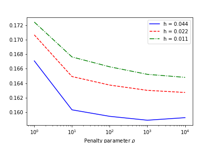
In Figure 4 the behavior of the quantity $\|\lambda_{k}^{a}(u)\|^{2}_{L^{2}(\Omega)}+\|\lambda_{k}^{b}(u)\|^{2}_{L^{2}(\Omega)}$ is plotted along the iterations, i.e., for increasing $\rho_{k}$ , for different discretization levels. In Figure 5, the respective solution plots are shown. While the multipliers seem to be bounded for one example, their norm grows with $\rho$ (and thus with $\epsilon$ ) for the other example. Clearly, more research has to be done to develop necessary and sufficient conditions for the boundedness of the multipliers.

Acknowledgement

The authors are grateful to Gerd Wachsmuth for an inspiring discussion that led to an improvement of Theorem 3.12 and subsequent results.

References

[1] R. Acar and C. R. Vogel. Analysis of bounded variation penalty methods for ill-posed problems. Inverse Problems, 10(6):1217–1229, 1994.
[2] H. Attouch, G. Buttazzo, and G. Michaille. Variational analysis in Sobolev and BV spaces, volume 6 of MPS/SIAM Series on Optimization. Society for Industrial and Applied Mathematics (SIAM), Philadelphia, PA; Mathematical Programming Society (MPS), Philadelphia, PA, 2006. Applications to PDEs and optimization.
[3] S. Bartels. Total variation minimization with finite elements: convergence and iterative solution. SIAM J. Numer. Anal., 50(3):1162–1180, 2012.
[4] S. Bartels and M. Milicevic. Iterative finite element solution of a constrained total variation regularized model problem. Discrete Contin. Dyn. Syst. Ser. S, 10(6):1207–1232, 2017.
[5] E. Casas, K. Kunisch, and C. Pola. Regularization by functions of bounded variation and applications to image enhancement. Appl. Math. Optim., 40(2):229–257, 1999.
[6] E. Casas, R. Herzog, and G. Wachsmuth. Optimality conditions and error analysis of semilinear elliptic control problems with $L^{1}$ cost functional. SIAM J. Optim., 22(3):795–820, 2012.
[7] E. Casas, F. Kruse, and K. Kunisch. Optimal control of semilinear parabolic equations by BV-functions. SIAM J. Control Optim., 55(3):1752–1788, 2017.
[8] E. Casas and K. Kunisch. Analysis of optimal control problems of semilinear elliptic equations by BV-functions. Set-Valued Var. Anal., 27(2):355–379, 2019.
[9] A. Chambolle, V. Caselles, D. Cremers, M. Novaga, and T. Pock. An introduction to total variation for image analysis. In Theoretical foundations and numerical methods for sparse recovery, volume 9 of Radon Ser. Comput. Appl. Math., pages 263–340. Walter de Gruyter, Berlin, 2010.
[10] T. F. Chan, S. Esedoglu, F. E. Park, and A. M. Yip. Total variation image restoration: Overview and recent developments. In N. Paragios, Y. Chen, and O. D. Faugeras, editors, Handbook of Mathematical Models in Computer Vision, pages 17–31. Springer, 2006.
[11] C. Clason and K. Kunisch. A duality-based approach to elliptic control problems in non-reflexive Banach spaces. ESAIM Control Optim. Calc. Var., 17(1):243–266, 2011.
[12] D. Hafemeyer and F. Mannel. A path-following inexact Newton method for optimal control in BV, 2020.
[13] D. Kinderlehrer and G. Stampacchia. An introduction to variational inequalities and their applications, volume 88 of Pure and Applied Mathematics. Academic Press, Inc. [Harcourt Brace Jovanovich, Publishers], New York-London, 1980.
[14] K. Kunisch and D. Wachsmuth. Sufficient optimality conditions and semi-smooth Newton methods for optimal control of stationary variational inequalities. ESAIM Control Optim. Calc. Var., 18(2):520–547, 2012.
[15] H. P. Langtangen and A. Logg. Solving PDEs in Python, volume 3 of Simula SpringerBriefs on Computing. Springer, Cham, 2016. The FEniCS tutorial I.
[16] M. Milicevic. Finite Element Discretization and Iterative Solution of Total Variation Regularized Minimization Problems and Application to the Simulation of Rate-Independent Damage Evolutions. PhD thesis, Universität Freiburg, 2018.
[17] L. I. Rudin, S. Osher, and E. Fatemi. Nonlinear total variation based noise removal algorithms. Phys. D, 60(1-4):259–268, 1992. Experimental mathematics: computational issues in nonlinear science (Los Alamos, NM, 1991).
[18] C. Scheven and T. Schmidt. On the dual formulation of obstacle problems for the total variation and the area functional. Ann. Inst. H. Poincaré Anal. Non Linéaire, 35(5):1175–1207, 2018.
[19] A. Schiela and D. Wachsmuth. Convergence analysis of smoothing methods for optimal control of stationary variational inequalities with control constraints. ESAIM Math. Model. Numer. Anal., 47(3):771–787, 2013.
[20] F. Tröltzsch. Optimal control of partial differential equations, volume 112 of Graduate Studies in Mathematics. American Mathematical Society, Providence, RI, 2010. Theory, methods and applications, Translated from the 2005 German original by Jürgen Sprekels.

	$\displaystyle\|(\lambda^{b}_{\rho_{k}}(u_{k}),\,u_{k}-u_{b})\|$	$\displaystyle\leq\int_{\Omega}{\max}_{\rho_{k}}(\rho_{k}(u_{k}-u_{b}))\|u_{k}-u_{b}\|\,\mathrm{d}x$
		$\displaystyle\leq\int_{\Omega}\left(\rho_{k}(u_{k}-u_{b})_{+}+\frac{1}{2\rho_{k}}\right)\|u_{k}-u_{b}\|\,\mathrm{d}x$
		$\displaystyle=\rho_{k}\int_{\Omega}(u_{k}-u_{b})_{+}(u_{k}-u_{b})\,\mathrm{d}x+\int_{\Omega}\frac{1}{2\rho_{k}}\|u_{k}-u_{b}\|\,\mathrm{d}x$
		$\displaystyle=\rho_{k}\\|(u_{k}-u_{b})_{+}\\|_{L^{2}(\Omega)}^{2}+\frac{1}{2\rho_{k}}\\|u_{k}-u_{b}\\|_{L^{1}(\Omega)}.$

A penalty scheme to solve constrained non-convex optimization problems in B​V​(Ω)BV(\Omega)

1 Introduction

2 Preliminaries and Background

Proposition 2.1.

Proof.

Notation.

2.1 Standing assumption

Assumption A.

Example 2.2.

Example 2.3.

2.2 Existence of solutions of (1.1)

Theorem 2.4.

Proof.

2.3 Necessary optimality conditions

Theorem 2.5.

Proof.

3 Regularization scheme

Lemma 3.1.

Proof.

Corollary 3.2.

Algorithm 3.3.

3.1 A-priori bounds

Lemma 3.4.

Proof.

Lemma 3.5.

Proof.

Corollary 3.6.

Proof.

Corollary 3.7.

Proof.

Lemma 3.8.

Proof.

3.2 Preliminary convergence results

Lemma 3.9.

Proof.

Theorem 3.10.

Proof.

Lemma 3.11.

Proof.

Theorem 3.12.

Proof.

3.3 Convergence of iterates

Lemma 3.13.

Proof.

Lemma 3.14.

Proof.

Theorem 3.15.

Proof.

Theorem 3.16.

Proof.

3.4 Global solutions

Theorem 3.17.

Proof.

4 Optimality condition by regularization

Corollary 4.1.

Proof.

Lemma 4.2.

Proof.

Theorem 4.3.

Proof.

5 Numerical tests

5.1 Globalized Newton Method for the subproblems

Algorithm 5.1 (Global Newton method).

5.2 Example 1: linear elliptic PDE

5.3 Example 2: Semilinear elliptic optimal control problem

5.4 Experiments with non-constant constraints

Acknowledgement

References

A penalty scheme to solve constrained non-convex optimization problems in $BV(\Omega)$