A Parameter Setting Heuristic for the Quantum Alternating Operator Ansatz

The amplitude $q_{\ell}(x)$ of a bitstring $x$ at step $\ell$ induced by applying a layer of QAOA with parameters $(\gamma,\beta)$ to a QAOA state with $\ell-1$ layers can be expressed succinctly as [39]

where $d_{xy}$ is the Hamming distance between bitstrings $x$ and $y$, $\cos\beta^{n-d_{xy}}(-i\sin\beta)^{d_{xy}}=\bra{x}e^{-i\beta B}\ket{y}$ are the mixing operator matrix elements, $c_{y}$ is the cost of bitstring $y$, and the sum is over all $2^{n}$ bitstrings $y$ in the computational basis.

Grouping the terms in Eq. (2), we can rewrite the sum as

where the sum over $d$ runs from $[0,n]$ and the sum over $c$ runs over the set of unique costs allowed by the cost function, which we describe in Sec. II.2. If it is the case that the amplitudes $q_{\ell-1}(x)$ of all bitstrings with cost $c^{\prime}$ are identical, then we can substitute $q(x)$ with $Q(c(x))$ for all $x$. This is exactly Perfect Homogeneity as described in Def. 1. For the rest of this text we use this upper case $Q(c(x))$ to distinguish a function of cost $c=c(x)$ rather than the bitstring $x$ itself. This substitution yields

where $n(x;d,c)$ represents the number of bitstrings with cost $c$ that are of Hamming distance $d$ from $x$. We note that for this equation, and all following equations, this evolution is no longer restricted to unitary evolution. As such, the values $q$ and $Q$ no longer represent strictly quantum amplitudes, but rather track an object that is an analogue to the quantum amplitude. We now introduce the major modification to the sum-of-paths equations. For this, we replace each distribution $n(x;d,c)$ with some distribution $N(c^{\prime};d,c)$ where $c_{x}=c^{\prime}$, where we again adopt the upper case $N$ to distinguish a new distribution that solely depends on the cost of the bitstring. This distribution will generally differ from the original, but in this work we exhibit cases where $N(c^{\prime};d,c)$ is efficiently computable and can adequately replaces $n(x;d,c)$ for the purpose of parameter setting. These cases are discussed in Sec. III and the effectiveness of the replacement is numerically explored in Sec. V.

Using $N(c^{\prime};d,c)$ distributions to replace $n(x;d,c)$, then, we can further rewrite the sum as

where $Q_{\ell}(c^{\prime})$ is used to make explicit that the substitutions yield an expression for $q_{\ell}(x)$ that depends solely on the cost $c^{\prime}$ of bitstring $x$. This leads to a crucial point for our analysis: if we start in a state observing Perfect Homogeneity, and if the distributions $n(x;d,c)$ can be replaced by distributions $N(c^{\prime};d,c)$, which solely depend on the cost $c^{\prime}$ of $x$, then subsequent layers retain the Perfect Homogeneity of the state, yielding analogues of amplitudes $Q(c^{\prime})$. Thus, Eq. (5) is a recursive equation yielding Perfectly Homogeneous analogues of quantum states, which we label the Classical Homogeneous Proxy for QAOA. We here note that importantly, the proxy will not return the analogue of amplitude of some bitstring $x$, but rather the analogue of amplitude of bitstrings with cost $c^{\prime}$, as implicit knowledge of which bitstrings $x$ have cost $c^{\prime}$ would solve the underlying objective function. In Sec. V we argue that there are cases where these analogue of amplitudes $Q(c^{\prime})$ are close to all $q(x)$ with $c_{x}=c^{\prime}$.

In order to evaluate Eq. (5), we note that the set of costs to which indices $c$ and $c^{\prime}$ belong must be defined. Ideally, this set represents exactly the unique objective function values allowed by the underlying cost function. For optimization problems, however, this set is unknown, and is precisely what we would like to solve. Instead, we can form a reasonable estimate by determining upper and lower bounds on the cost function value, as well as by excluding energies which can be efficiently determined to be excluded by the cost function. In this work we denote this estimated set of unique costs as $\mathcal{C}$. As an example, for CSPs with binary valued clauses, the cost function counts the number of satisfied clauses, trivially yielding $\mathcal{C}=\{0,1,...,m\}$, where $m$ is the number of clauses. The set $\mathcal{C}$ also allows us to define the initial state $Q_{0}(c^{\prime})$ for the algorithm. QAOA typically begins with a uniform superposition over all bitstrings $x$, such that $q_{0}(x)=\frac{1}{\sqrt{2^{n}}}$ for all $x$. Thus we can set $Q_{0}(c^{\prime})=\frac{1}{\sqrt{2^{n}}}$ for all $c^{\prime}$ in $\mathcal{C}$.

While Eq. (5) yields analogues of amplitudes $Q_{\ell}(c^{\prime})$, one may also wish to use the Classical Homogeneous Proxy for QAOA to return an estimate of expected value of the cost function. This requires computing a distribution $P(c^{\prime})$ for all $c^{\prime}$ in $\mathcal{C}$, representing the probability a randomly chosen bitstring has cost $c^{\prime}$, averaged over the entire class. Much like in the case of computing $\mathcal{C}$, this computation is approximate, as a perfect computation of this distribution would solve the underlying objective function. Examples of estimations of $P(c^{\prime})$ are shown in Sec. III. In order to compute our estimate of expected value of the cost, then, we simply sum over costs $c^{\prime}$, weighting by the expected number of bitstrings with cost $c^{\prime}$ ($2^{n}P(c^{\prime})$) and the squared analogue to the amplitude $|Q_{\ell}(c^{\prime})|^{2}$,

with the tilde indicating the use of the proxy and that this is no longer a strictly normalized quantum expectation value. This is exactly the equation we use for the homogeneous parameter objective function as described in the introduction. Note that $P(c^{\prime})$ does not give a bona fide probability distribution unless it is re-normalized by dividing by $\sum_{c^{\prime}}2^{n}P(c^{\prime})|Q_{\ell}(c^{\prime})|^{2}$ at each step; nevertheless we have found these factors remain close to unity for the parameter setting experiments considered below and so we neglect them going forward, which yields further computational savings. It is straightforward to introduce these factors into Eq. 6 if desired in other applications.

The set $\mathcal{C}$ and estimate to cost $\widetilde{\braket{C}}$ are critically determined by the class of problems one is working with. Examples of these values for a sample of classes is given in Sec. III.

Formalizing the results in this section, we present Algorithm 1, which describes how given QAOA parameters $p,\vec{\gamma},\vec{\beta}$ a set of possible costs $\mathcal{C}$, and assumed cost distribution $N(c^{\prime};d,c)$ we can compute the Classical Homogeneous Proxy for QAOA using Eq. (5) and Eq. 6.

Time Complexity: Given $N(c^{\prime};d,c)$ as well as $Q_{\ell-1}(c^{\prime})$ for all $c^{\prime}$ in $\mathcal{C}$, the calculation of each amplitude $Q_{\ell}(c^{\prime})$ using Eq. (5) is $\mathcal{O}(n|\mathcal{C}|)$. Thus, the calculation of all $|\mathcal{C}|$ amplitudes $Q_{\ell}(c^{\prime})$ is $\mathcal{O}(n|\mathcal{C}|^{2})$. Computing all $Q_{p}(c^{\prime})$ elements then is $\mathcal{O}(np|\mathcal{C}|^{2})$. If desired, the evaluation of the cost function, given in Eq. (6), involves a sum over $\mathcal{C}$ elements, thus is $\mathcal{O}(|\mathcal{C}|)$.

Thus, if $|\mathcal{C}|$ is $O(\mathrm{poly}(n))$, then Algorithm 1 is efficient. Indeed, we show such a case in the following section, demonstrating how to calculate the necessary pre-computations of $\mathcal{C}$, as well as $N(c^{\prime};d,c)$ and $P(c^{\prime})$ for all $c^{\prime}$ in $\mathcal{C}$.

We first analyze MaxCut on Erdős-Rényi random graphs $\mathcal{G}(n,p_{e})$. In this model, a graph $G$ is generated by scanning over all possible $\binom{n}{2}$ edges in an $n$ node graph, and including each edge with independent probability $p_{e}$. The MaxCut problem on $G$ is to partition the $n$ nodes into two sets such that the number of cut edges crossing the partition is maximized. With respect to the class $\mathcal{G}(n,p_{e})$ of graphs the cost function to be maximized over configurations $x$ is

where $e_{ij}$ are independent binary random variables that take on value $0$ with probability $1-p_{e}$ and $1$ with probability $p_{e}$. We use this cost function to evaluate the relevant distributions in Eq. (11). We start by noting for a fixed graph $G$ with $m$ edges we have $0\leq c(x)\leq m$, and the expected number of edges $\mathbb{E}[m]$ in graphs drawn from $\mathcal{G}(n,p_{e})$ is $p_{e}\binom{n}{2}$, with a standard deviation proportional to to the square root of this value as determined by the binomial distribution. Hence, as $n$ becomes large the expected number of edges concentrates to $p_{e}\binom{n}{2}$, and so for simplicity in the remainder of this work we set $\mathcal{C}=\{0,1,\dots,\lceil\mathbb{E}[m]\rceil\}$. Note that in practice, to accommodate the possibility of a given instance with maximum cut greater than this quantity, one may increase $\mathcal{C}$ by several standard deviations as desired.

We can then easily calculate $P(c^{\prime})$, the probability a random bitstring has cost $c^{\prime}$ for Eq. (12). For a bitstring drawn uniformly at random, the probability of satisfying any given clause $x_{i}\oplus x_{j}$ is $1/2$, as there are two satisfying assignments ($01$ and $10$), and two non-satisfying assignments ($00$ and $11$). Thus, the probability $P(c^{\prime})$ also follows a binomial distribution and is simply

We can then calculate $P_{\textnormal{both}}$, $P_{\textnormal{one}}$ and $P_{\textnormal{neither}}$, where we show all three for didactic purposes (since $P_{\textnormal{both}}+2P_{\textnormal{one}}+P_{\textnormal{neither}}=1$). To see this, consider two randomly chosen bitstrings $y$ and $z$, separated by Hamming distance $d$. We note that there are $(n-d)$ bits in common between $y$ and $z$ and $d$ bits different. Thus $y_{i}\oplus y_{j}=z_{i}\oplus z_{j}$ requires that either both $i$ and $j$ are from the set of $(n-d)$ same bits or the set of $d$ different bits, which has probability

From this expression, we can easily see that $P_{\textnormal{both}}=P_{\textnormal{neither}}=\frac{1}{2}P_{\textnormal{same}}$. Since $P_{\textnormal{same}}$ represents the probability that $y_{i}\oplus y_{j}=z_{i}\oplus z_{j}$, for a random clause and a random bitstring, the probability that $y_{i}\oplus y_{j}=1$ is $1/2$ and the same is true for $y_{i}\oplus y_{j}=0$ by symmetry. Thus we have

For completion, we can calculate $P_{\textnormal{one}}$, which is $(1-P_{\textnormal{same}}-P_{\textnormal{both}})/2$ as shown in Sec. II.1. For this term we need $y_{i}\oplus y_{j}\neq z_{i}\oplus z_{j}$, which can be accomplished if one of $i$ or $j$ is chosen from the $(n-d)$ bits in common and the other is chosen from the $d$ differing bits. This probability is

Thus, $P_{\textnormal{one}}$, which is the probability of specifically $y$ satisfying and $z$ not satisfying (or vice versa) is half of $P_{\textnormal{dif}}$, so

Using these quantities $N(c^{\prime};d,c)$ is then obtained from Eq. 11.

We next consider the MaxE3Lin2 problem which generalizes MaxCut. QAOA for MaxE3Lin2 was analyzed by Farhi et al. [2], who showed an advantage over classical approximation algorithms, only to inspire better classical approaches [40, 41]. The analogous random class of MaxE3Lin2 problems has cost function

where the $z_{abc}$, $,d_{abc}$ are independent random variables with equal probability of being $0$ or $1$.

Using Eq. (18) we can again calculate the relevant probability distributions. First note that a random bitstring $x$ will satisfy a individual clause (i.e. term in the sum) with probability $1/2$, as $(x_{a}+x_{b}+x_{c})\mod 2$ has an equal probability to be $0$ or $1$. Thus,

using the binomial distribution. Then we note that, as in Sec. III.1, the probability of $(y_{a}+y_{b}+y_{c})\mod 2=(z_{a}+z_{b}+z_{c})\mod 2$ for two random bitstrings with $d(x,y)=d$ is given by

since the value of $(x_{a}+x_{b}+x_{c})\mod 2$ is preserved if none or two of $x_{a},x_{b},x_{c}$ are flipped, which is satisfied if $a,b,c$ are all from the $n-d$ identical bits, or two of $a,b,c$ are chosen from the $d$ differing bits. Thus, we can easily compute $P_{\textnormal{both}}=P_{\textnormal{neither}}=P_{\textnormal{same}}/2$, since there is an equal chance $(y_{a}+y_{b}+y_{c})\mod 2=(z_{a}+z_{b}+z_{c})\mod 2=0/1$. $P_{\textnormal{one}}$ can then be calculated by a similar argument or by taking $P_{\textnormal{one}}=(1-P_{\textnormal{both}}-P_{\textnormal{neither}})/2$. We note that the probability distributions calculated here are exactly equivalent to those for the Max-3-XOR problem, where all $z_{abc}$ in Eq. (18) are taken to be $1$.

The MaxEkLin2 problem is a further generalization for each fixed for fixed $k$ of MaxE3Lin2, where we replace the $a,b,c$ with $a_{1},...,a_{k}$ in the cost function and the sum is taken over hyperedges of size $k$. This class of problems was previously studied for QAOA in [42, 43]. For each $k$, $P(c^{\prime})$ is the same as for MaxE3Lin2 above. However, $P_{\textnormal{same}}$ is given by

where the terms in the sum represent all possible ways to choose an even number of bits to flip from the $k$ bits in the clause out of $d$ total bits. Then, again, we have again $P_{\textnormal{both}}=P_{\textnormal{neither}}=P_{\textnormal{same}}/2$ and $P_{\textnormal{one}}=(1-P_{\textnormal{both}}-P_{\textnormal{neither}})/2$. A similar calculation for the Max-k-XOR problem again yields identical probability distributions.

The case of random k-SAT is analyzed by Hogg in [3]. This cost function is defined as the sum over $m$ clauses of a logical OR of $k$ variables randomly drawn from a set of $n$ variables, each of which may be negated. In the notation used in this paper, the distributions of interest are

For these experiments, we first choose ten $\mathcal{G}(10,1/3)$ Erdős-Rényi model graphs, and calculate the $n(x;d,c)$ for all bitstrings $x$ in $\{0,1\}^{n}$, all d in $[0,n]$ and all $c$ in $[0,m]$, with $m$ being an upper bound on the maximum cost (here we use $p_{e}\binom{n}{2}$, as described in Sec. III.1, in this case $m=15$). For each cost $c^{\prime}$, we consider $n(x;d,c)$ for all states $x$ with cost $c^{\prime}$ across all $10$ graphs. In order to evaluate the viability of replacing $n(x;d,c)$ with $N(c^{\prime};d,c)$, we present the following intuition: the better that $N(c^{\prime};d,c)$ estimates the average of $n(x;d,c)$ over all $x$ with $c(x)=c^{\prime}$, and the less that $n(x;d,c)$ deviates over $x$ with $c(x)=c^{\prime}$, the better $N(c^{\prime};d,c)$ should estimate $n(x;d,c)$ for all $x$ with $c(x)=c^{\prime}$. We thus aim to numerically demonstrate the extent to which both the analytically derived $N(c^{\prime};d,c)$ estimate the average $n(x;d,c)$ and to which $n(x;d,c)$ deviates from its average. We first demonstrate the latter. To do this, we take the element-wise averages of these distributions. This average is one way of computing the distributions $N(c^{\prime};d,c)$, as described in Sec. II.1. We also take the element-wise standard deviations of these distributions. In Fig. 2 we display the element-wise ratio of standard deviation to mean of these distributions for $c^{\prime}=7$, chosen because $P(c^{\prime})$ is maximal near $7$, such that this term has large weight in Eq. (5).

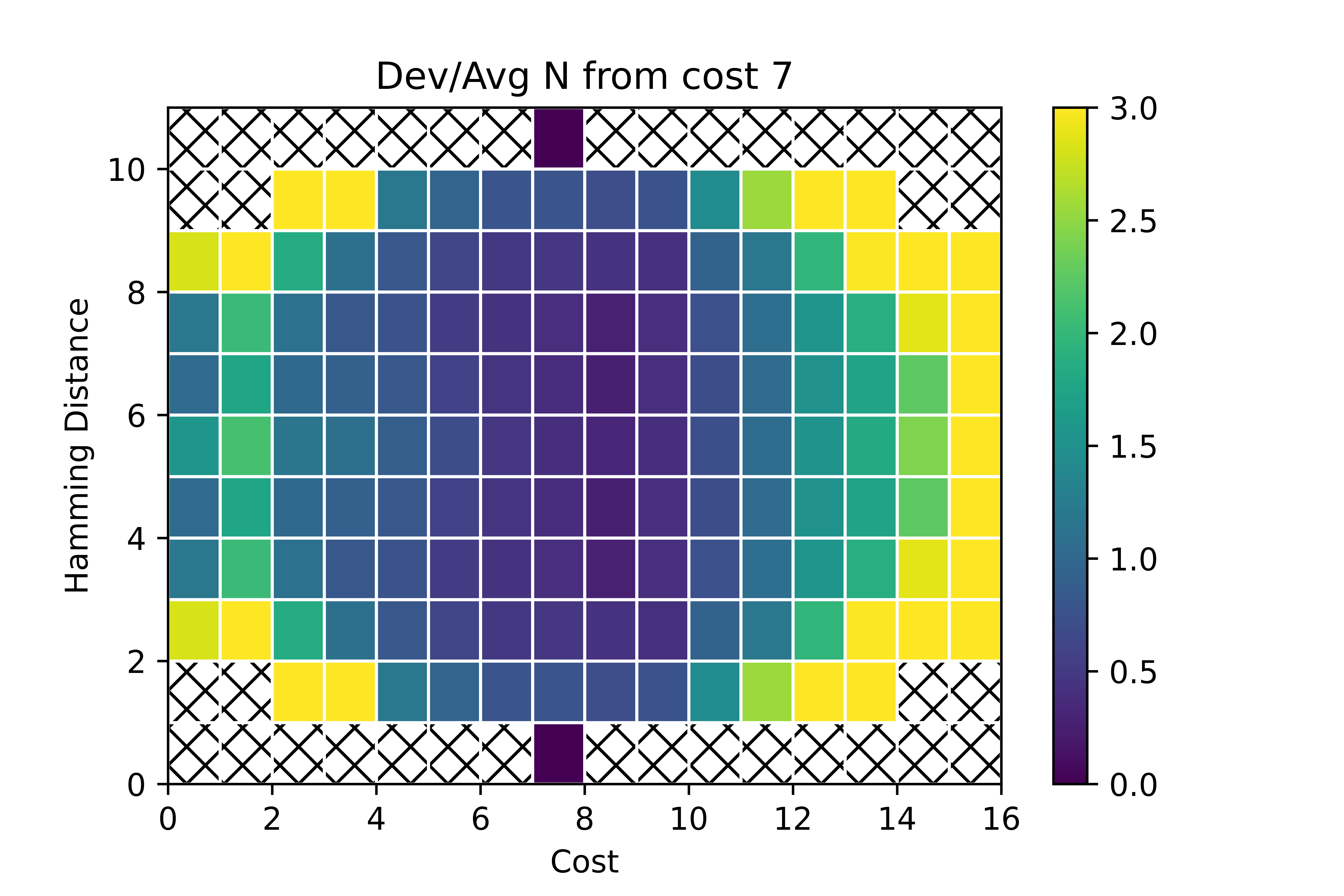
From the figure, we see that for costs near $m/2$ ($7.5$) and distances near $n/2$ ($5$), there is minimal deviation in the $N(c^{\prime};d,c)$ distributions among multiple instances of Erdős-Rényi model graphs and multiple bitstrings $x$ with cost $c^{\prime}$. We note that the relative deviation is highest at the edges of the plot, where $d\rightarrow 0$, $d\rightarrow n$, $c\rightarrow c_{min}$, and $c\rightarrow c_{max}$. We note, however, that at these points, the expected value of $n(x;d,c)$ is smaller, such that the contribution of these deviations to the sum in Eq. (4) is less than those with distance and cost near the center of the distribution. As an example, there are $\binom{10}{5}=252$ bitstrings at distance $5$ from a given bitstring $x$, as opposed to $\binom{10}{1}=10$ bitstrings at distance $1$. A similar argument can be made using the values of $P(c^{\prime})$ derived in Sec. III. This numerical evidence thus suggests that replacing $n(x;d,c)$ with $N(c^{\prime};d,c)$ determined via an averaging over all $x$ with cost $c^{\prime}$ over multiple instances may introduce deviations from Eq. (5) precisely in cases that contribute to less Eq. (2), allowing for near-homogeneous evolution.

This result provides evidence that the deviation in $n(x;d,c)$ is small for the “bulk” of contributions to the sum in Eq. (2), such that we can replace $n(x;d,c)$ with $N(c^{\prime};d,c)$, the average over $x$ with $c(x)=c^{\prime}$ for the entire class of problems. We then would like to understand how the analytically derived expressions for $N(c^{\prime};d,c)$ in Sec. III estimate these averaged distributions. We perform the comparison of $N(c^{\prime};d,c)$ computed by averaging and the methods in Sec. III for MaxCut on Erdős-Rényi model graphs in Fig. 3, showing the Pearson correlation coefficient between the two distributions for each $c^{\prime}$ in $[0,m]$. We likewise display $P(c^{\prime})$, in order to elucidate the dominant distributions in the sum of Eq. (5).

From the figure we see that for dominant terms (with high $P(c^{\prime})$), the two distributions align well visually, corresponding to a high correlation coefficient. For less important terms, the analytical distributions do not match the average over many instances, but the effect of this mismatch may be reduced due to the lesser weight on these terms as determined by $P(c^{\prime})$ in the sums of equation Eq. (5).

Combined, Figs. 2 and 3 show that for dominant terms, there is little deviation in $n(x;d,c)$ distributions from their average $N(c^{\prime};d,c)$, and the analytically computed distributions match these average distributions well. Thus, they together indicate that the analytical methods for calculating $N(c^{\prime};d,c)$ should approximate $n(x;d,c)$ with $c(x)=c^{\prime}$ for terms that dominate the sum in Eq. (5).

To further investigate the viability of the Classical Homogeneous Proxy for QAOA, we perform numerical simulations of the proxy on MaxCut on Erdős-Rényi graphs $\mathcal{G}(10,.5)$, and display the squared overlap between classical full statevector simulation and the proxy as a function of $p$ for various parameter schedules motivated by QAOA literature. For this analysis, we choose linear ramp parameter schedules, inspired by quantum annealing. In particular, we fix a starting and ending point for $\vec{\gamma}$ and $\vec{\beta}$, which is kept constant regardless of $p$, and the schedule is defined as

for each layer ${\ell}$. Given these linear ramp schedules, the squared overlaps between the replace and original quantities are calculated as follows. First, statevector simulation was performed using HybridQ, an open-source package for large-scale quantum circuit simulation [44]. Next, the $N(c^{\prime};d,c)$ distributions are computed according to Eq. III. Then, for the purposes of comparison, we compute the proxy slightly differently from above, by starting with the uniform superposition over all $2^{n}$ bitstrings and simply plugging in $N(c(x);d,c)$ for all $n(x;d,c)$ in Eq. (4), keeping all $2^{n}$ amplitudes $q^{\ell}(x)$ at each step $\ell$. This allows us to compute the overlap between the proxy and true state using standard quantum state overlap, although we lose the gain in complexity from performing the proxy on only the set of unique costs, as we are working with $2^{n}$ bitstrings rather than $|\mathcal{C}|$ costs. Then, using this method, we plot the squared overlaps between the replace and original quantities as a function of $p$ with varying values of $\gamma_{1}$ and $\gamma_{f}$ in Fig. 4.

From the figure, we can see that the overlap gradually decreases as the number of QAOA layers increases. However, the decline is less dramatic when $\gamma_{1}$ and $\gamma_{f}$ are lower in magnitude. Thus, we see that as we move towards the $\gamma\ll 1$ regime for these problems (or, more precisely $\gamma\ll\|C\|$ [39]), the true QAOA state remains closer to the proxy even as the algorithm progresses, as remarked in Sec II. We stress that this behavior is empirical and the numerics are limited to the MaxCut examples analyzed presently. This behavior does however align with the analytical fact mentioned in Sec. II that to first order in $\gamma$, QAOA states are Perfectly Homogeneous for strictly k-local Hamiltonians.

In order to provide an explicit illustrative example for the efficacy of the Homogeneous Heuristic for Parameter Setting in Alg. 3, we depict the both the typical and homogeneous parameter objective function as a function of $\gamma_{3}$ and $\beta_{3}$ for a randomly drawn $\mathcal{G}(8,1/2)$ graph and QAOA with $p=3$. In this example, our aim is to visualize similarities between the two parameter objective functions rather than to exhaustively find optimal parameters for the graph. As such, we borrow $\gamma_{1}$, $\gamma_{2}$, $\beta_{1}$ and $\beta_{2}$, optimized from a $20$ node instance in Sec. VI.1. These landscapes are shown in Fig. 5.

It is visually clear that the two landscapes have significant differences. For the typical parameter objective function, there exists a clearly defined, Gaussian-like peak (yellow) and valley (blue). For the homogeneous parameter objective function, there exists a similarly-located peak, albeit vertically compressed, and the corresponding valley comprises almost the entire rest of the landscape. However, we can see that in the small $\gamma$ regime in particular, the landscapes qualitatively look very similar. This behavior is suggested by Fig. 4, where we see quantitatively that the extent to which the Classical Homogeneous Proxy for QAOA overlaps with the true QAOA evolution grows as $\gamma$ decreases. Additionally, as seen in previous studies of QAOA parameters [13, 14, 11, 10], optimal values of $\gamma$ tend to remain relatively small (exact values are not described as they depend on $n$, $p$, and the cost function being used), especially at the beginning of the algorithm. This suggests that, while the homogeneous and typical parameter objective functions may deviate significantly in general, they maintain significant correlations in relevant parameter regimes, specifically those which are near the maximum in the landscape. Indeed, for the task of parameter setting, we expect qualitative feature mapping of the landscape to be much more important than a precise matching of objective function values.

It is also worthwhile to consider the difference in computational resources needed to produce the two plots. For the typical parameter objective function, in order to classically evaluate the evolution of the algorithm in each cell of the presented 30 by 30 landscapes, we perform full statevector simulation. Farhi et al. show in [2], that in order to compute Pauli observable expectation values for the typical parameter objective function, one only needs to include qubits that are within the reverse causal cone generated by the qubits involved in the observable and the quantum circuit implementing QAOA. However, for the example analyzed here, at $p=3$, this reverse causal cone includes all $8$ qubits for each observable, so in order to classically compute the evolution, we perform a full-state simulation. Thus, deriving evolution of the proxy took roughly one-fiftieth of the time required for simulating full QAOA. We note that it is possible to efficiently evaluate each cell on an actual quantum computer, and that if one only wants expectation values given parameters rather than the full state evolution, there are more efficient classical methods (e.g. [2, 31]). Current difficulties for this approach, however include noise resulting both from finite sampling error as well as the effects of imperfect quantum hardware.

Here we present results of the Homogeneous Heuristic for Parameter Setting, as well as comparisons to the transfer of parameters method outlined in Lotshaw et al. [10], implemented using the QAOAKit software package [11]. Lotshaw et al. show that using one set of median (over the entire dataset at a given $n$ and $p$) parameters performs similarly to optimized parameters for each instance. Thus, we directly pull the obtained parameters from QAOAKit, which first calculates optimal parameters for all connected non-isomorphic graphs up to size $9$ at $p=1$,$2$, and $3$. For each $p$, the median over all parameters is calculated, and these median parameters are directly applied to ten Erdős-Rényi graphs from $\mathcal{G}(20,1/2)$, yielding average and standard deviation of expectation values for these median parameters over the ten graphs. To compare with these transferred parameters, we display the approximation ratio achieved by parameters that are optimized with the heuristic, as described in Sec. IV, over the same ten graphs. Here the approximation ratio is defined as follows,

i.e., the expected cost value returned by true QAOA, divided by the true optimal value $c_{opt}$, as determined via brute force search over all $2^{n}$ bitstrings. For this experiment, as well as all experiments below, the state throughout the algorithm and $\braket{C}$ are computed via full statevector simulation, even for parameters returned via the heuristic. The comparison between the heuristic and parameter transfer is shown in Fig. 6.

As we can see in Fig. 6, for low depth, the heuristic performs comparably well to parameter transfer. On an instance-by-instance basis, the approximation ratio achieved by homogeneous parameter setting minus that achieved by parameter transfer was $-.0037\pm.0062$, $.0164\pm.0148$, and $.0097\pm.0183$ for $p=1$, $2$, and $3$, respectively. We do not see statistically significant differences between the two methods for any three of the depths analyzed, although the average performance of the heuristic is slightly higher in the latter two cases. This numerical evidence indicates that the method is competitive. Furthermore, the optimal parameters in the transfer case require the optimization of smaller QAOA instances, which clearly may incur some tradeoff between the size of problem one wishes to train parameters on versus the accuracy of the parameter transfer onto larger and larger instances. The parameters for comparison were pulled directly from QAOAKit data-tables, so our purpose here is not to provide a full timing comparison between the two methods. However, this demonstrates that our polynomially-scaling heuristic performs comparably with other techniques used in literature.

To elucidate how the Homogeneous Heuristic for Parameter Setting scales with QAOA depth $p$, we further depict box plots of the approximation ratio for a new set of ten Erdős-Rényi graphs $\mathcal{G}(20,.5)$ at $p$ up to $20$. For these experiments, we further restrict to linear ramp parameter schedules as described in Eq. (23), to reduce the number of parameters from $2p$ to $4$. We introduce this re-parameterization because having $2p$ free parameters, even for this relatively moderately sized $p$, results in optimization routines that do not converge in a reasonable time on the device as specified below. The results for these runs are shown in Fig. 7.

From this figure, we see that the heuristic, when implemented with linear ramp schedules, results in monotonic improvement of approximation ratios as $p$ increases. Notably, for this regime of $N=20$, $p=20$, we were not able to find previous works that efficiently returned optimized parameter schedules, even when restricted to linear ramps. Thus, these results demonstrate a regime in which the heuristic is able to return parameters that appear intractable for current devices and strategies, whether quantum, classical, or hybrid.

Numerical details: For our simulations in this section, all calculations (excluding those pulled from the QAOAKit database) were performed using a laptop with Intel i7-10510U CPUs @ 1.80GHz and 16 GB of RAM, with no parallelization utilized. For the $20$ node graphs, all experiments clocked in under $6$ hours, where the longest times were for fully parameterized $p=3$ circuits (6 parameters). Parameters were seeded using linear ramp schedules from [13] and parameter optimization was performed using the standard Broyden–Fletcher–Goldfarb–Shanno algorithm [45] from the SciPy package [46].

References

- [1] Stuart Hadfield, Zhihui Wang, Bryan O’Gorman, Eleanor G. Rieffel, Davide Venturelli, and Rupak Biswas. From the Quantum Approximate Optimization Algorithm to a Quantum Alternating Operator Ansatz. Algorithms, 12(2):34, February 2019. Number: 2 Publisher: Multidisciplinary Digital Publishing Institute.
- [2] Edward Farhi, Jeffrey Goldstone, and Sam Gutmann. A Quantum Approximate Optimization Algorithm. arXiv:1411.4028 [quant-ph], 10(2), November 2014. arXiv: 1411.4028.
- [3] Tad Hogg. Quantum search heuristics. Physical Review A, 61(5):052311, April 2000. Publisher: American Physical Society.
- [4] Tad Hogg and Dmitriy Portnov. Quantum optimization. Information Sciences, 128(3):181–197, October 2000.
- [5] M. Cerezo, Andrew Arrasmith, Ryan Babbush, Simon C. Benjamin, Suguru Endo, Keisuke Fujii, Jarrod R. McClean, Kosuke Mitarai, Xiao Yuan, Lukasz Cincio, and Patrick J. Coles. Variational quantum algorithms. Nature Reviews Physics, 3(9):625–644, September 2021. Number: 9 Publisher: Nature Publishing Group.
- [6] David Wierichs, Christian Gogolin, and Michael Kastoryano. Avoiding local minima in variational quantum eigensolvers with the natural gradient optimizer. Physical Review Research, 2(4):043246, November 2020. arXiv:2004.14666 [quant-ph].
- [7] Jarrod R. McClean, Sergio Boixo, Vadim N. Smelyanskiy, Ryan Babbush, and Hartmut Neven. Barren plateaus in quantum neural network training landscapes. Nature Communications, 9(1):4812, November 2018. Number: 1 Publisher: Nature Publishing Group.
- [8] Martin Larocca, Piotr Czarnik, Kunal Sharma, Gopikrishnan Muraleedharan, Patrick J. Coles, and M. Cerezo. Diagnosing barren plateaus with tools from quantum optimal control. Technical Report arXiv:2105.14377, arXiv, March 2022. arXiv:2105.14377 [quant-ph] type: article.
- [9] Samson Wang, Enrico Fontana, M. Cerezo, Kunal Sharma, Akira Sone, Lukasz Cincio, and Patrick J. Coles. Noise-induced barren plateaus in variational quantum algorithms. Nature Communications, 12(1):6961, November 2021. Number: 1 Publisher: Nature Publishing Group.
- [10] Phillip C. Lotshaw, Travis S. Humble, Rebekah Herrman, James Ostrowski, and George Siopsis. Empirical performance bounds for quantum approximate optimization. arXiv:2102.06813 [physics, physics:quant-ph], February 2021. arXiv: 2102.06813.
- [11] Ruslan Shaydulin, Kunal Marwaha, Jonathan Wurtz, and Phillip C. Lotshaw. QAOAKit: A Toolkit for Reproducible Study, Application, and Verification of the QAOA. arXiv:2110.05555 [quant-ph], November 2021. arXiv: 2110.05555.
- [12] Sami Khairy, Ruslan Shaydulin, Lukasz Cincio, Yuri Alexeev, and Prasanna Balaprakash. Learning to Optimize Variational Quantum Circuits to Solve Combinatorial Problems. Proceedings of the AAAI Conference on Artificial Intelligence, 34(03):2367–2375, April 2020. Number: 03.
- [13] Leo Zhou, Sheng-Tao Wang, Soonwon Choi, Hannes Pichler, and Mikhail D. Lukin. Quantum Approximate Optimization Algorithm: Performance, Mechanism, and Implementation on Near-Term Devices. Physical Review X, page 021067, June 2020. Publisher: American Physical Society.
- [14] Gavin E. Crooks. Performance of the Quantum Approximate Optimization Algorithm on the Maximum Cut Problem. arXiv:1811.08419 [quant-ph], November 2018. arXiv: 1811.08419.
- [15] Ruslan Shaydulin, Ilya Safro, and Jeffrey Larson. Multistart Methods for Quantum Approximate optimization. In 2019 IEEE High Performance Extreme Computing Conference (HPEC), pages 1–8, September 2019. ISSN: 2643-1971.
- [16] Mahabubul Alam, Abdullah Ash-Saki, and Swaroop Ghosh. Accelerating quantum approximate optimization algorithm using machine learning. In 2020 Design, Automation & Test in Europe Conference & Exhibition (DATE), pages 686–689. IEEE, 2020.
- [17] Guillaume Verdon, Michael Broughton, Jarrod R. McClean, Kevin J. Sung, Ryan Babbush, Zhang Jiang, Hartmut Neven, and Masoud Mohseni. Learning to learn with quantum neural networks via classical neural networks. arXiv:1907.05415 [quant-ph], July 2019. arXiv: 1907.05415.
- [18] Max Wilson, Rachel Stromswold, Filip Wudarski, Stuart Hadfield, Norm M. Tubman, and Eleanor G. Rieffel. Optimizing quantum heuristics with meta-learning. Quantum Machine Intelligence, 3(1):13, April 2021.
- [19] Andrea Skolik, Jarrod R McClean, Masoud Mohseni, Patrick van der Smagt, and Martin Leib. Layerwise learning for quantum neural networks. Quantum Machine Intelligence, 3(1):1–11, 2021.
- [20] Javier Rivera-Dean, Patrick Huembeli, Antonio Acín, and Joseph Bowles. Avoiding local minima in variational quantum algorithms with neural networks. arXiv preprint arXiv:2104.02955, 2021.
- [21] Lennart Bittel and Martin Kliesch. Training variational quantum algorithms is NP-hard. Physical Review Letters, 127(12):120502, 2021.
- [22] Michael Streif and Martin Leib. Training the quantum approximate optimization algorithm without access to a quantum processing unit. Quantum Science and Technology, 5(3):034008, May 2020. Publisher: IOP Publishing.
- [23] Ruslan Shaydulin, Stuart Hadfield, Tad Hogg, and Ilya Safro. Classical symmetries and the Quantum Approximate Optimization Algorithm. Quantum Information Processing, 20(11):359, November 2021. arXiv: 2012.04713.
- [24] Lucas T. Brady, Christopher L. Baldwin, Aniruddha Bapat, Yaroslav Kharkov, and Alexey V. Gorshkov. Optimal Protocols in Quantum Annealing and Quantum Approximate Optimization Algorithm Problems. Physical Review Letters, 126(7):070505, February 2021. Publisher: American Physical Society.
- [25] Stefan H. Sack and Maksym Serbyn. Quantum annealing initialization of the quantum approximate optimization algorithm. Quantum, 5:491, July 2021. Publisher: Verein zur Förderung des Open Access Publizierens in den Quantenwissenschaften.
- [26] Jonathan Wurtz and Peter J. Love. Counterdiabaticity and the quantum approximate optimization algorithm. arXiv:2106.15645 [quant-ph], July 2021. arXiv: 2106.15645.
- [27] Fernando G. S. L. Brandao, Michael Broughton, Edward Farhi, Sam Gutmann, and Hartmut Neven. For Fixed Control Parameters the Quantum Approximate Optimization Algorithm’s Objective Function Value Concentrates for Typical Instances. arXiv:1812.04170 [quant-ph], December 2018. arXiv: 1812.04170.
- [28] Xinwei Lee, Yoshiyuki Saito, Dongsheng Cai, and Nobuyoshi Asai. Parameters Fixing Strategy for Quantum Approximate Optimization Algorithm. arXiv:2108.05288 [quant-ph], August 2021. arXiv: 2108.05288.
- [29] Alexey Galda, Xiaoyuan Liu, Danylo Lykov, Yuri Alexeev, and Ilya Safro. Transferability of optimal QAOA parameters between random graphs. arXiv:2106.07531 [quant-ph], June 2021. arXiv: 2106.07531.
- [30] Lucas T Brady, Lucas Kocia, Przemyslaw Bienias, Aniruddha Bapat, Yaroslav Kharkov, and Alexey V Gorshkov. Behavior of analog quantum algorithms. arXiv preprint arXiv:2107.01218, 2021.
- [31] Zhihui Wang, Stuart Hadfield, Zhang Jiang, and Eleanor G. Rieffel. Quantum approximate optimization algorithm for MaxCut: A fermionic view. Physical Review A, 97(2):022304, February 2018. Publisher: American Physical Society.
- [32] Kunal Marwaha. Local classical MAX-CUT algorithm outperforms p=2 QAOA on high-girth regular graphs. Quantum, 5:437, April 2021.
- [33] Panagiotis Kl Barkoutsos, Giacomo Nannicini, Anton Robert, Ivano Tavernelli, and Stefan Woerner. Improving Variational Quantum Optimization using CVaR. Quantum, 4:256, April 2020. arXiv:1907.04769 [quant-ph].
- [34] Li Li, Minjie Fan, Marc Coram, Patrick Riley, and Stefan Leichenauer. Quantum optimization with a novel Gibbs objective function and ansatz architecture search. Physical Review Research, 2(2):023074, April 2020.
- [35] Kevin J Sung, Jiahao Yao, Matthew P Harrigan, Nicholas C Rubin, Zhang Jiang, Lin Lin, Ryan Babbush, and Jarrod R McClean. Using models to improve optimizers for variational quantum algorithms. Quantum Science and Technology, 5(4):044008, 2020.
- [36] Ryan Shaffer, Lucas Kocia, and Mohan Sarovar. Surrogate-based optimization for variational quantum algorithms, April 2022. Number: arXiv:2204.05451 arXiv:2204.05451 [quant-ph].
- [37] Juliane Mueller, Wim Lavrijsen, Costin Iancu, et al. Accelerating noisy VQE optimization with gaussian processes. arXiv preprint arXiv:2204.07331, 2022.
- [38] Pablo Díez-Valle, Diego Porras, and Juan José García-Ripoll. QAOA pseudo-Boltzmann states. arXiv:2201.03358 [quant-ph], March 2022. arXiv: 2201.03358.
- [39] Stuart Hadfield, Tad Hogg, and Eleanor G Rieffel. Analytical framework for quantum alternating operator ansätze. arXiv preprint arXiv:2105.06996, 2021.
- [40] Boaz Barak, Ankur Moitra, Ryan O’Donnell, Prasad Raghavendra, Oded Regev, David Steurer, Luca Trevisan, Aravindan Vijayaraghavan, David Witmer, and John Wright. Beating the random assignment on constraint satisfaction problems of bounded degree. arXiv preprint arXiv:1505.03424, 2015.
- [41] Matthew Hastings. Classical and quantum bounded depth approximation algorithms. Quantum Information and Computation, 19:1116–1140, November 2019.
- [42] Kunal Marwaha and Stuart Hadfield. Bounds on approximating MaxXOR with quantum and classical local algorithms. Quantum, 6:757, 2022.
- [43] Chi-Ning Chou, Peter J Love, Juspreet Singh Sandhu, and Jonathan Shi. Limitations of local quantum algorithms on random Max-k-XOR and beyond. In 49th International Colloquium on Automata, Languages, and Programming (ICALP 2022), 2022.
- [44] Salvatore Mandrà, Jeffrey Marshall, Eleanor G. Rieffel, and Rupak Biswas. HybridQ: A Hybrid Simulator for Quantum Circuits. arXiv:2111.06868 [quant-ph], November 2021. arXiv: 2111.06868.
- [45] R. (Roger) Fletcher. Practical methods of optimization. Chichester ; New York : Wiley, 1987.
- [46] Pauli Virtanen, Ralf Gommers, Travis E. Oliphant, Matt Haberland, Tyler Reddy, David Cournapeau, Evgeni Burovski, Pearu Peterson, Warren Weckesser, Jonathan Bright, Stéfan J. van der Walt, Matthew Brett, Joshua Wilson, K. Jarrod Millman, Nikolay Mayorov, Andrew R. J. Nelson, Eric Jones, Robert Kern, Eric Larson, C. J. Carey, İlhan Polat, Yu Feng, Eric W. Moore, Jake VanderPlas, Denis Laxalde, Josef Perktold, Robert Cimrman, Ian Henriksen, E. A. Quintero, Charles R. Harris, Anne M. Archibald, Antônio H. Ribeiro, Fabian Pedregosa, and Paul van Mulbregt. SciPy 1.0: fundamental algorithms for scientific computing in Python. Nature Methods, 17(3):261–272, March 2020.