A paradigm of spontaneous marginal phase transition at
finite temperature in one-dimensional ladder Ising models
Abstract
The Ising model describes collective behaviors such as phase transitions and critical phenomena in various physical, biological, economical, and social systems. It is well-known that spontaneous phase transition at finite temperature does not exist in the Ising model with short-range interactions in one dimension. Yet, little is known about whether this forbidden phase transition can be approached arbitrarily closely—at fixed finite temperature. To describe such asymptoticity, here I introduce the notion of marginal phase transition (MPT) and use symmetry analysis of the transfer matrix to reveal the existence of spontaneous MPT at fixed finite temperature in one class of one-dimensional Ising models on decorated two-leg ladders, in which is determined solely by on-rung interactions and decorations, while the crossover width is independently, exponentially reduced ( means a genuine phase transition) by on-leg interactions and decorations. These findings establish a simple ideal paradigm for realizing an infinite number of one-dimensional Ising systems with spontaneous MPT, which would be characterized in routine lab measurements as a genuine first-order phase transition with large latent heat thanks to the ultra-narrow (say less than one nano-kelvin), paving a way to push the limit in our understanding of phase transitions and the dynamical actions of frustration arbitrarily close to the forbidden regime.
I Introduction
The textbook Ising model Mattis_book_08_SMMS ; Mattis_book_1985 ; Baxter_book_Ising ; 003_Huang_08_book consists of individuals that have one of two values ( or , e.g., magnetic moments of atomic spins pointing to the up or down direction, open or close in neural networks, yes or no in voting, etc.):
| (1) |
where is the th individual’s value and depicts the bias (e.g., the external magnetic field that favors for ). The individuals interact according to the simple rule that neighbors with like values are rewarded more than those with unlike values (i.e., the ferromagnetic interaction ). Therefore, the society tends to form the order in which all the members have the same value. This tendency is however disturbed by heat, which favors the free choice of the values or disorder. The model was originally proposed for a central question in condensed matter physics, namely whether a spontaneous phase transition (i.e., in the absence of the bias, ) between the high-temperature disordered state and the low-temperature ordered state exists at finite temperature, and in his 1924 doctoral thesis—one century ago—Ernst Ising solved the model exactly for spins localized on a one-dimensional (1D) single chain but found no phase transition Ising1925 . The 2D square-lattice Ising model, which is much harder to be solved exactly, is generally referred to as one of the simplest statistical models to show a spontaneous phase transition at finite temperature Onsager_Ising_2D . Moving from one to two dimension was often described with -leg spin ladders (i.e., coupled parallel chains, which are still 1D; the limit is 2D) Dagotto_science_ladder , and again no phase transition was found for finite Mejdani_Ising_ladder . In fact, the Perron–Frobenius theorem implied the nonexistence of any phase transition in 1D Ising models with short-range interactions Cuesta_1D_PT . The rigorously proved nonexistence of spontaneous phase transition at finite temperature in the 1D Ising model is deeply rooted in symmetry Batista_PRB_05_dimensional-reductions and becomes one of the most quoted limits of human knowledge.
Here, we ask the question of how close the 1D Ising model can get to a phase transition. The ideal answer would be such an ultra-narrow phase crossover that can approach a genuine phase transition arbitrarily closely in a definite way—at a fixed finite temperature and with the crossover width getting narrower and narrower, best exponentially ( means phase transition). We coin the term “marginal phase transition” (MPT) for phase crossovers with the above asymptoticity. Thus, MPT means a pathway in which broad phase crossovers can be readily tuned to be ultra-narrow at the same . Practically speaking, when becomes so narrow (say less than one nano-kelvin), the MPT would be characterized as a genuine phase transition in lab measurements. The quest for MPT will push the limit in our understanding of phase transitions as close as possible to the forbidden regime.
A recent breakthrough relevant to this quest was the discovery of the so-called “pseudo-transition” in a few decorated Ising chains in the presence of the magnetic field 005_Galisova_PRE_15_double-tetrahedral-chain ; 007_Torrico_PRA_16_Ising-XYZ-diamond-chain ; 009_review_Souza_SSC_18_Ising-XYZ-diamond-chain_double-tetrahedral-chain-spin-electron ; 010_Carvalho_JMMM_18_Ising-XYZ-diamond-chain_quantum-entanglement ; 011_Rojas_BJP_20_Ising-Heisenberg-tetrahedral_diamond ; 013_Rojas_PRE_19_previous_4_models ; 014_Rojas_JPC_20_Ising–Heisenberg_spin-1-double-tetrahedral-chain ; 015_Strecka_APPA_20_Ising-diamond-chain ; 015-7_Canova_CzechoslovakJP_04_Ising–Heisenberg_diamond_chain ; 015-8_Canova_JPC_06_Ising–Heisenberg-spin-S-diamond-chain ; 017_Krokhmalskii_PA_21_3-previous-chains_effective_model ; 016_Strecka_book_chapter . For , those 1D Ising chains exhibit the entropy jump and a gigantic peak in specific heat in a narrow temperature region, resembling a first-order phase transition. The construction of the “pseudo-transition” utilized the concept of frustration as follows: The Ising model can also accommodate the opposite rule, namely neighbors with like values are rewarded less than those with unlike values (i.e., antiferromagnetic interaction ). Accordingly, the ordered state has alternating values if such an arrangement can be made, such as ///// on a 1D chain lattice, the checkerboard pattern on the 2D square lattice, etc. (for bipartite lattices, the antiferromagnetic Ising model is equivalent to the ferromagnetic one by the transformation of in one of the two sublattices). However, there are numerous situations where the between-neighbor interactions cannot be simultaneously satisfied. The standard example is a spin triangle (Fig. 2a) where two spins have opposite values, then it is impossible for the third spin to have the opposite value to both of them, leading to the state degeneracy of 2. This phenomenon is called geometrical frustration Balents_nature_frustration ; Miyashita_10_review_frustration . Meanwhile, if the non-degenerate state, where the first two spins couple more strongly to the third spin and satisfactorily have the same value (because of having the opposite value to the third spin), is tuned to be the ground state with slightly lower energy than the aforementioned degenerated state, then a thermal (entropy) driven crossover between them would occur at finite temperature Miyashita_10_review_frustration . This physics of phase crossover is rather generic; what is challenging is how to make the crossover ultra-narrow and asymptotic with fixed . It was significant that the “pseudo-transition” has showcased the existence of ultra-narrow phase crossover in the 1D Ising model for . For , however, the pseudo-transition in those decorated Ising chains is prohibited by spin up-down symmetry 005_Galisova_PRE_15_double-tetrahedral-chain ; 007_Torrico_PRA_16_Ising-XYZ-diamond-chain ; 009_review_Souza_SSC_18_Ising-XYZ-diamond-chain_double-tetrahedral-chain-spin-electron ; 010_Carvalho_JMMM_18_Ising-XYZ-diamond-chain_quantum-entanglement ; 011_Rojas_BJP_20_Ising-Heisenberg-tetrahedral_diamond ; 013_Rojas_PRE_19_previous_4_models ; 014_Rojas_JPC_20_Ising–Heisenberg_spin-1-double-tetrahedral-chain ; 015_Strecka_APPA_20_Ising-diamond-chain ; 015-7_Canova_CzechoslovakJP_04_Ising–Heisenberg_diamond_chain ; 015-8_Canova_JPC_06_Ising–Heisenberg-spin-S-diamond-chain ; 017_Krokhmalskii_PA_21_3-previous-chains_effective_model ; 016_Strecka_book_chapter , suggesting that spontaneous ultra-narrow phase crossover be much harder to realize. We noticed that three cases of zero-field “pseudo-transition” were reported to occur in 2-leg 016_Strecka_book_chapter ; 008_zero-field_Rojas_SSC_16_Ising-Heisenberg_ladder and 3-leg 006_zero-field_Strecka_JMMM_16_Ising-Heisenberg-3-leg-tube ladders; however, the insight into how these few 1D Ising models can escape from the symmetry constraint for the single chain is lacking—as shown below, such symmetry analysis is vital to the generation of an infinite number of zero-field ultra-narrow phase crossover. Above all, the asymptoticity required by MPT has not been addressed in the context of “pseudo-transition,” where even the crossover width was not clearly defined and rigorously expressed in terms of the model parameters 005_Galisova_PRE_15_double-tetrahedral-chain ; 007_Torrico_PRA_16_Ising-XYZ-diamond-chain ; 009_review_Souza_SSC_18_Ising-XYZ-diamond-chain_double-tetrahedral-chain-spin-electron ; 010_Carvalho_JMMM_18_Ising-XYZ-diamond-chain_quantum-entanglement ; 011_Rojas_BJP_20_Ising-Heisenberg-tetrahedral_diamond ; 013_Rojas_PRE_19_previous_4_models ; 014_Rojas_JPC_20_Ising–Heisenberg_spin-1-double-tetrahedral-chain ; 015_Strecka_APPA_20_Ising-diamond-chain ; 015-7_Canova_CzechoslovakJP_04_Ising–Heisenberg_diamond_chain ; 015-8_Canova_JPC_06_Ising–Heisenberg-spin-S-diamond-chain ; 017_Krokhmalskii_PA_21_3-previous-chains_effective_model ; 016_Strecka_book_chapter ; 008_zero-field_Rojas_SSC_16_Ising-Heisenberg_ladder ; 006_zero-field_Strecka_JMMM_16_Ising-Heisenberg-3-leg-tube .
The purpose of this paper is to present the finding of spontaneous MPT (SMPT) in a family of decorated Ising 2-leg ladders with strong frustration Yin_MPT , in which is determined by on-rung interactions, while is independently, exponentially reduced by on-leg interactions for fixed . This establishes a simple ideal paradigm for implementing an infinite number of 1D Ising systems with SMPT Yin_icecreamcone . We further found that the SMPT can be expressed accurately and conveniently by a nonclassical order parameter providing a microscopic description of the abrupt switching between two unconventional long-range orders where the local two-parent-spin correlations are ferromagnetic and antiferromagnetic, respectively. Moreover, we show that the on-leg decoration (which controls ) can be done independently of the on-rung decoration (which controls ), revealing an amazing advantage of this paradigm. Specifically, can be exponentially reduced by increasing the number of on-leg-decorated spins, making it clear that spontaneous phase transition at finite temperature does not exist in the 1D Ising model with a finite number of short-range interactions.
The rest of the paper is organized as follows: Section II heuristically describes the line of thinking and the use of a dimensionality increase and reduction method that utilized symmetry analysis to give rise to the SMPT. For the sake of clarity, Section III details the realization of SMPT in a minimal 1D Ising model by decorating the rungs and the exact solutions about its thermodynamic properties, correlation functions, and nonclassical order parameters. Section IV showcases how to decorate the legs to approach a genuine phase transition at finite temperature arbitrarily closely. Section V addresses some immediate implications of the present work on further fundamental and technological research and development.
II The Method
II.1 SMPT from mimicking the first-order phase transition
The mathematical signature of phase transitions is the non-analyticity of the system’s thermodynamic free energy where denotes temperature. A th-order phase transition means that the th derivative of starts to be discontinuous at the transition. The exactly solved 1D Ising models on both the single chain Mattis_book_08_SMMS ; Mattis_book_1985 ; Baxter_book_Ising ; 003_Huang_08_book and ordinary -leg ladders with Mejdani_Ising_ladder offer examples of analytic free energies.
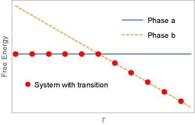
The simplest description of the phase transition phenomenon is the level crossing in the first-order phase transition, such as melting of ice or the boiling of water. As illustrated in Fig. 1a, suppose the free-energy functions of two phases and cross at the critical temperature . Then, the free energy of the system taking the lower value of and is given by
| (2) |
which is nonanalytic at with its first derivative with respect to being discontinuous.
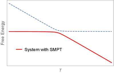
We hypothesize that SMPT can be created by using an analytic function to mimic Eq. (2) and consider here 009_review_Souza_SSC_18_Ising-XYZ-diamond-chain_double-tetrahedral-chain-spin-electron
| (3) |
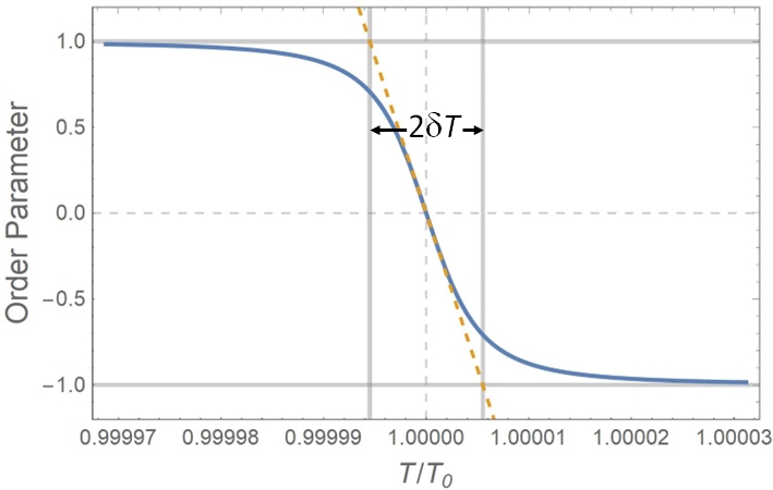
which satisfies the following two conditions: (i) and cross at , and (ii) except for an ultra-narrow temperature region around . The width of the crossover can be estimated by solving at . This definition of is consistent with the crossover width later defined by measuring the order parameter [see Eq. (37)]. Eq. (3) looks the same as Eq. (2) except when zoomed into the ultra-narrow region around (see Fig. 1b).
The form of Eq. (3) can result from the 1D Ising model on a single chain. In the thermodynamic limit, the free energy per unit cell , where is the number of unit cells, is the partition function, and with being the Boltzmann constant. of a 1D Ising model can be obtained exactly by using the transfer matrix method Mattis_book_08_SMMS ; Mattis_book_1985 ; Baxter_book_Ising ; 003_Huang_08_book ; Mejdani_Ising_ladder ; 005_Galisova_PRE_15_double-tetrahedral-chain ; 007_Torrico_PRA_16_Ising-XYZ-diamond-chain ; 009_review_Souza_SSC_18_Ising-XYZ-diamond-chain_double-tetrahedral-chain-spin-electron ; 010_Carvalho_JMMM_18_Ising-XYZ-diamond-chain_quantum-entanglement ; 011_Rojas_BJP_20_Ising-Heisenberg-tetrahedral_diamond ; 013_Rojas_PRE_19_previous_4_models ; 014_Rojas_JPC_20_Ising–Heisenberg_spin-1-double-tetrahedral-chain ; 015_Strecka_APPA_20_Ising-diamond-chain ; 015-7_Canova_CzechoslovakJP_04_Ising–Heisenberg_diamond_chain ; 015-8_Canova_JPC_06_Ising–Heisenberg-spin-S-diamond-chain ; 017_Krokhmalskii_PA_21_3-previous-chains_effective_model ; 016_Strecka_book_chapter ; 008_zero-field_Rojas_SSC_16_Ising-Heisenberg_ladder ; 006_zero-field_Strecka_JMMM_16_Ising-Heisenberg-3-leg-tube ; Yin_MPT ; Yin_icecreamcone and is given by
| (4) |
where is the transfer matrix, the th eigenvalue of , and the largest eigenvalue. Thus, . For the single-chain Ising model, the transfer matrix is of the following form:
| (7) |
with . Compared with Eq. (3), is of the same form when the function is defined as .
II.2 The absence of SMPT in single-chain Ising models
However, in the absence of the bias (), the Ising model is invariant with respect to flipping all . By this spin up-down symmetry, and in Eq. (7) for single-chain Ising models, including decorated Ising chains. This means the absence of SMPT, which requires the crossing of and as changes.
The nonzero bias breaks the above invariance and lifts the degeneracy of and . For the simplest single-chain model, , , . Thus, and do not cross at all. How to make and cross in decorated single-chain Ising models in the presence of the bias was the subject of the so-called “pseudo transition” 005_Galisova_PRE_15_double-tetrahedral-chain ; 007_Torrico_PRA_16_Ising-XYZ-diamond-chain ; 009_review_Souza_SSC_18_Ising-XYZ-diamond-chain_double-tetrahedral-chain-spin-electron ; 010_Carvalho_JMMM_18_Ising-XYZ-diamond-chain_quantum-entanglement ; 011_Rojas_BJP_20_Ising-Heisenberg-tetrahedral_diamond ; 013_Rojas_PRE_19_previous_4_models ; 014_Rojas_JPC_20_Ising–Heisenberg_spin-1-double-tetrahedral-chain ; 015_Strecka_APPA_20_Ising-diamond-chain ; 015-7_Canova_CzechoslovakJP_04_Ising–Heisenberg_diamond_chain ; 015-8_Canova_JPC_06_Ising–Heisenberg-spin-S-diamond-chain ; 017_Krokhmalskii_PA_21_3-previous-chains_effective_model ; 016_Strecka_book_chapter . It was understood that certain decorations could renormalize the bias to be effectively -dependent and the resulting changes its sign at the pseudo-critical temperature 017_Krokhmalskii_PA_21_3-previous-chains_effective_model . Nevertheless, vanishes for , in agreement with the aforementioned spin up-down symmetry. Therefore, no spontaneous pseudo-transition would occur in those systems.
The extensively studied 1D Ising chain with the first- and second-nearest-neighbor interactions, the - model Fleszar_Baskaran_JPC_85_J1-J2 ; Stephenson_CanJP_70_J1-J2-Ising-chain ; Dobson_JMathP_69_Many‐Neighbored-Ising-Chain ; Dhar_PRE_00_J1-J2-Ising-chain , showcases the emerging of an effective magnetic field for by the transformation . This was inspiring. However, , the nearest-neighbor interaction, is not -dependent, and the transformed model is an ordinary single-chain Ising model in this -independent effective field Fleszar_Baskaran_JPC_85_J1-J2 ; Stephenson_CanJP_70_J1-J2-Ising-chain ; Dobson_JMathP_69_Many‐Neighbored-Ising-Chain . Therefore, the resultant effective and do not cross at all.
II.3 Dimensionality increase and reduction for SMPT
To find SMPT, we resort to the strategy of dimensionality increase and reduction: First, we increase the transfer matrix from to . Then, we identify the transfer matrix that has such high symmetry that it can be block diagonalized and reduced back to a matrix Mattis_book_08_SMMS now with the new effective and crossing.
We consider the following transfer matrix
| (12) |
It can be block diagonalized by the parity-symmetry operations :
| (17) |
and the result is
| (22) |
Thus, the eigenvalues of the transfer matrix are , , and
| (23) |
Then, the task is transformed to how to realize the crossing of and .
The transfer matrix can be obtained for the 1D Ising model on a 2-leg ladder. The ordinary 2-leg Ising ladder Mejdani_Ising_ladder , the spin-1/2 Ising tetrahedral chain 016_Strecka_book_chapter , and the spin-1/2 Ising-Heisenberg ladder with alternating Ising and Heisenberg inter–leg couplings 008_zero-field_Rojas_SSC_16_Ising-Heisenberg_ladder are known special cases satisfying the symmetry of Eq. (12). Among them, the ordinary 2-leg ladder does not host the SMPT, and the latter two cases with zero-field pseudo-transition have not been analyzed with the above symmetry-based block diagonalization technique, which is vital to systematically looking for more cases of spontaneous ultra-narrow phases crossover. Here, we take the ordinary 2-leg ladder as the parent system and investigate how to properly decorate it with child spins.
III A minimal model
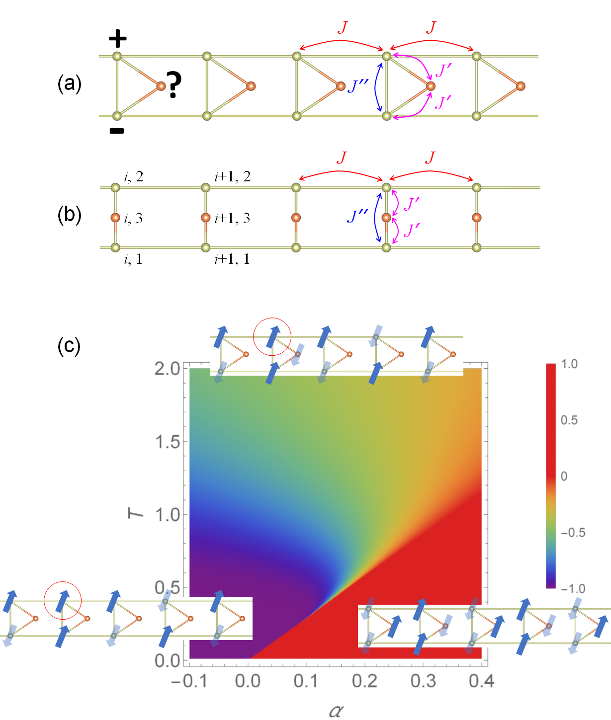
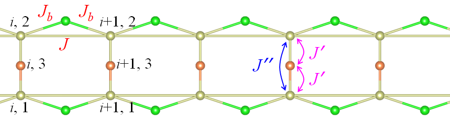
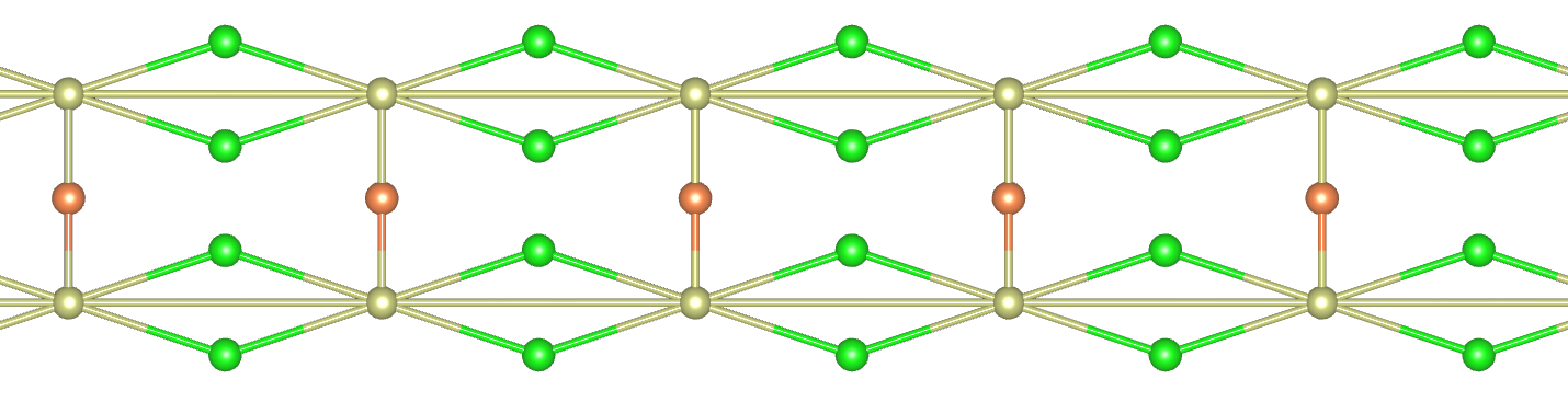
For clarity, we focus the presentation on the trimer-rung ladder that has only one decorated spin per rung in this section. The spin trimer (Fig. 2b) or equivalently triangular (Fig. 2a; hence the source of frustration is more obvious) represents the simplest form of frustration. The model is defined as
| (24) | |||||
where denotes the spins on the th site of the th rung of the ladder and (i.e., the periodic boundary condition). is the total number of the rungs and we are interested in the thermodynamical limit . Each rung has three sites with on the two legs (referred to as the parent sites) and decorated at the middle (referred to as the child site) of the rung; so a rung is also called a household for ease of memory. is the nearest-neighbor interaction along the legs, the interaction that directly couples the two legs, and the interaction that couples the child spin to the two parent spins ( reduces the system to the ordinary 2-leg ladder); and are intra-household. The parameter space for strong frustration can be estimated from the limit, in which the system is reduced to decoupled trimers or triangles: (antiferromagnetic interaction) and . In the following, the frustration is parameterized by
| (25) |
The smaller the magnitude of , the stronger the frustration. To make the ground state have much less degeneracy or entropy, the two parent spins of a household must have the same value by coupling more strongly to the child spin via than their direct antiferromagnetic coupling , i.e., .
III.1 The transfer matrix and SMPT
Since the model has three spins and possible states per unit cell, its transfer matrix is at a glance. However, the child spins can be exactly summed out as they are coupled only to the parent spins on the same rung, yielding the children’s contribution functions
| (26) |
They are translationally invariant, i.e., . Then, using the spin up-down symmetry, i.e., and , we found the transfer matrix in the order of to be of the same form as Eq. (12), with , , , , and .
The largest eigenvalue of the transfer matrix is
| (27) |
with the household’s frustration functions
| (28) | |||||
which are controlled by the intra-household interactions and , but independent of the inter-houseld interaction . Here we have used the relationship and . depends on and solely via . Note that the equations of (27) and (28) are invariant upon the transformation of or (i.e., ferromagnetic and antiferromagnetic interactions are interchangeable), but they are not for . That is, only (antiferromagnetic interaction) introduces frustration.
measures the crossing of and . It changes sign at where , i.e.,
| (29) |
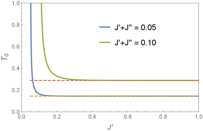
This means that is determined only by the on-rung interactions , and independent of the on-leg interaction . For sufficiently large , ,
| (30) | |||||
For example, for and yielding . As shown in Fig. 3(a), for to keep , as a function of estimated by Eq. (30) (dashed lines) accurately reproduces the exact results of Eq. (29) (solid lines) except for where increases exponentially; indeed, in the unfrustrated limit of , and no crossover would happen at finite temperature.
It is now clear that SMPT was not found in the ordinary 2-leg ladder without the children. In that case, leads to , which does not change sign for given . For as the other limit of no frustration, does not change sign, either.
Secondly, in Eq. (27) has a prefactor of , which scales as in the vicinity of . So, if Eq. (27) is approximated by neglecting 1 inside for the strong frustration of ,
| (31) |
which becomes non-analytic. The difference between Eq. (27) and Eq. (31) takes place in a region of , where the crossover width can be estimated by at , yielding
| (32) | |||||
| (33) |
where Eq. (32) is exact and Eq. (33) is based on Eq. (30). has two paths to approach zero: (i) , which is not unexpected as zero-temperature phase transition is allowed. (ii) For fixed finite , which is determined by and , the width approaches zero exponentially as increases. Using the above example of , and for and , respectively. Note that for both cases by Eqs. (25) and (30). Although the proof of nonexistence of any phase transition in 1D Ising models with short-range interactions based on the Perron–Frobenius theorem does not work for infinite-strength interactions Cuesta_1D_PT , similar to zero temperature, it is amazing to realize such an ideal paradigm of SMPT in which and are controlled by different model parameters and for fixed , decays exponentially with the single parameter . This issue will be further addressed in Section IV.
III.2 Thermodynamic properties
The thermodynamical properties can be retrieved from the free energy per trimer , the entropy , and the specific heat .
We compare the free energies per trimer obtained from using the exact Eq. (27) (Fig. 1b) and the mimicked Eq. (31) (Fig. 1a) for ; they differ within sub-millikelvins for K when the slope changes from near 0 to near . The SMPT resembles a first-order phase transition with the large latent heat of per trimer.
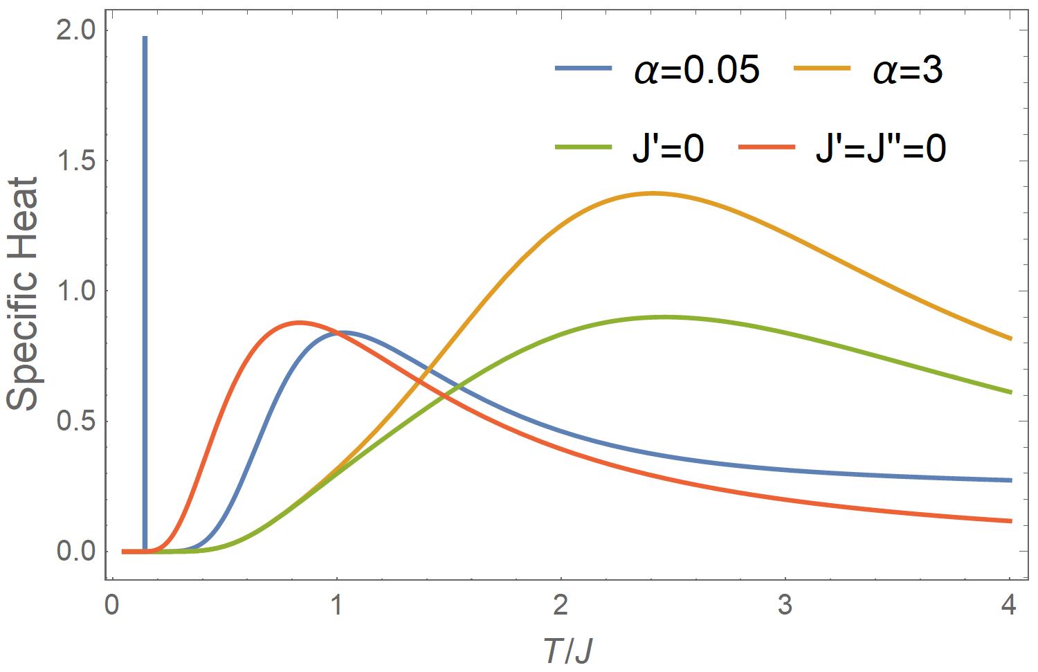
Fig. 3b shows a sharp peak in the exact specific heat for (blue line), resembling a second-order phase transition. In comparison, the three typical unfrustrated cases, namely (i) or governed by (orange line), (ii) the ordinary 2-leg ladder governed by (green line), and (iii) the decoupled double chains (red line), do not show such a sharp peak.
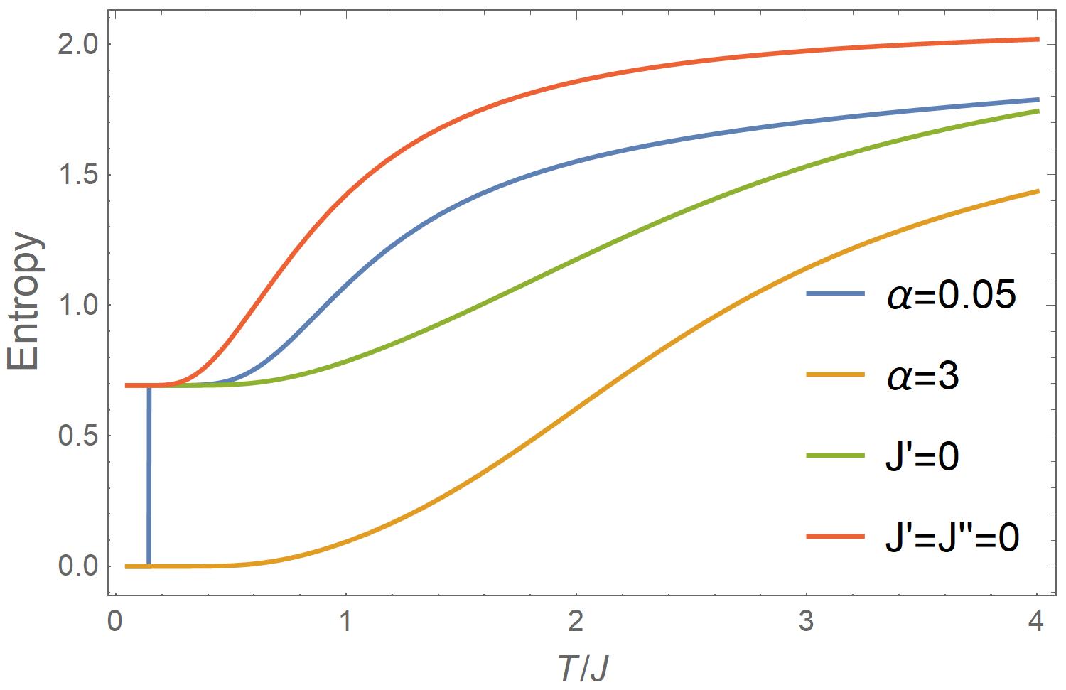
Fig. 3c show the temperature dependence of the exact entropy for the same four cases as Fig. 3b. The strongly frustrated case for (blue line) shows a waterfall behavior at , where the entropy falls vertically (within ) from a plateau at down to zero. Its low- zero-entropy behavior is in line with the unfrustrated case for (orange line), while its intermediate- -plateau behavior is in line with the ordinary 2-leg ladder case for (green line) where the child spins are completely decoupled from the system and thus yield the specific entropy of . This offers a hint to the nature of the SMPT: it is an entropy-driven transition, in which the child spins are tightly coupled to the two parent spins on the legs in the low- region because , but they are decoupled from the outer ones in the intermediate- region just above thanks to the jumping contribution of entropy in terms of to the free energy. Mathematically, in the temperature region near , one can estimate from Eq. (31) that below and above , i.e., the low- region is controlled by , while the intermediate- region is controlled by with the decoupled child spin contributing the factor of 2 to and to entropy. Moreover, in the high- region beyond the plateau, the entropy does not continue following the ordinary 2-leg ladder case (green line) but behaves closer to the decoupled double chains for (red line). A similar behavior also shows up in the high- region of the specific heat (Fig. 3a), indicating that frustration effectively decouples the chains. We shall come back to understand this strange behavior soon.
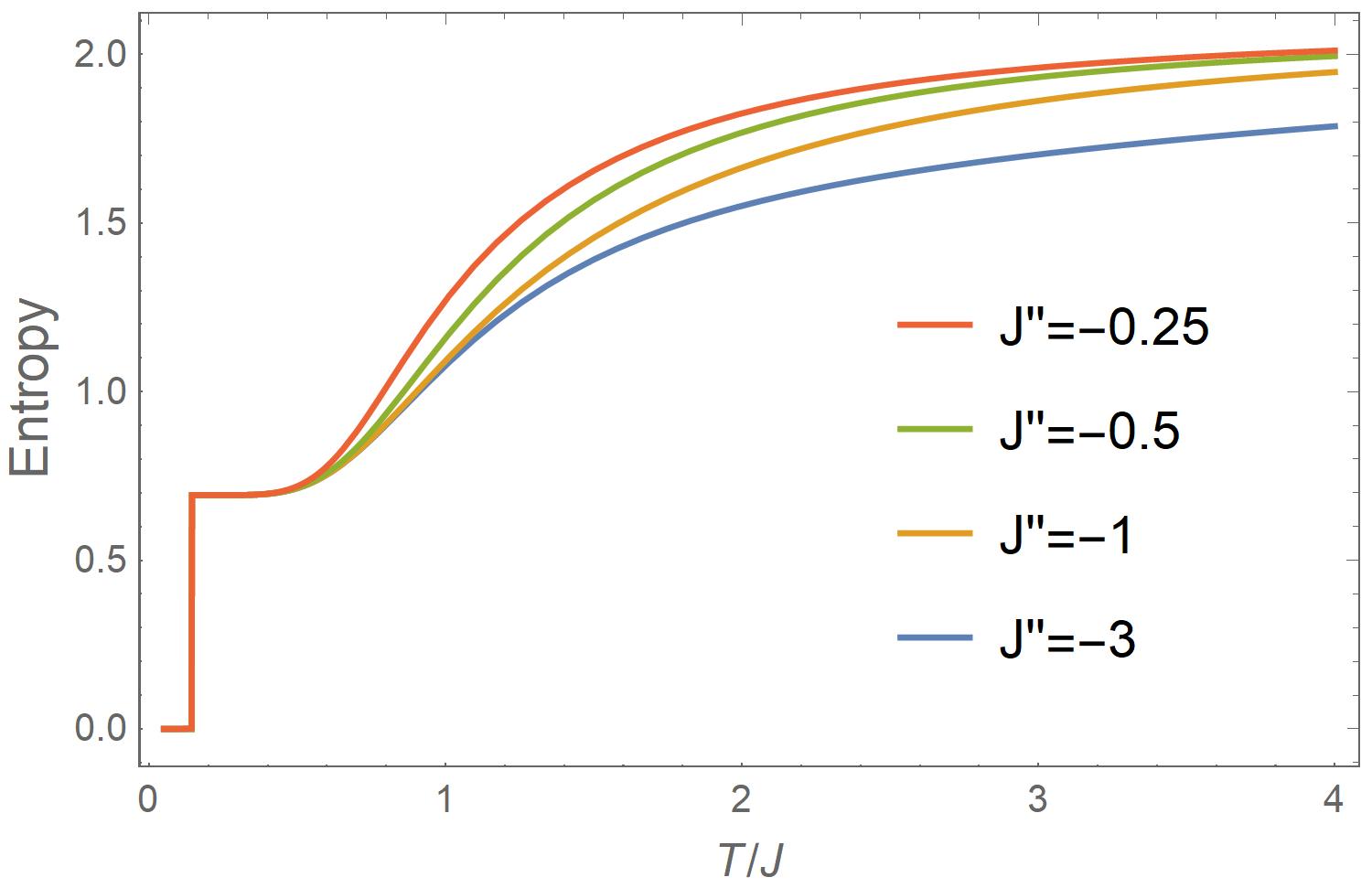
For the revealed three -region behavior of the specific entropy, Eqs. (30) and (32) determine that the SMPT itself is a sole function of . This is demonstrated in Fig. 3d for fixed but with different , which directly couples the two legs: The lines overlap in the first two -regions surrounding the waterfall at . In contrast, in the high- region, the detail behavior of spin frustration is sensitive to (and shown below). It is understandable that as and decreases, the entropy moves up to be closer to the case of the decoupled double chains. What is strange is why the chains with strong inter-chain interactions also appear to be decoupled.
III.3 Spin-spin correlation functions and order parameters
To find an appropriate order parameter that describes the three regions and the associated transitions, we proceed to calculate the spin-spin correlation functions, which allow us to have detailed site-by-site information:
| (34) |
where denotes the thermodynamical average, is the eigenvector of the transfer matrix corresponding to the largest eigenvalue and is the eigenvector corresponding to the th eigenvalue . So, .
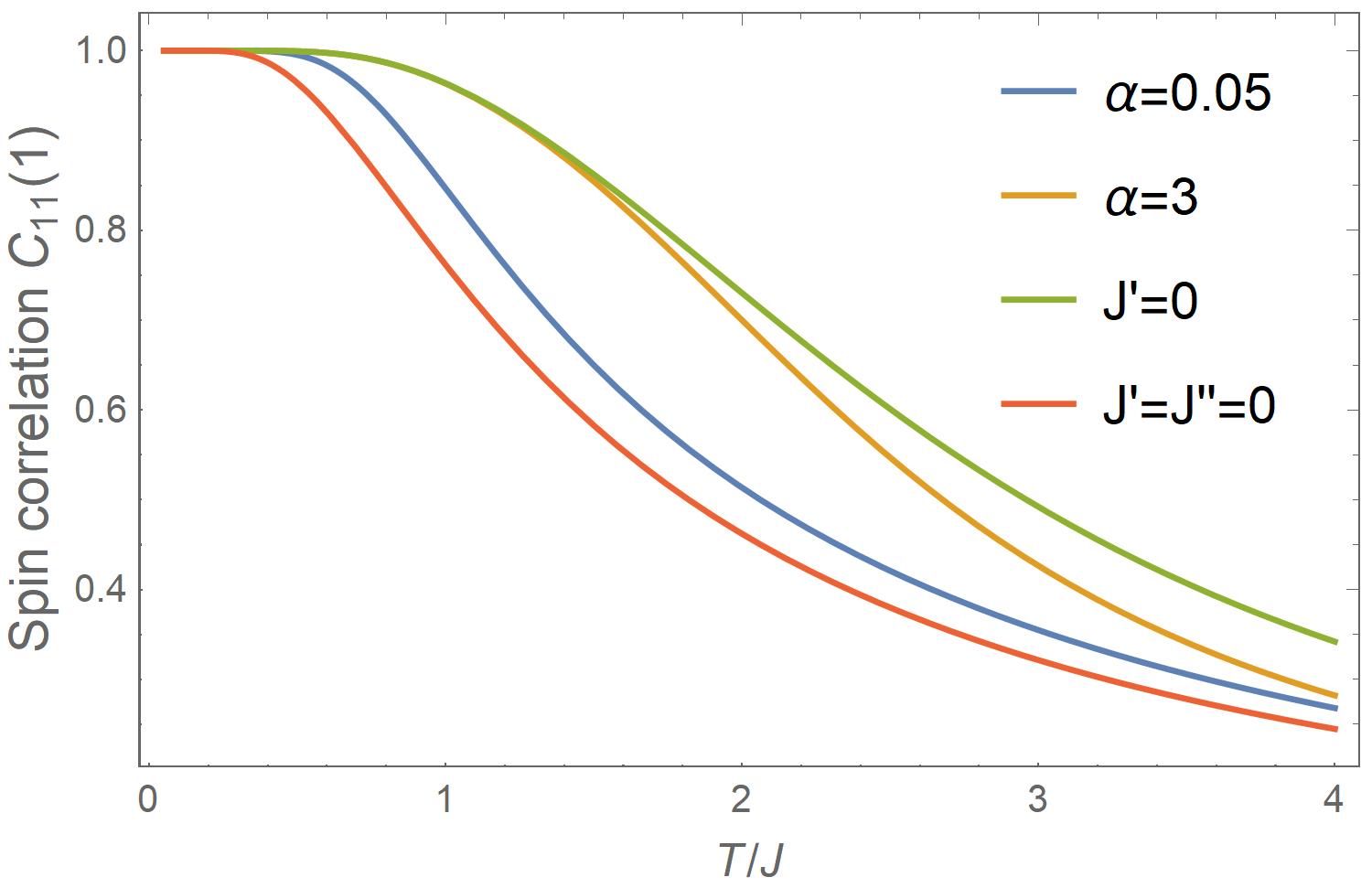
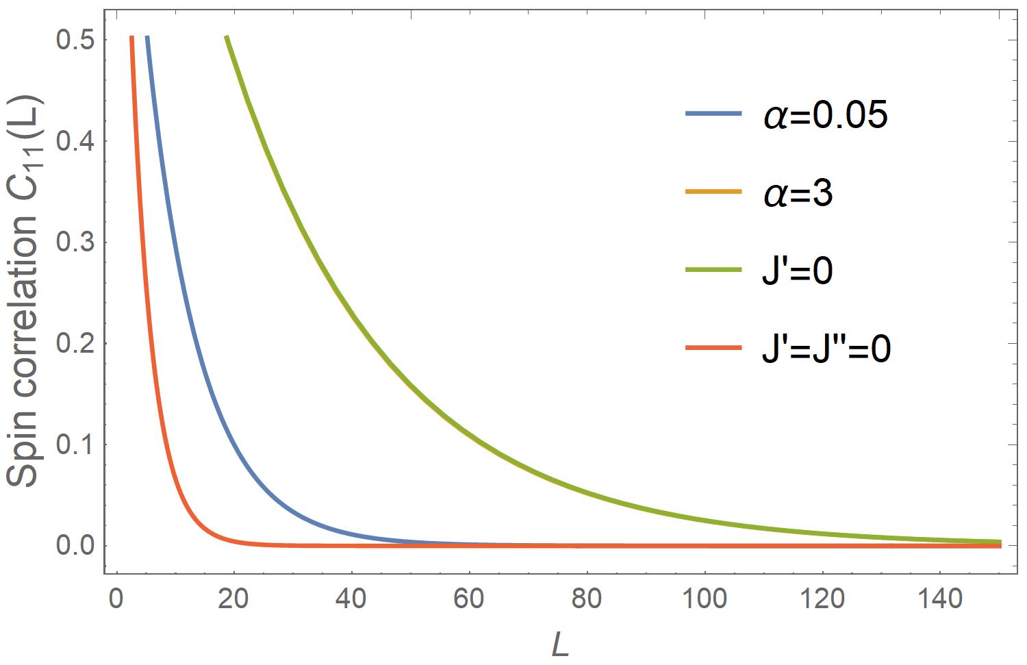
As shown in Figs. 4c and 4d, the behavior of intra-chain correlation as a function of both and (blue lines) is closer to the decoupled double chains of (red lines), consistent with the specific heat (Fig. 3b) and the entropy data (Fig. 3c). The data of the unfrustrated yet strongly coupled chains for both (orange lines) and (green lines) cases move to considerably higher temperatures, suggesting that the chain decoupling is related to the energy cost for attempts to break the order.
The conventional choice of the order parameter is the magnetization at finite . This agrees with the theorems about the nonexistence of finite- phase transition in 1D Ising models with short-range interactions Cuesta_1D_PT . Hence, the magnetization cannot be used as the order parameter for the SMPT. Instead, let us look at the on-rung correlation function :
| (35) | |||||
| (36) |
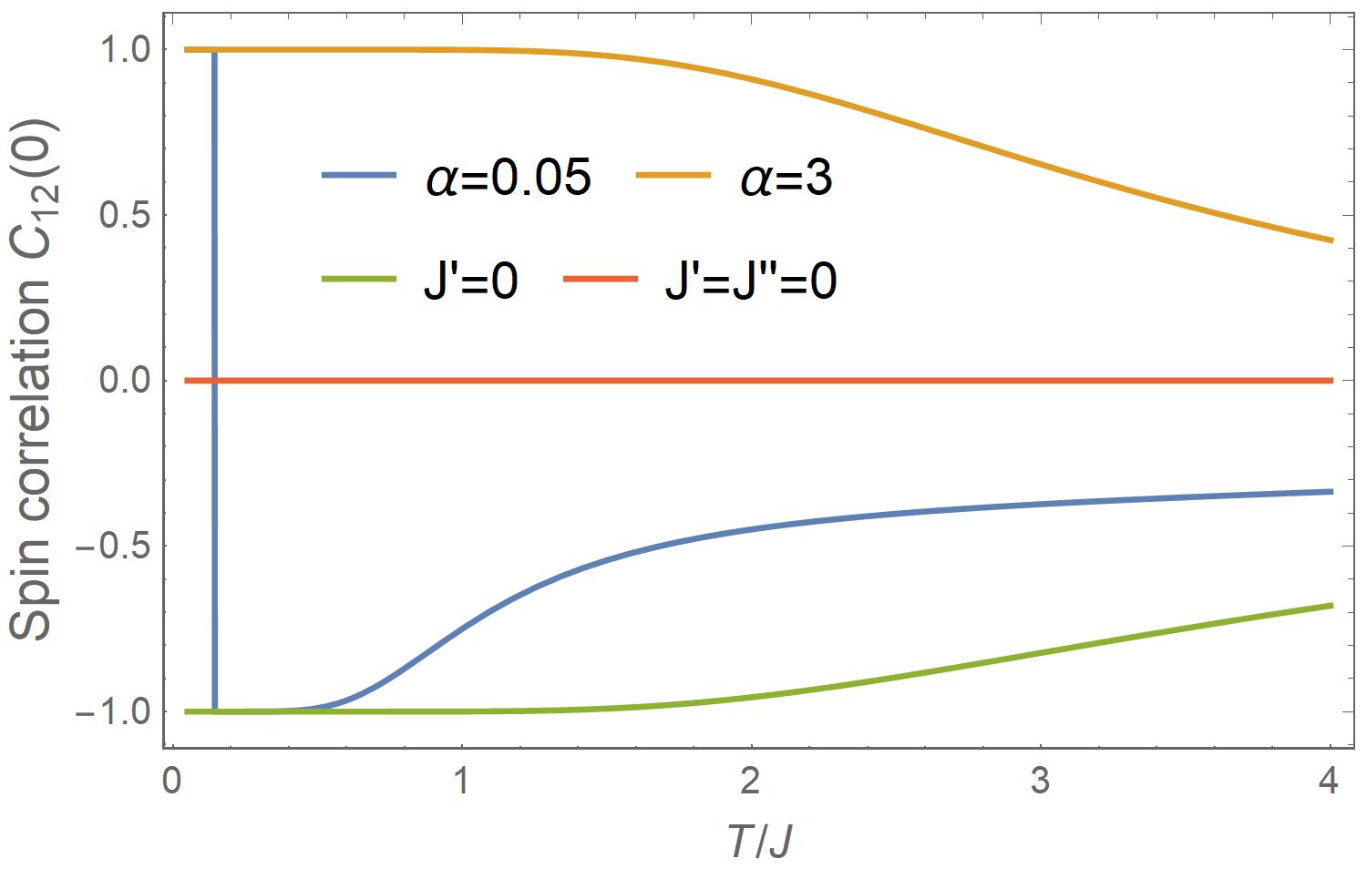
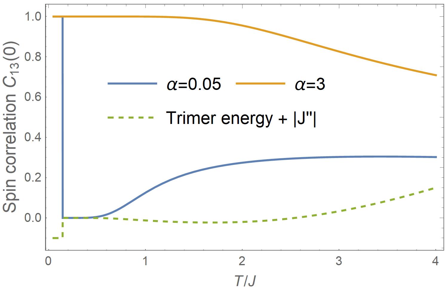
, the correlation between two parent spins on the legs, is proportional to the frustration function and changes sign at (exactly zero at ). Because of the exponentially large and near , below and above , as shown in Fig. 4a (blue line for ). Below , the blue line overlaps with the unfrustrated -dominated case of (orange line). In the intermediate- region, it shows a plateau and overlaps with the unfrustrated -dominated ordinary 2-leg ladder case (green line). That is, the two parent spins changes from having like values in the low- region to having unlike values in the intermediate- region where the child spins appear to be decoupled from the ladder. So, one rung’s contribution to the free energy for and is approximately and , respectively. They cross at , in agreement with Eq. (30). What is remarkably new to learn is that for the high- region, while remaining negative, the blue line of does not continue following the green line, which gradually decays to zero as temperature increases. Instead, it decays significantly faster with an inflection point at before gradually decaying to zero. Yet, with at , it is still far away from the zero red line for the case of the completely decoupled double chains. The two chains seem to be strongly coupled. How can we reconcile this with the effective decoupling seen in the above thermodynamic properties and the intra-chain correlation functions?
The answer is Eq. (36) for and , the correlations between the child spin and the two parent spins on the same rung. They are equal by symmetry. Since just told us that spin 1 and spin 2 on the same rung strongly want to have unlike values, it would have been expected in static mean-field theory that and should have opposite signs; considering that they are required to be equal by symmetry, they should be zero. Indeed, in the intermediate- region, is nearly zero (blue line in Fig. 4b). However, as soon as the temperature increases beyond the intermediate- region, jumps up, meanwhile the magnitude of decreases (blue line in Fig. 4a). This means that the child spin starts to re-couple to the parent spins to gain energy at the expense of , following the astonishing near-linear relationship of Eq. (36). The total energy within one trimer remains nearly unchanged in a wide range of temperatures (dashed line in Fig. 4b), which indicates that the trimers can self-organize to relieve energy cost in their value-changing dynamics. Sizable encourages the two parent spins to have like values, which counters negative . The net effect is decoupling the two legs.
The correlation length of the two-spin quantities is infinite at , since the four-spin correlation function is not vanishing. Therefore, are bona fide order parameters. To check with the ordinary ladders, Figs. 4a and 4b show that and can be finite for the other three unfrustrated cases; however, they do not change sign or they are vanishing only at . This means that using as the order parameters for the ordinary unfrustrated cases still satisfies the theorems that no phase transitions take place at finite temperature in those systems. Therefore, the unconventional order parameters can unify the description of both the ordinary 2-leg ladder system and the unconventional phase transitions in the present frustrated ladder Ising model.
To further verify that is a bona fide order parameter, we redefine the crossover width by measuring the slope of at as shown in Fig. 6(a):
| (37) | |||||
| (38) |
which differs from the previous definition of in Eq. (32) by replacing with . They are consistent as for an ultra-narrow phase crossover. Therefore, this nonclassical order parameter, which has a well-defined value space of with the value meaning and its inverse slope at meaning , provides an accurate, convenient, and microscopic description of SMPT.
The phase diagram in terms of the unconventional order parameter is shown in Fig. 2c. The frustrated 2-leg ladder Ising model can have three phases for : (i) the low- phase (red zone) is governed by forcing the two parent spins on the same rung to have like values. (ii) The intermediate- phase (purple zone) is governed by forcing the two parent spins on the same rung to have unlike values and the child spin to be decoupled. The abrupt switching between the two phases is an entropy-driven SMPT with large latent heat, resembling the first-order phase transition. (iii) The exotic high- phase (blue-green zone) is governed by the dynamics of the frustration. The much broader crossover between the intermediate- phase and the exotic high- phase reveals itself via the phenomenon of frustration-driven decoupling of the strongly interacted chains. The microscopic mechanism for the decoupling is illustrated in Fig. 2c, where the high energy cost associated with the thermal activated flipping of a parent spin in the strongly interacted double chains can be relieved in the trimer dynamics by flipping the child spin cooperatively. The exact result of sizeable nonzero demonstrates that the child spin is not a slave to the mean field generated by the two parent spins, but they have equal rights. The dynamics of the trimers exhibits the art of compromise and finds the way to have created a triple-win workplace in which every neighboring bond gains an optimized share of rewards.
IV The asymptoticity
We proceed to discuss how to arbitrarily approach the genuine phase transition at finite temperature, i.e., for fixed . This hard task becomes obvious in our model, since the value of is determined by and , while the width approaches zero exponentially as increases for fixed . Nevertheless, we hereby ask how we can improve the asymptoticity if has to be fixed or its strength cannot be further increased.
One simple answer is to effectively enhance by decorating the legs in such a symmetric way that the resulting transfer matrix—after the decorated spins (referred to as the bridge sites) are summed out—is of the same form as Eq. (12). The convenience of using effective interactions was emphasized recently in the context of pseudo-transition 017_Krokhmalskii_PA_21_3-previous-chains_effective_model and extended to study Eq. (24) the minimal model for SMPT Hutak_PLA_21_trimer soon after the model appeared in arXiv Yin_MPT ; Yin_icecreamcone . We will show that the decoration of the legs (which controls ) can be done independently of the decoration of the rungs (which controls ), revealing an amazing advantage of this paradigm.
For simplicity, we consider identical bridge sites for each bond on the legs; the bridge sites do not interact with one another (Fig. 5). Thus, we add the term to the model Hamiltonian Eq. (24):
| (39) |
where is the Ising spin on the th of the bridges connecting the th and th parent spins on the th leg.
Like the child spins, the bridge spins can be exactly summed out, yielding the bridges’ contribution functions
| (40) |
They are translationally invariant and identical for both legs, i.e., . Then, using the spin up-down symmetry, i.e., and , we found the transfer matrix in the order of to be of the same form as Eq. (12), with , , , , and .
We found that after introducing the following effective in the place of ,
| (41) | |||||
| (42) |
which is independent of the on-rung (intra-household) interactions, the partition function remains the same except for an additional factor of . This means that the household’s frustration functions are the same as defined in Eq. (28) and after substituting for , the order parameter looks the same, too:
| (43) |
Note that for . At the relevant low temperature,
| (44) |
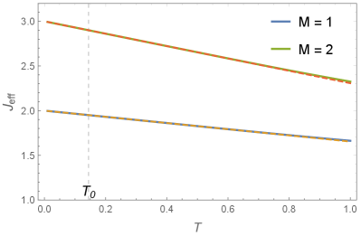
that is, the effect of this bridge decoration is to enhance by about for ferromagnetic . As shown in Fig. 6c, as a function of estimated by Eq. (44) (dashed lines) accurately reproduces the exact results of Eq. (42) (solid lines).
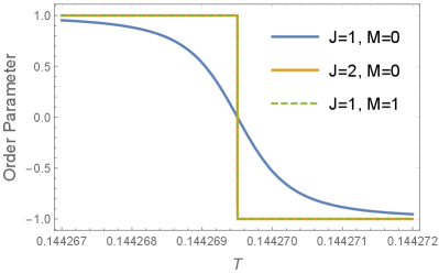
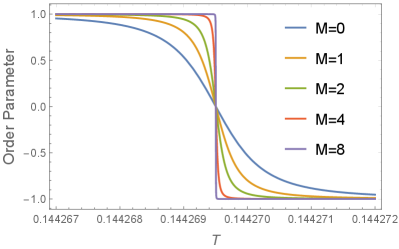
The order parameter shows in Fig. 6b that with doubled (red solid line) and the decoration of with (green dashed line) have almost the same effect on the exponential reduction of the crossover width from to , given , in agreement with Eq. (44). Therefore, we can improve the asymptoticity by adding those bridges if has to be fixed or its strength cannot be further increased. To see the effect of more clearly, we present in Fig. 6d the results with . The SMPT becomes exponentially narrower and narrower as increases, manifesting the asymptoticity of the SMPT and making it clear that spontaneous phase transition at finite temperature does not exist in the 1D Ising model with a finite number of short-range interactions.
The present model can be be easily extended to the case of multiple coupled children and coupled bridges. In Eq. (26) and Eq. (40) for the children’s and bridges’ contribution functions, respectively, the detailed form of or is unlimited. It works for arbitrary forms of interactions among the children in the same household (among the bridges between the same pair of the parents) and for both classical and quantum children/bridges—as long as their interactions with the parents are of Ising type—because the commutator and . So, the children/bridges can be more than spins. They can be electrons, phonons, excitons, Cooper pairs, fractons, anyons, etc. For the systems with mixed quantum particles and classical Ising spins 006_zero-field_Strecka_JMMM_16_Ising-Heisenberg-3-leg-tube ; 008_zero-field_Rojas_SSC_16_Ising-Heisenberg_ladder ; 011_Rojas_BJP_20_Ising-Heisenberg-tetrahedral_diamond ; 014_Rojas_JPC_20_Ising–Heisenberg_spin-1-double-tetrahedral-chain ; 015-7_Canova_CzechoslovakJP_04_Ising–Heisenberg_diamond_chain ; 015-8_Canova_JPC_06_Ising–Heisenberg-spin-S-diamond-chain , one first obtains the eigenvalues (energy levels) of the quantum Hamiltonian for one of the four combinations of the spin configurations of the parents in the same household, say , and thermally populates those energy levels to get . Then move on to work out for the other three combinations one by one. Likewise, for quantum , work out the four combinations of the spin configurations of the nearest-neighbor parents on the same leg. Such diversity generates an infinite number of 1D systems with SMPT. The urgent questions as to how to classify nontrivial cases and reveal more and more novel effects of SMPT will be addressed in subsequent publications Yin_icecreamcone .
V Open questions
Given the prominent roles of the Ising model and frustration in understanding collective phenomena in various physical, biological, economical, and social systems, and the prominent roles of 1D systems in research, education, and technology applications, we anticipate that the present new insights to phase transitions and the dynamical actions of frustration will stimulate further research and development about MPT. We thus leave a few open questions as our closing remarks:
(1) What are other asymptotic paths of SMPT for ? Moreover, given the present success in finding SMPT, we reconsider : what is a simple paradigm for in-field asymptotic MPT at a fixed finite temperature ? In general, the presence of the magnetic field will break the high symmetry of the matrix shown in Eq. (12), making it irreducible to the matrix needed for the present analysis. These challenges are expected to serve as a driving force for further exploration of possibilities in functionalities and their optimized performance within the huge capacity of the infinite number of 1D systems with MPT in the absence or presence of a bias (magnetic) field.
(2) What are the first-generation SMPT-ready 1D devices for thermal applications? This appears to be feasible right now, since the Ising model has already been implemented in electronic circuits Ising_FPGA and optical networks Pierangeli_IsingMachine_PRL19 . The features that and can be independently controlled by different parameters and different decoration methods could be attractive in engineering 1D thermal sensors, for example.
(3) In the SMPT, the intermediate-temperature phase (ITP) is not a conventional, fluctuating or short-range ordered continuation of the low-temperature phase (LTP). The essence of strong frustration in driving SMPT is that the ITP is slightly higher in energy than the LTP but possesses gigantic entropy Miyashita_10_review_frustration as some degrees of freedom in the ITP decouple from the rest of the system. The appearance of such an ITP is reminiscent of recently discovered strange fluctuating orbital-degeneracy-lifted states at intermediate temperature in CuIr2S4 and other materials with active orbital degrees of freedom Bozin_NC_CuIr2S4 . To date, the commonly known effect of strong frustration is to dramatically suppress (the critical temperature at the spontaneous phase transition) despite strong interactions, as seen in many frustrated magnets Balents_nature_frustration ; hence, frustration has been regarded as a driver for achieving spin liquids, which do not order down to zero temperature Balents_nature_frustration ; Cao_npjQM_Ba4Ir3O10 ; Yin_PRL_22_trimer ; Yin_PRB_21_trimer . Could the present exact lesson encourage the use of strong frustration to understand, control, and engineer more and more LTP-ITP transitions in real materials?
(4) In a broader sense, the idea of pushing the limit in our knowledge as close as possible to the forbidden regime can be applied to other domains. For example, the Mermin–Wagner theorem Mermin_PRL_theorem rules out spontaneous phase transition at finite temperature in 1D or 2D isotropic Heisenberg models for quantum spins with short-range interactions. Now we ask: Does a SMPT at finite temperature exist in those quantum systems?
Acknowledgements.
The author is grateful to D. C. Mattis for mailing him a copy of Ref. Mattis_book_08_SMMS as a gift and inspiring discussions over the years. Brookhaven National Laboratory was supported by U.S. Department of Energy (DOE) Office of Basic Energy Sciences (BES) Division of Materials Sciences and Engineering under contract No. DE-SC0012704.References
- (1) Mattis, D. C. & Swendsen, R. Statistical Mechanics Made Simple (WORLD SCIENTIFIC, 2008), 2nd edn. URL https://www.worldscientific.com/doi/abs/10.1142/6670. eprint https://www.worldscientific.com/doi/pdf/10.1142/6670.
- (2) Mattis, D. C. The Theory of Magnetism II (Springer, Berlin, Heidelberg, 1985). URL https://doi.org/10.1007/978-3-642-82405-0.
- (3) Baxter, R. J. Exactly Solved Models in Statistical Mechanics (Academic Press, 1982).
- (4) Huang, K. Statistical mechanics (John Wiley & Sons, 2008).
- (5) Ising, E. Beitrag zur theorie des ferromagnetismus. Zeitschrift für Physik 31, 253–258 (1925). URL https://doi.org/10.1007/BF02980577.
- (6) Onsager, L. Crystal statistics. i. a two-dimensional model with an order-disorder transition. Phys. Rev. 65, 117–149 (1944). URL https://link.aps.org/doi/10.1103/PhysRev.65.117.
- (7) Dagotto, E. & Rice, T. M. Surprises on the way from one- to two-dimensional quantum magnets: The ladder materials. Science 271, 618–623 (1996). URL https://science.sciencemag.org/content/271/5249/618. eprint https://science.sciencemag.org/content/271/5249/618.full.pdf.
- (8) Mejdani, R., Gashi, A., Ciftja, O. & Lambros, A. Ladder ising spin configurations ii. magnetic properties. physica status solidi (b) 197, 153–164 (1996). URL https://onlinelibrary.wiley.com/doi/abs/10.1002/pssb.2221970122. eprint https://onlinelibrary.wiley.com/doi/pdf/10.1002/pssb.2221970122.
- (9) Cuesta, J. A. & Sánchez, A. General non-existence theorem for phase transitions in one-dimensional systems with short range interactions, and physical examples of such transitions. Journal of Statistical Physics 115, 869–893 (2004). URL https://doi.org/10.1023/B:JOSS.0000022373.63640.4e.
- (10) Batista, C. D. & Nussinov, Z. Generalized elitzur’s theorem and dimensional reductions. Phys. Rev. B 72, 045137 (2005). URL https://link.aps.org/doi/10.1103/PhysRevB.72.045137.
- (11) Gálisová, L. & Strečka, J. Vigorous thermal excitations in a double-tetrahedral chain of localized ising spins and mobile electrons mimic a temperature-driven first-order phase transition. Phys. Rev. E 91, 022134 (2015). URL https://link.aps.org/doi/10.1103/PhysRevE.91.022134.
- (12) Torrico, J., Rojas, M., de Souza, S. & Rojas, O. Zero temperature non-plateau magnetization and magnetocaloric effect in an ising-xyz diamond chain structure. Physics Letters A 380, 3655–3660 (2016). URL https://www.sciencedirect.com/science/article/pii/S0375960116305308.
- (13) de Souza, S. & Rojas, O. Quasi-phases and pseudo-transitions in one-dimensional models with nearest neighbor interactions. Solid State Communications 269, 131–134 (2018). URL https://www.sciencedirect.com/science/article/pii/S0038109817303319.
- (14) Carvalho, I., Torrico, J., de Souza, S., Rojas, M. & Rojas, O. Quantum entanglement in the neighborhood of pseudo-transition for a spin-1/2 ising-xyz diamond chain. Journal of Magnetism and Magnetic Materials 465, 323–327 (2018). URL https://www.sciencedirect.com/science/article/pii/S0304885317335114.
- (15) Rojas, O. A conjecture on the relationship between critical residual entropy and finite temperature pseudo-transitions of one-dimensional models. Brazilian Journal of Physics 50, 675–686 (2020). URL https://doi.org/10.1007/s13538-020-00773-8.
- (16) Rojas, O., Strečka, J., Lyra, M. L. & de Souza, S. M. Universality and quasicritical exponents of one-dimensional models displaying a quasitransition at finite temperatures. Phys. Rev. E 99, 042117 (2019). URL https://link.aps.org/doi/10.1103/PhysRevE.99.042117.
- (17) Rojas, O., Strečka, J., Derzhko, O. & de Souza, S. M. Peculiarities in pseudo-transitions of a mixed spin-(1/2, 1) ising–heisenberg double-tetrahedral chain in an external magnetic field. Journal of Physics: Condensed Matter 32, 035804 (2019). URL https://dx.doi.org/10.1088/1361-648X/ab4acc.
- (18) Strečka, J. Peculiarities in pseudo-transitions of a mixed spin-(1/2, 1) ising–heisenberg double-tetrahedral chain in an external magnetic field. Acta Physica Polonica A 137, 610 (2020). URL https://doi.org/10.12693/APhysPolA.137.610.
- (19) Čanová, L., Strečka, J. & Jaščur, M. Exact results of the ising-heisenberg model on the diamond chain with spin-1/2. Czechoslovak Journal of Physics 54, 579–582 (2004). URL https://doi.org/10.1007/s10582-004-0148-6.
- (20) Čanová, L., Strečka, J. & Jaščur, M. Geometric frustration in the class of exactly solvable ising–heisenberg diamond chains. Journal of Physics: Condensed Matter 18, 4967 (2006). URL https://dx.doi.org/10.1088/0953-8984/18/20/020.
- (21) Krokhmalskii, T., Hutak, T., Rojas, O., de Souza, S. M. & Derzhko, O. Towards low-temperature peculiarities of thermodynamic quantities for decorated spin chains. Physica A: Statistical Mechanics and its Applications 573, 125986 (2021). URL https://www.sciencedirect.com/science/article/pii/S0378437121002582.
- (22) Strečka, J. Pseudo-critical behavior of spin-1/2 ising diamond and tetrahedral chains, 63–86 (Nova Science Publishers, New York, 2020). URL "https://arxiv.org/abs/2002.06942". Preprint on arXiv:2002.06942.
- (23) Balents, L. Spin liquids in frustrated magnets. Nature 464, 199–208 (2010). URL https://doi.org/10.1038/nature08917.
- (24) Miyashita, S. Phase transition in spin systems with various types of fluctuations. Proceedings of the Japan Academy. Series B, Physical and biological sciences 86, 643–666 (2010). URL https://www.ncbi.nlm.nih.gov/pmc/articles/PMC3066537/.
- (25) Rojas, O., Strečka, J. & de Souza, S. Thermal entanglement and sharp specific-heat peak in an exactly solved spin-1/2 ising-heisenberg ladder with alternating ising and heisenberg inter–leg couplings. Solid State Communications 246, 68–75 (2016). URL https://www.sciencedirect.com/science/article/pii/S0038109816301880.
- (26) Strečka, J., Alécio, R. C., Lyra, M. L. & Rojas, O. Spin frustration of a spin-1/2 ising–heisenberg three-leg tube as an indispensable ground for thermal entanglement. Journal of Magnetism and Magnetic Materials 409, 124–133 (2016). URL https://www.sciencedirect.com/science/article/pii/S0304885316301925.
- (27) Yin, W. Frustration-driven unconventional phase transitions at finite temperature in a one-dimensional ladder ising model. arXiv:2006.08921 (2020). URL https://arxiv.org/abs/2006.08921.
- (28) Yin, W. Finding and classifying an infinite number of cases of the practically perfect phase transitions with highly tunable novel properties in the ising model in one dimension. arXiv:2006.15087 (2020). URL https://arxiv.org/abs/2006.15087.
- (29) Fleszar, A., Glazer, J. & Baskaran, G. A complex short-range order phase diagram in a one-dimensional spin model. Journal of Physics C: Solid State Physics 18, 5347–5353 (1985). URL https://doi.org/10.1088%2F0022-3719%2F18%2F27%2F020.
- (30) Stephenson, J. Two one-dimensional ising models with disorder points. Canadian Journal of Physics 48, 1724–1734 (1970). URL https://doi.org/10.1139/p70-217. eprint https://doi.org/10.1139/p70-217.
- (31) Dobson, J. F. Many‐Neighbored Ising Chain. Journal of Mathematical Physics 10, 40–45 (2003). URL https://doi.org/10.1063/1.1664757. eprint https://pubs.aip.org/aip/jmp/article-pdf/10/1/40/11319549/40_1_online.pdf.
- (32) Dhar, A., Shastry, B. S. & Dasgupta, C. Equilibrium and dynamical properties of the axial next-nearest-neighbor ising chain at the multiphase point. Phys. Rev. E 62, 1592–1600 (2000). URL https://link.aps.org/doi/10.1103/PhysRevE.62.1592.
- (33) Hutak, T., Krokhmalskii, T., Rojas, O., Martins de Souza, S. & Derzhko, O. Low-temperature thermodynamics of the two-leg ladder ising model with trimer rungs: A mystery explained. Physics Letters A 387, 127020 (2021). URL https://www.sciencedirect.com/science/article/pii/S0375960120308872.
- (34) Ortega-Zamorano, F., Montemurro, M. A., Cannas, S. A., Jerez, J. M. & Franco, L. Fpga hardware acceleration of monte carlo simulations for the ising model. IEEE Transactions on Parallel and Distributed Systems 27, 2618–2627 (2016). URL https://arxiv.org/abs/1602.03016.
- (35) Pierangeli, D., Marcucci, G. & Conti, C. Large-scale photonic ising machine by spatial light modulation. Phys. Rev. Lett. 122, 213902 (2019). URL https://link.aps.org/doi/10.1103/PhysRevLett.122.213902.
- (36) Bozin, E. S. et al. Local orbital degeneracy lifting as a precursor to an orbital-selective peierls transition. Nature Communications 10, 3638 (2019). URL https://doi.org/10.1038/s41467-019-11372-w.
- (37) Cao, G. et al. Quantum liquid from strange frustration in the trimer magnet ba4ir3o10. npj Quantum Materials 5, 26 (2020). URL https://doi.org/10.1038/s41535-020-0232-6.
- (38) Shen, Y. et al. Emergence of spinons in layered trimer iridate . Phys. Rev. Lett. 129, 207201 (2022). URL https://link.aps.org/doi/10.1103/PhysRevLett.129.207201.
- (39) Weichselbaum, A., Yin, W. & Tsvelik, A. M. Dimerization and spin decoupling in a two-leg heisenberg ladder with frustrated trimer rungs. Phys. Rev. B 103, 125120 (2021). URL https://link.aps.org/doi/10.1103/PhysRevB.103.125120.
- (40) Mermin, N. D. & Wagner, H. Absence of ferromagnetism or antiferromagnetism in one- or two-dimensional isotropic heisenberg models. Phys. Rev. Lett. 17, 1133–1136 (1966). URL https://link.aps.org/doi/10.1103/PhysRevLett.17.1133.
Author Information The author declares no competing interests. Correspondence and requests for materials should be addressed to W.Y. ([email protected]).