A Nyström Method for Scattering by a Two-layered Medium with a Rough Boundary
Abstract
This paper considers the problems of scattering of time-harmonic acoustic waves by a two-layered medium with a non-locally perturbed boundary (called a rough boundary in this paper) in two dimensions, where a Dirichlet or impedance boundary condition is imposed on the boundary. The two-layered medium is composed of two unbounded media with different physical properties and the interface between the two media is considered to be a planar surface. We formulate the considered scattering problems as the boundary value problems and prove that each boundary value problem has a unique solution by utilizing the integral equation method associated with the two-layered Green function. Moreover, we develop the Nyström method for numerically solving the considered boundary value problems, based on the proposed integral equation formulations. We establish the convergence results of the Nyström method with the convergence rates depending on the smoothness of the rough boundary. It is worth noting that in establishing the well-posedness of the boundary value problems as well as the convergence results of the Nyström method, an essential role is played by the investigation of the asymptotic properties of the two-layered Green function for small and large arguments. Finally, numerical experiments are carried out to show the effectiveness of the Nyström method.
Keywords: two-layered Green function, two-layered medium, integral equation method, Nyström method
1 Introduction
This paper is concerned with the well-posedness and the numerical method for the problems of scattering of time-harmonic acoustic waves in a two-layered medium in two dimensions. The two-layered medium is composed of two unbounded media with different physical properties and the interface between the two media is considered to be a planar surface. The boundary of the two-layered medium is assumed to be a rough surface, which is a non-local perturbation with a finite height from a planar surface. Such scattering problems occur in various scientific and engineering applications, such as ground-penetrating radar, seismic exploration, ocean exploration, photonic crystal, and diffraction by gratings. For an introduction and historical remarks, we refer to [14, 34, 16, 32, 35, 33].
There are many works concerning the well-posedness of the rough surface scattering problems for acoustic waves. The rough surface scattering problems with Dirichlet or impedance boundary conditions have been studied in [10, 37, 6, 7] by using the integral equation methods. In each of these works, the layer potential technique was applied to transform the scattering problem into an equivalent boundary integral equation. [36, 9, 11] considered the rough surface scattering problems by penetrable interfaces and inhomogeneous layers, using the integral equation methods. In [4, 3], the authors studied the rough surface scattering problem with a sound-soft boundary by employing the variational approach in the classical Sobolev space or the weighted Sobolev space. Moreover, the method in [4] was extended in [24] to study the scattering problem by an inhomogeneous layer of a finite height, where the Neumann or generalized impedance boundary condition was imposed on the lower boundary of the inhomogeneous layer. For more works on the well-posedness of the rough surface scattering problems for electromagnetic or elastic waves, we refer to [17, 18, 21, 28, 23].
Some numerical methods have also been developed for the rough surface scattering problems. In [29], the authors introduced the Nyström method for the second-kind integral equation defined on the real line. Based on this, numerical algorithms were proposed for the rough surface scattering problems; see [29] for the sound-soft case and [26] for the penetrable case. An adaptive finite element method with a perfectly matched layer (PML) was proposed in [13] for the wave scattering by periodic structures. In [39], the authors proposed the Nyström method for the scattering problem by penetrable diffraction gratings. In this method, a fast FFT-based algorithm developed in [38] was utilized for efficient computation of the quasi-periodic Green’s functions. In [5], the authors investigated the use of the PML to truncate the rough surface scattering problem and proved the linear rate of convergence for the proposed PML-based method.
In this paper, we consider the scattering problems in a two-layered medium, where the Dirichlet or impedance boundary condition is imposed on the rough boundary. First, we formulate the considered scattering problems as the boundary value problems and prove that each boundary value problem has a unique solution by utilizing the integral equation method associated with the two-layered Green function. Our proofs follow the ideas in [7, 10, 37], which are based on an integral equation theory on unbounded domains given in [8]. We note that different from [7, 10, 37], in this paper we use the two-layered Green function rather than the free-space fundamental solution to the Helmholtz equation in the proposed integral equation formulations, which is due to the presence of the two-layered medium with the planar interface. It is also worth noting that in the proofs of the uniqueness and existence results of this paper, an essential role is played by the investigation of the asymptotic properties of the two-layered Green function for small and large arguments. Second, based on the proposed integral equation formulations, we develop the Nyström method for numerically solving the considered boundary value problems, where the relevant integral equations are discretized by using the method given in [29]. With the aid of the convergence theory of the Nyström method given in [29], we establish the convergence results of our method with the convergence rates depending on the smoothness of the rough boundary. It should be noted that the asymptotic properties of the two-layered Green function obtained in this paper provide a theoretical foundation for our convergence results. Finally, numerical experiments are carried out to show the effectiveness of our Nyström method.
The rest of the paper is organized as follows. In Section 2, we introduce the considered scattering problems and formulate them as the boundary value problems. In Section 3, we study the properties of the two-layered Green function. Based on these properties, we establish the well-posedness of the considered boundary value problems in Section 4. Section 5 is devoted to the Nyström method for the considered boundary value problems. The convergence results and the numerical experiments of the Nyström method are also given in Section 5. Some concluding remarks are given in Section 6. In Appendixes A and B, we present the potential theory and the solvability of integral operators on the real line, respectively, associated with the two-layered Green function.
2 Mathematical Models of the Scattering Problems
In this section, we introduce the mathematical models of the scattering problems. To this end, we give some notations, which will be used throughout the paper. Let (). We denote by the set of functions bounded and continuous on , a Banach space under the norm , and by the closed subspace of containing functions that are bounded and uniformly continuous on . We abbreviate by . For , we denote by the Banach space of functions , which are uniformly Hölder continuous with exponent and with norm defined by . We let be a Banach space under the norm . For any , define and . In particular, the notation denotes the plane . Let be the upper and lower half-spaces, respectively. For any , let and . For any with , let denote the direction of . Define . Let represent the space of continuous functions on and let represent the space of -continuous functions on for .
The geometry of the scattering problems we consider is shown in Figure 2.1. Let and denote the homogeneous media above and below , respectively. The wave numbers of the media in the upper and lower half-spaces are and , respectively, with and . Define . Assume that a rough surface is fully embeded in the lower half-space , where with . Let and the Lipschitz constant . Define the domain .
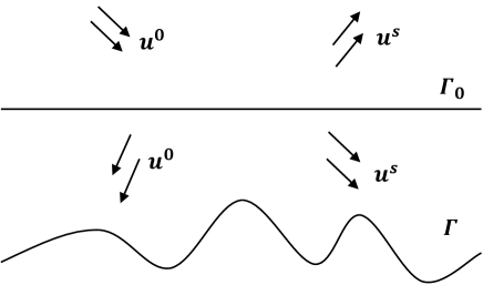
Consider the scattering problems with time-harmonic incident waves in the domain . In this paper, we assume that the incident wave is either a plane wave or a point-source wave. The reference wave is generated by the incident wave and the two-layered medium. The explicit expressions of the incident wave and its corresponding reference wave will be described later. Then the total field is the sum of the reference wave and the scattered wave , where satisfies the following Helmholtz equations
| (2.1) |
Moreover, we assume the total field satisfies the following boundary conditions on the interface , i.e.,
| (2.2) |
where ’+/-’ denote the limits from and , respectively. Furthermore, the boundary condition imposed on is given by on . Here, denotes one of the following two boundary conditions:
where , denotes the unit normal at pointing out of and denotes the normal derivative of with respect to .
To guarantee the uniqueness of the considered scattering problems, the scattered wave is required to satisfy a radiation condition. In contrast to the bounded obstacle scattering problems, which utilize the Sommerfeld radiation condition, needs to satisfy the so-called upward propagating radiation condition in with respect to , that is,
| (2.3) |
for some and , where with and is the free-space Green function for the Helmholtz equation with the wave number and with denotes the Hankel function of the first kind of order zero. We also need to satisfy the following boundedness condition
| (2.4) |
for some .
Furthermore, if is an impedance boundary, the scattered wave needs to satisfy that for some and some constant ,
| (2.5) |
for , where .
Now we describe the reference wave more specifically. The reference wave is the total field of the scattering problem in the two-layered medium without the rough surface and is generated by the incident wave . In this paper, we consider two types of incident waves, that is, the plane wave and the point-source wave.
First, we describe the reference wave in the case when the incident wave is the plane wave , where , . In this case, the reference wave is given by (see, e.g., (2.13a) and (2.13b) in [31] or Section 4 in [27])
| (2.6) |
with
where is the reflected direction, and where and are called the reflection and transmission coefficients, respectively, with and defined by
Here, with and is defined by
The definition of gives that
In particular, if , then is the transmitted direction with satisfying . It is easy to see that such reference wave satisfies the following conditions
| (2.7) |
Second, we describe the reference wave in the case when the incident wave is the point source wave , where if the source point and if the source point . In this case, the reference wave , where denotes the so-called two-layered Green function. Precisely, for any , the two-layered Green function is the solution of the following scattering problem (see page 17 in [31])
| (2.8) | ||||
| (2.9) | ||||
| (2.10) |
where for , denotes the Dirac delta distribution, denotes the unit normal on pointing into and denotes the jump across the interface . Here, (2.10) is called the Sommerfeld radiation condition. The explicit expression of is given by (see, e.g., [31, formula (2.27)])
| (2.11) |
where and are given by
| (2.12) |
| (2.13) |
Now the above scattering problems can be formulated as the following two boundary value problems (DBVP) and (IBVP) for the scattered wave .
Definition 2.1 ().
Let denote the set of functions such that and .
Dirichlet Boundary Value Problem (DBVP). Given , determine such that:
(i) is a solution of the Helmholtz equations in (2.1);
(ii) on ;
(iii) on ;
(iv) satisfies (2.4) for some ;
(v) satisfies the upward propagating radiation condition (2.3) in with the wave number .
Definition 2.2 ().
Let denote the set of functions satisfying , and satisfying that the normal derivative of defined by exists uniformly for on any compact subset of .
Impedance Boundary Value Problem (IBVP). Given , determine such that:
(i) is a solution of the Helmholtz equations in (2.1);
(ii) on ;
(iii) on ;
(iv) satisfies (2.4) for some ;
(v) For some and some constant , satisfies (2.5) for , where ;
(vi) satisfies the upward propagating radiation condition (2.3) in with the wave number .
Remark 2.3.
3 Properties of the Two-layered Green Function
In this section, we derive some properties of the two-layered Green function , which are useful for the investigation of the well-posedness of the considered boundary value problems and the convergence of the Nyström method in the following two sections. To this end, we give some notations. Define the angle if , where is given as in Section 2. For any , define and . Throughout the paper, the constants may be different at different places.
Let the two-layered Green function with be given as in Section 2. For any source point lying on the interface , due to the well-posedness of the scattering problem in a two-layered medium (see [2]), we can define the two-layered Green function as the unique solution that satisfies , in (in the distributional sense) and the Sommerfeld radiation condition (2.10), where denotes the fundamental solution of the Laplace equation in . Here, denotes the space of all functions such that for all open balls . Moreover, by the expression of the Hankel function given in [15, Section 3.5] and the expression of given in (2.11), it is clear that for any , also satisfies .
Let with . For any , let . Using the following integral representation of Hankel function (see [14, formula (2.2.11)])
| (3.1) |
for , with , the formula (2.11) for can be written as
| (3.2) |
where is the half-space Dirichlet Green function for (see [6]) and is defined as
for with and where is given by
| (3.3) |
Further, with the help of (3.1), we write as
where is defined by
| (3.4) |
for
The following lemma presents the continuity properties of .
Lemma 3.1.
For any with , we have .
Proof.
Let be arbitrarily fixed. Our proof is divided into three parts.
Part 1: we prove that is continuous at . Denote the ball centered at with radius by . Choose the cutoff function such that
with being a fixed number. Let . Then we have
For any and , we can easily verify that for some constant . Furthermore, for any and , we can easily prove that
| (3.5) |
Let be a bounded domain with -boundary . By the well-posedness of the scattering problem in a two-layered medium (see [2]) and the interior regularity of the elliptic equation (see [19, Sections 6.2 and 6.3]), it follows that for ,
| (3.6) |
for some constants , which implies that
| (3.7) |
Similarly to the above derivations, we can also obtain that for ,
| (3.8) |
Thus by using (3.7), (3.8) and (3.5), we can deduce that is continuous at . Hence is continuous at due to the fact that .
Part 2: we prove that is continuous at . To do this, we utilize the estimates of the elliptic equation. Choose the cutoff function such that
with a fixed number . Let , where is given as in Part 1. Then we have
By the Gagliardo-Nirenberg-Sobolev inequality (see [19, Theorem 1 in Section 5.6.1]), it follows that for any and any ,
for some constant , where satisfies (it is clear that ). This, together with (3.6), implies that for any and any ,
| (3.9) |
Similarly, it follows that for any and ,
| (3.10) |
It is easy to see that with is the solution of the following problem
Then it can be deduced from [20, Theorem 9.15] that
for any and . Furthermore, applying the Sobolev inequality given in [19, Theorem 6 in Section 5.6.3], Lemma 9.17 in [20] and the inequality (3.9), we obtain that for any and , with
for some constants . Similarly, we can apply [20, Lemma 9.17] and the inequality (3.10) to obtain that for any and ,
| (3.11) |
for some constant . Hence, by using the formulas (3.11) and (3.5) and the fact that , we have that is continuous at . This, together with the definitions of and , implies that is continuous at .
Part 3: we prove that is continuous at . It is known from [31, (2.28)] that for with . It was also proved in [27, Remark 3.5] that for any and for any . Thus it follows that for any with . This, together with the facts that for any with and (see the result in Part 1), implies that for any . Hence, we can apply the result in Part 2 to obtain that is continuous at .
Therefore, the proof is complete due to the arbitrariness of . ∎
Remark 3.2.
By Lemma 3.1, can be extended as a function in and can be extended as a function in .
The following lemma gives the asymptotic properties of .
Lemma 3.3.
Assume and let be an arbitrary fixed number. Suppose that and for and suppose that with for with . Then we have the asymptotic behaviors
where , satisfy
uniformly for all and . Here, the constant is independent of and but dependent of .
Proof.
The statement of this lemma is a direct consequence of the following asymptotic behaviors of the Hankel function (see (3.105) in [15])
∎
The following lemma provides the uniform far-field asymptotics of some functions relevant to the two-layered Green function , which are mainly based on the work [27].
Lemma 3.4.
Assume and let be an arbitrary fixed number. Suppose that and for and suppose that with for . Define
and
Then we have the following statements.
(i) For , we have the asymptotic behaviors
where and are given by
and where and satisfy the estimates
uniformly for all and ,
uniformly for all and , and
uniformly for all and . Here, the constant is independent of and but dependent of .
(ii) For , we have the asymptotic behaviors
where and are given by
and where and satisfy the estimates
uniformly for all and . Here, the constant is independent of and but dependent of .
Proof.
With the aid of the above lemmas and remarks, we have the following theorem on the asymptotic properties of and .
Theorem 3.6.
Assume that with . Let and . Define and . Then we have the following statements.
(i) If satisfy , then satisfies the inequalities
where the constant depends only on .
(ii) If satisfy and for some , then satisfies the inequalities
where the constant depends only on and .
Proof.
We only give the derivations on the estimates of and by using the asymptotic behaviors of and given in Lemma 3.4 and the continuity of given in Lemma 3.1. We omit the proof on the estimates of and , since these estimates can be similarly deduced by using the asymptotic behaviors of and given in Lemma 3.4 as well as the continuity of given in Lemma 3.1. Our proof is divided into the following three parts.
Part 1: we establish the estimates for when . In this part, we consider three steps.
Step 1.1: we prove that there exists some such that
| (3.12) |
for all with , where is a constant depending only on .
By taking the substitution in (3.3), can be rewritten as
for . This, together with Remark 3.5, implies that for ,
where with . Then it follows from Lemma 3.4 that
| (3.13) |
for , where satisfies
| (3.14) |
uniformly for all ,
| (3.15) |
uniformly for all , and
| (3.16) |
uniformly for all , where is a constant depending only on . If , then we can apply (3.15) and (3.16) to obtain that there exists such that
| (3.17) |
Moreover, if , then we can apply (3.14) and the fact that to deduce that there exists such that
| (3.18) |
Here, the constants , in (3.17) and (3.18) depend only on . Hence, combining the estimates (3.17) and (3.18), we have that there exists such that
| (3.19) |
for all with , where the constant depends only on .
On the other hand, since , it follows from (3.13) that
| (3.20) |
for all , where is a constant depending only on .
Step 1.2: we prove that there exists some such that satisfies (3.12) for all with , where the constant depends only on .
For , we can write as
Then we obtain from Remark 3.5 that
Hence it follows from Lemma 3.4 that
| (3.21) |
for , where satisfies
uniformly for , where is a constant depending only on . This implies that there exists such that
| (3.22) |
for all with , where the constant depends only on .
On the other hand, similarly to Step 1.1, it follows from (3.21) that
| (3.23) |
for all , where is a constant depending only on .
Step 1.3: we prove that for any , there exists a constant depending on such that (3.12) holds for all satisfying and .
Recall that for and for . Then from the equation (2.12) and Remark 3.2, it follows that for some function defined in , we can write as for and for . Using the continuity property of given in Remark 3.2, it is clear that can be extended as a function in . Thus we have that for any , there exists a constant depending only on and such that for all satisfying and . This, together with the asymptotic properties of the Hankel function for small arguments (see [15] for the expression of ), implies that there exists a constant such that (3.12) holds for satisfying and .
From the discussions in Steps 1.1, 1.2 and 1.3, we obtain that satisfies (3.12) for all satisfying , where the constant depends only on .
Part II: we establish the estimates for when . In this part, we consider three steps.
Step 2.1: we prove that there exists some such that
| (3.24) |
for all satisfying , and , where is a constant depending only on and .
Suppose that satisfy and . Let with and . By the change of variable , can be written as
Then it follows from Remark 3.5 that
Hence using Lemma 3.4, we obtain that
| (3.25) |
for , , where satisfies
| (3.26) |
uniformly for all and ,
| (3.27) |
uniformly for all and , and
| (3.28) |
uniformly for all and , where is a constant depending only on and .
If , then we can apply (3.26) and the fact that to obtain that there exists such that
| (3.29) |
for . Moreover, if , then we can apply (3.27) and (3.28) to deduce that there exists such that
| (3.30) |
Here, the constants , , in (3.29) and (3.30) depend only on and . Combining (3.29) and (3.30), we have that there exists such that
| (3.31) |
for all satisfying , and , where is a constant depending only on and .
On the other hand, since and , we obtain from (3.25) that
| (3.32) |
for all satisfying and , where is a constant depending only on and .
Hence, (3.31) and (3.32) give that (3.24) holds for all satisfying , and , where is a constant depending only on and .
Step 2.2: we prove that there exists some such that (3.24) holds for all satisfying , and , where is a constant depending only on and .
Suppose satisfy and . By (2.13) we can write as
This, together with Remark 3.5, implies that
where and . Then it follows from Lemma 3.4 that for and ,
| (3.33) |
where satisfies
uniformly for all and with and where is a constant depending only on and . Thus there exists such that
| (3.34) |
for , where is a constant depending only on and .
On the other hand, similarly to Step 2.1, by (3.33) we have
| (3.35) |
for satisfying and , where is a constant depending only on and .
Hence, it follows from (3.34) and (3.35) that satisfies (3.24) for all satisfying , and , where the constant depends only on and .
Step 2.3: we show that for any , there exists a constant depending on and such that (3.24) holds for satisfying , and .
Recall that for and for . By (3.4), we can write as , where is a function defined on and with . Using the continuity property of given in Remark 3.2, we obtain that can be extended as a function in . Thus we have that for any , there exists a constant depending only on such that for satisfying , and . This, together with the asymptotic properties of the Hankel function for small arguments, implies that there exists a constant such that (3.24) holds for satisfying , and .
Based on the analysis in Steps 2.1, 2.2 and 2.3, we obtain that satisfies (3.24) for all satisfying and , where the constant depends only on and .
Part III: we establish the estimates for and when .
Define
where and . Then by (3.2), it can be seen that for any , is the two-layered Green function satisfying the scattering problem (2.8)–(2.10) with for and for . Thus, by using the same analysis as in Parts I and II, we can directly obtain that
| (3.36) |
for all satisfying and that
| (3.37) |
for all satisfying and . Hence it follows from (3.36) that satisfies (3.12) for all satisfying , where the constant depends only on . Moreover, it can be seen from (3.37) that satisfies (3.24) for all satisfying and , where the constant depends only on .
Therefore, the proof is complete. ∎
Similar properties as in Theorem 3.6 have been established for the half-space Dirichlet Green function and the half-space impedance Green function (see [37, inequalites (8) and (24)]). Especially, we mention that satisfies the estimates (see [37, Formula ])
| (3.38) |
for with , where the constant depends only on .
Finally, as a direct consequence of (3.2), (3.38), Lemma 3.1 and Theorem 3.6, we can obtain the following theorem on the estimates of , which is crucial for this paper.
Theorem 3.7.
Assume that with . Let and . Define and . Then we have the following statements.
(i) If satisfy , then satisfies the inequalities
| (3.39) |
where the constant depends only on .
(ii) If satisfy and for some , then satisfies the inequalities
| (3.40) |
where the constant depends only on and .
4 The Well-posedness of the Problems (DBVP) and (IBVP)
In this section, we consider the well-posedness of the problems (DBVP) and (IBVP). In Section 4.1, we provide some a priori estimates of the first derivatives of relevant solutions. Then following the ideas in [7, 10, 37], we prove the uniqueness results for the problems (DBVP) and (IBVP) in Sections 4.2 and 4.3, respectively. Furthermore, the existence results for the problems (DBVP) and (IBVP) are given in Sections 4.4 and 4.5, respectively.
4.1 The Derivative Estimates
If satisfies the conditions (i)–(iv) of the problem (DBVP) with , we can apply the standard elliptic regularity estimate [20, Theorem 8.34] to deduce that . Let denote the space of essentially bounded functions defined on . Then the following lemma presents the local regularity estimate of solutions to the Laplace equation.
Lemma 4.1 (Lemma 2.7 in [9]).
If is open and bounded, , and (in a distributional sense), then and
where is an absolute constant and .
Using the formula (2.4) and Lemma 4.1 with to be a sufficiently small ball centered at , we can obtain the following Theorem. See [10, formula (3.1)] for a similar result.
Theorem 4.2.
If satisfies the conditions (i)–(iv) of the problem (DBVP) or satisfies the conditions (i)–(iv) of the problem (IBVP), then there exists some such that
for all .
Moreover, by similar arguments as in the proof of [10, Theorem 3.1], we have the following estimates on the solution satisfying the conditions (i)–(iii) of the problem (DBVP) with .
Theorem 4.3.
If satisfies the conditions (i)–(iii) of the problem (DBVP) with , then we have that for some positive constant C,
for , where and with .
Proof.
The statement of this theorem can be deduced by using the proof of [10, Theorem 3.1] with a minor modification, since the main difference between the proof of this theorem and that of [10, Theorem 3.1] lies in the presence of the interface . To be more specific, the minor modification is that we only need to replace and used in the proof of [10, Theorem 3.1] by and , respectively, where is given as in the proof of [10, Theorem 3.1]. Here, we note that by choosing such replacement, the ball of radius with center at is contained in for any . ∎
4.2 The Uniqueness Result of the Problem (DBVP)
In this subsection, we prove the uniqueness of the problem (DBVP) with the help of the a priori estimates given in Section 4.1. We introduce some notations, which will be used in the rest of this paper. For and with , define and . For , define . Given an open set and , let () denote the (distributional) derivative and we abbreviate (that is, the normal derivative of ) as .
The following theorem presents an inequality for the solution of the problem (DBVP) with , which plays a crucial role in the proof of the uniqueness result.
Theorem 4.4.
Assume . Let be the solution of the problem (DBVP) with . Let and with . Then we have
| (4.1) |
where denotes the unit normal on pointing out of and where and are given by
Here, is a constant depending only on .
Proof.
Define for and let be the boundary of . Let denote the outward unit normal to . Noting that Rellich’s type identity , we find, by applying the divergence theorem in , that
| (4.2) |
where , and are given by
Furthermore, by using the identity in the domain and the fact that , we obtain that
| (4.3) |
where
It follows from Theorems 4.2 and 4.3 that the integral is well-defined and thus we have
| (4.4) |
By the boundary condition of , we have on . Thus we can deduce that and on . This, together with the fact that on , implies that
Therefore, from the above discussions, it follows that (4.1) holds. This completes the proof. ∎
Remark 4.5.
Next, we show that the solution of the problem (DBVP) with can be written as an integral relevant to its normal derivative on . For this purpose, we define for and introduce the following definition.
Definition 4.6.
Given a domain and , call a radiating solution of the Helmholtz equation in if in and
| , | |||
as , uniformly in .
Theorem 4.7.
Let be the solution of the problem (DBVP) with . Then
| (4.6) |
where denotes the unit normal on pointing out of .
Proof.
First, we consider the case when . Let and define the domain
| (4.7) |
where denotes the ball centered at with radius small enough such that . Since , it follows from Green’s theorem that
where denotes the outward unit normal on . By the mean value theorem and the formula (2.11), we obtain that
By the estimates in (3.39) as well as Theorems 4.2 and 4.3, it follows that
| (4.8) |
Using the transmission boundary conditions of and on the interface , we obtain
where ’+/-’ are the limits given as in (2.2). With the help of Theorems 3.7 and 4.2, we can apply Green’s theorem in the domain with to obtain that
From the definition of the two-layered Green function given in (2.8)–(2.10) and the estimates in (3.40), together with the symmetry property for with (see [31, (2.28)]), we have that is a radiating solution of in and that and belong to . Note that satisfies the upward propagating radiation condition (2.3) in . Hence we can employ [10, Lemma 2.1] to obtain
| (4.9) |
From the facts that on and , together with (4.5) and the estimates in (3.39), we can deduce that
By using the above discussions, we obtain that the formula (4.6) holds for .
Lemma 4.8 (Lemma A in [10]).
Suppose that and that, for some nonnegative constants , , , and ,
and
where, for ,
Then and
The following lemma gives some properties of the two-layered Green function, which will be used in this subsection, in Section 4.3 and in Appendix A.
Lemma 4.9.
Assume with . Define and . Then we have the following statements.
(i) For , there hold , , and .
(ii) Let . There hold
| (4.10) |
for all satisfying , and , where the constant depends only on .
(iii) Let be a bounded domain such that . Then we have that and () satisfy the Sommerfeld radiation condition (2.10) uniformly for all and .
Proof.
The statement (i) can be directly deduced by the expression (2.11) of G(x,y) and Lebesgue’s dominated convergence theorem.
For the statement (ii), we only derive the estimate for , since the estimate for can be deduced in a similar manner. We choose and in such that , and . Then by the expression (2.11) of , together with the integral representation of Hankel function given in (3.1), it can be verified that , , satisfies the Helmholtz equations in with the wave numbers , respectively, and satisfies the transmission boundary condition on , i.e.,
for . Thus, taking such that , we obtain that , satisfies in in the distributional sense with and , where is a ball with center and radius . Hence, using Lemma 4.1 for in and applying the statements (i) and (ii) in Theorem 3.7, we obtain
where and the constant depends only on . This completes the proof.
Finally, by employing similar arguments as in the proofs of Theorems 2.1 and 2.14 in [27], we can use patient calculations to obtain that the statement (iii) holds true. ∎
The following lemma has been proved in [9].
Lemma 4.10 (Lemma 6.1 in [9]).
Let . If and is defined by (2.3), then , and are in for all and
| (4.11) | |||
| (4.12) |
Now, we assume that > and that is the solution of the problem (DBVP) with . We proceed to show that vanishes on . Let and . Then we can set in the formula (4.1) to obtain that
where and . Let be defined by
| (4.13) |
By employing Lemma 3.1, (3.40) and the property of given in Remark 4.5, it can be derived that for all . On the other hand, it is easy to see from (2.8), (3.40) and the statement (iii) of Lemma 4.9 that is a radiating solution of in for all . Thus, in view of the equivalence of the statements (ii) and (iv) in [9, Theorem 2.9], satisfies (2.3) with and for every . Hence, by employing (4.11), we have , where
By applying Green’s theorem in the domain and in the domain , we can use the conditions (ii) and (iii) in the problem (DBVP) to find that , where
Thus, from the above discussions, we can derive
Set
and . Then for all ,
By the formulas (4.6) and (4.13) and the estimates (3.40) and (4.10), we obtain that
where the constant is independent of but dependent on and where and are defined by
These lead to
where . Hence, there exists a constant such that for all ,
Combining this with (4.5) and the fact that (see Remark 4.5), we can apply Lemma 4.8 to conclude that , which is equivalent to , and that for all ,
| (4.14) |
For with , we deduce by (4.6) and (3.40) that
where
Thus, as with , uniformly in . Hence by Theorems 4.2 and 4.3 as well as Lemma 4.1, we have as , . Therefore, it follows from (4.14) that on .
In conclusion, based on the above discussions and Theorem 4.7, we establish the following theorem on the uniqueness of the problem (DBVP).
Theorem 4.11.
For every , there exists at most one solution that satisfies the boundary value problem (DBVP) under the assumption .
Remark 4.12.
In the case , it can be seen from [25, Example 2.3] that when the rough boundary is a planar surface, there exist some wave numbers and such that the problem (DBVP) with has a nontrivial solution.
4.3 The Uniqueness Result of the Problem (IBVP)
Theorem 4.13.
Let be the solution of the problem (IBVP). Then
| (4.15) |
where denotes the unit normal on pointing out of .
Proof.
First, we consider the case when . Let and let the domain be given as in (4.7), where denotes a ball centered at with radius small enough such that . By applying Green’s theorem in the domain and letting , it follows that
| (4.16) |
where ’-’ in the third integral of the above formula is the limit given as in (2.2). With the help of Theorems 3.7 and 4.2, we can apply the same arguments as in the derivations of (4.8)–(4.9) to obtain that
and that for ,
Thus we can obtain the formula (4.15) by letting in the formula (4.16).
In the rest of this subsection, with a slight abuse of notations, we will redefine , , , , , , and . Applying Green’s theorem in the domains and with and using the conditions (ii) and (iii) in the problem (IBVP), we can immediately obtain the following lemma.
Lemma 4.14.
Set . Let satisfy the problem (IBVP) with . Then
where
| (4.17) |
Now we give the uniqueness of the problem (IBVP).
Theorem 4.15.
Suppose that and . If with on , then the problem (IBVP) has at most one solution for every .
Proof.
Let satisfy the problem (IBVP) with . We need to show that in . Let and define by
| (4.18) |
By utilizing the estimates of in (3.40) and the fact that , it can be derived that for all . On the other hand, it follows from (2.8), (3.40) and the statement (iii) of Lemma 4.9 that is a radiating solution of in for all . Thus, in view of the equivalence of the statements (ii) and (iv) in Theorem 2.9 in [9], satisfies (2.3) with and for every .
Let and set
Then by (4.12) in Lemma 4.10, , so that, by (4.17) and the fact that for , we have
Let . Then
Set
It follows from the formulas (4.15) and (4.18) and the estimates (3.40) and (4.10) that
This leads to
Hence, the above analysis gives that
By employing Lemma 4.8, we obtain that for all ,
| (4.19) |
From (2.4) and the fact that , we obtain that . This, together with Theorems 4.13 and A.3, implies that for every . Thus , which yields that as for . Choose a cutoff function such that with for and for . Let and be given by (4.15) with , where the density is replaced by and , respectively. Thus for . From Theorems A.1 (iii) and A.2 (iii), we have that there exists some constant such that for all , as . Moreover, it follows from the definition of and Theorem 3.7 that there exists some constant such that
Hence, by (2.5) we obtain that as . Consequently, from (4.19) we have on . This, together with (4.15), implies that in . Therefore, the proof is complete. ∎
4.4 The Existence Result of the Problem (DBVP)
For , the integrals
| (4.20) | ||||
| (4.21) |
are called the double- and single-layer potentials, respectively. Here, denotes the unit normal on pointing out of . The properties of the double-layer potential (4.20) and the single-layer potential (4.21) are summarized in Appendix A.
We introduce a function in the form of a combined double- and single-layer potential, i.e.,
| (4.22) |
where , is a constant. From the statements (i), (iii) and (v) in Theorem A.1 and the statements (i), (iii) and (iv) in Theorem A.2, the potential satiefies the conditions (i), (ii), (iv) and (v) of the problem (DBVP) with . Furthermore, by the statement (ii) in Theorem A.1 and the statement (ii) in Theorem A.2, satisfies the condition (iii) of the problem (DBVP) only if is the solution of the following boundary integral equation
| (4.23) |
Thus we get the following result.
Theorem 4.16.
Define by
| (4.24) |
By parameterizing the equation (4.23), we obtain the following integral equation problem: find such that
| (4.25) |
where . Define the kernel by
| (4.26) |
with . Using this kernel, define the integral operator by
for . Then the equation (4.23) can be written as
where denotes the identity operator on . Here, we use the subscript to indicate the dependence of the kernel and the operator on the function .
Since with is an integral over the unbounded interval , is not a compact operator on . Thus it is impossible to use the Riesz-Fredholm theorem to establish the solvability of the integral equation (4.25). To overcome this difficulty, we follow the approach in [37]. The following theorem presents the uniqueness of the integral equation (4.23).
Theorem 4.17.
If and , then the integral equation (4.23) has at most one solution in .
Proof.
Suppose that satisfies
| (4.27) |
It suffices to prove that . Define by with . Let with be the combined double- and single-layer potential with the density function , that is,
Then satisfies (4.23) with . Hence, it follows from Theorem 4.16 that satisfies the problem (DBVP) with , so that, by Theorem 4.11, in . Furthermore, let and be defined as in the equations (A.6) and (A.2), respectively. Then it follows that on . By the statements (ii) and (iv) in Theorem A.1 and the statement (ii) in Theorem A.2, we have the following jump relations
| (4.28) |
which implies that and . Hence
| (4.29) |
For , we define . Define
| (4.30) | |||
| (4.31) |
It can be observed that (resp. ) if and only if (resp. ).
Let be defined as
| (4.32) |
for . Let be the unit normal to pointing out of and let be the unit normal to pointing out of . Define
It is clear that and for . This, together with (4.29), (4.27), the boundary condition on as well as Theorem A.3, implies that . Thus, by Theorems A.4 and A.5, satisfies the condition (iv) of the impedance problem (IP) in [37, Section 2]. Then by combining the statements (i), (iii) and (v) in Theorem A.1 and the statements (i), (iii) and (iv) in Theorem A.2, satisfies the conditions (i), (iii) and (v) of the impedance problem (IP) in [37]. Hence, based on the above discussions, satisfies the impedance problem (IP) in [37] with , , and with the wave number and the boundary data . Choose so that for some . Then by [37, Theorem 4.7], in , which implies that in . Then the jump relations in (4.28) give that . Therefore, the proof is complete. ∎
In the rest of this subsection, we assume that and . Now we utilize Theorem B.1 to prove the existence of the integral equation (4.25). We use the notations defined in Appendix B. For some and , we define by
Let . By Theorem 4.17, is injective for all , where is defined by (B.1) and is the identity operator on . Then for all , where . By Lemma B.2 (i), , and for all satisfies
By the statements (i) and (ii) in Lemma B.3, is sequentially compact in . Let and such that . Choose a periodic function satisfying for and let . Then it yields that
This, together with Lemma B.3 (ii), implies that . Since , where is the period of , and , it follows from Theorem 2.10 in [8] that (B.4) holds. By the above discussions, satisfies all the conditions of Theorem B.1 and thus we obtain the following results.
Theorem 4.18.
By combining Theorems 4.11, 4.16, 4.17, 4.18, A.1 (iii) and A.2 (iii), we arrive at the following theorem on the well-posedness of the problem (DBVP).
Theorem 4.19.
Assume and . Then for every and , the problem (DBVP) has exactly one solution in the form
Here, the density function is the unique solution of the integral equation
where is bijective (and thus boundedly invertible) in . Moreover, for some constant depending only on and ,
for all and .
4.5 The Existence Result of the Problem (IBVP)
In this subsection, we seek a solution in the form of the single-layer potential
| (4.33) |
for some . Using the statements (i) and (iii) in Theorem A.2, we obtain satisfies the conditions (i), (ii) and (iv) of the problem (IBVP) with . With the aid of Theorem A.5, we have that satisfies the condition (v) of the problem (IBVP) for any . Thus, by Theorem A.2 (ii), the single-layer potential (4.33) is a solution of the problem (IBVP) provided satisfies the following integral equation
| (4.34) |
Hence, we obtain the following theorem.
Theorem 4.20.
Let and be given as in (4.24) and let be given by
| (4.35) |
By parameterizing the integral in (4.34), we have the following integral equation problem: find such that
| (4.36) |
where and . Define the kernel by
| (4.37) |
where and . Using this kernel, define the integral operator by
for . Then the equation (4.34) can be written as
where denotes the identity operator on . Here, we use the subscript to indicate the dependence of the kernel and the operator on the functions and .
Using Theorem 4.15 for the uniqueness of the impedance problem (IBVP), we can establish the following uniqueness result for the integral equation (4.34).
Theorem 4.21.
Suppose that and . If with on , then the boundary integral equation (4.34) has at most one solution in .
Proof.
Suppose satisfies
We only need to prove that .
Define by , and let in be the single-layer potential with the density , that is,
Then satisfies (4.34) with , so that, by Theorem 4.15, in . Furthermore, by Theorem A.2 (ii),
| (4.38) |
where and are defined as in the equations (A.2) and (A.6), respectively. Thus, on . This implies that on , where is given as in (4.30) and is defined in the same way as in (4.32). Moreover, let be given as in (4.31). By the statements (i)–(iv) of Theorem A.2, satisfies the problem (P) in [10, Section 2] with and and with the boundary data on . Hence, by Theorem 3.4 in [10], it follows that in , which implies that in . Therefore, by (4.38) we obtain . The proof is now completed. ∎
Now we are going to prove the existence of the integral equation (4.34). We will use Theorem B.1 and use the notations in Appendix B. For some , and some function such that as , let be defined by
Note that . Conversely, given , it holds that provided and for all . We have the following existence result for the integral equation (4.34).
Theorem 4.22.
Proof.
Let . It follows from Theorem 4.21 that is injective for all , where is defined by (B.1) and is the identity operator. Moreover, for all . By Lemma B.2 (ii), and satisfies (B.3). From the statement (i) in Lemma B.3 and the statements (i) and (ii) in Lemma B.4, is -sequentially compact in . Let , and such that . For each , choose and so that and are periodic with the same period and , for . Then and , , , so that, by Lemma B.4 (ii), . Since , where is the period of and and where , it follows from [8, Theorem 2.10] that the condition (B.4) holds. Thus satisfies all the conditions in Theorem B.1. Therefore, the statement of this theorem follows from Theorem B.1. ∎
By combining Theorems 4.15, 4.20, 4.21, 4.22, A.1 (iii) and A.2 (iii), we obtain the following result on the well-posedness of the problem (IBVP).
Theorem 4.23.
Assume and with . Suppose that for some , for all . Then for every and with uniformly continuous on , the problem (IBVP) has exactly one solution in the form
Here, the density function is the unique solution of the integral equation
where is bijective (and thus boundedly invertible) in . Moreover, if , then for some constant depending only on , and ,
for all , and with defined in terms of by (4.35).
5 The Nyström Method for the Problems (DBVP) and (IBVP)
In this section, motivated by [29], we present the Nyström method for numerically solving the problems (DBVP) and (IBVP), based on the integral equations (4.23) and (4.34). Nyström methods have been extensively studied for computing solutions of integral equations on bounded curves (see, e.g., [15]). Moreover, this kind of methods was extended in [29] to solve integral equations on unbounded domains.
For , define the boundary integral operators
For , we write and for . For the functions , we define the parameterized functions in terms of (4.24) and (4.35). Then the above three integral operators can be parameterized as
for , respectively, where the kernels , and are given by
Next, we rewrite the operators , and . Let denote the Hankel function of the first kind of order and let and denote the Bessel function and the Neumann function, respectively, of order (see [15]). According to (2.11), the expansion (3.98) in [15] for the Neumann functions, and the properties of Hankel functions and for , the kernels and have the representations
| (5.1) | |||
| (5.2) | |||
| (5.3) |
where and () are given by
| (5.4) | |||
| (5.5) | |||
| (5.6) | |||
| (5.7) | |||
| (5.8) | |||
| (5.9) |
where , , and . We note from (2.12) that for . Then using the formulas (3.97) and (3.98) in [15], we can deduce that the diagonal terms for , and
for , where denotes the Euler constant.
Let denote the cut-off function satisfying for and satisfying that for , for and for . Then , and can be written as
where and are given by
for . In particular, we set for all and
In the following two subsections, we will give the convergence analysis and the numerical implementation of our Nyström method.
5.1 Convergence Analysis
Set the step length for and set for . It follows from [29] that we can approximate the integral operators and by and , respectively, which are given by
| (5.10) |
for . Here, is given by
with
for and
Using the discretization operators and , we approximate the integral equations (4.25) and (4.36) by
| (5.11) |
and
| (5.12) |
respectively. Here, the functions denote the solutions of the approximate systems (5.11) and (5.12), respectively.
Let and be the solutions of the equations (4.25) and (4.36), respectively. In the rest of this subsection, we estimate the error terms and by applying Theorem 3.13 in [29]. To this end, we define the condition for any kernel function with and .
For , we say that satisfies if
where , , and there exist constants and such that for all with , we have
| (5.13) |
and
| (5.14) |
For , we denote by the Banach space of all functions whose derivatives up to order are bounded and continuous on with the norm defined by
where .
To give the convergence of Nyström method, we should introduce some function spaces for the functions and . For , and , we define the function space
For , and , let
Note that and are different from and . It can be seen that and for if , , for some .
Theorem 5.1.
Proof.
Let and . The proof is divided into two parts.
First, we establish the estimates of in (5.13). Let . Then it can be seen that . By utilizing the power series expansions of Bessel functions of the first kind (see [30, equation (10.2.2)]), we have for . Note that (see [1, statement (7.1.36) in Section 7.1.3]) and is uniformly bounded for all with (see [1, formulas (7.1.32) and (7.1.33) in Section 7.1.3]). Consequently, from the definition of and the formulas (5.4) and (5.6), it follows that with
| (5.15) |
for all with , where the constant depends only on .
Second, we establish the estimates of in (5.13). From (5.5) and (5.7), we write , as
and
By using as well as the power series expansions of Bessel functions [30, equations (10.8.1) and (10.8.2)], and can be rewritten as
where . Here, is the Euler constant and denotes the Gamma function (see [30, (5.2.1)]). Consequently, from the fact that and the analyticity of the power series involved in the above two formulas for , we obtain that for . By utilizing the expression (2.12) of , it follows that and has the form for some function with . Thus for any and with , is bounded in for with . By choosing , we obtain that for any with ,
for any satisfying and , where is a constant depending only on . Hence, combining the above analysis and the definition of , we deduce that and
| (5.16) |
for all with , where the constant depends only on .
Third, we show that satisfies (5.14). In fact, it is clear from Theorem 3.7 (i) that for ,
This, together with the regularity estimates for solutions to elliptic partial differential equations (see [20, Theorem 3.9]) and the symmetry property for with (see [31, (2.28)]), implies that for any , and with ,
for all satisfying and , where the constant depends only on . Furthermore, since , we have that and belong to . Thus it follows from the definition of the kernel in (4.26) that
| (5.17) |
for any satisfying , where the constant depends only on .
Part 2: we consider the kernel . With a slight abuse of notations, define
and
for . For and given in this part, since , we can use similar arguments as in Part 1 to obtain that and that the estimates (5.15) and (5.16) also hold for and , where the constant depends on . Moreover, by the definition of in (4.37), the estimates in (5.17) also hold for , where the constant depends only on . Therefore, the proof is complete. ∎
As a direct consequence of Theorems 4.19, 4.23 and 5.1, we can apply [29, Theorems 2.1 and 3.13] to obtain the following two theorems on the convergence of our Nyström method.
Theorem 5.2.
5.2 Numerical implementation
Now we describe the numerical implementation of our Nyström method. With the benefit of the convergence results given in Theorems 5.2 and 5.3, the main part of our method is to numerically solve the discretized equations (5.11) and (5.12) instead of solving the equations (4.25) and (4.36). For the integrals arising in (5.11) and (5.12), we truncate the infinite interval into a finite interval with satisfying , where is given as in Section 5.1. That is, the integral operators , and defined in (5.10) are approximated by
for , and , respectively. Then by using these approximations and choosing for in (5.11) and (5.12), the equations (5.11) and (5.12) are reduced to two finite linear systems which can be solved to obtain the approximate values of the density functions and at the points (). Finally, by using the relations (4.24) and (4.35) and the formulas (4.22) and (4.33), we can apply the trapezoidal rule to calculate the approximate values of the scattered wave at any points in the domain . It is worth mentioning that in our method, we use the approach given in [31, Section 2.3.5] to compute the two-layered Green function with high accuracy. Moreover, to accelerate our algorithm, we divide the matrices involved in the above linear systems into several matrices with smaller sizes and compute these small matrices in parallel.
In the rest of this subsection, numerical experiments will be carried out to demonstrate the feasibility of our Nyström method for the problems (DBVP) and (IBVP). In all of the following examples, we set . For the problem (DBVP), the parameter involved in relevant integral equations is set to be .
To investigate the performance of our method, we will choose a sampling set in with finite points and define the following relative error: for any wave field ,
where is a vector consisting of the approximate values of at the points in by using our Nyström method and denotes the infinity norm for any function defined in .
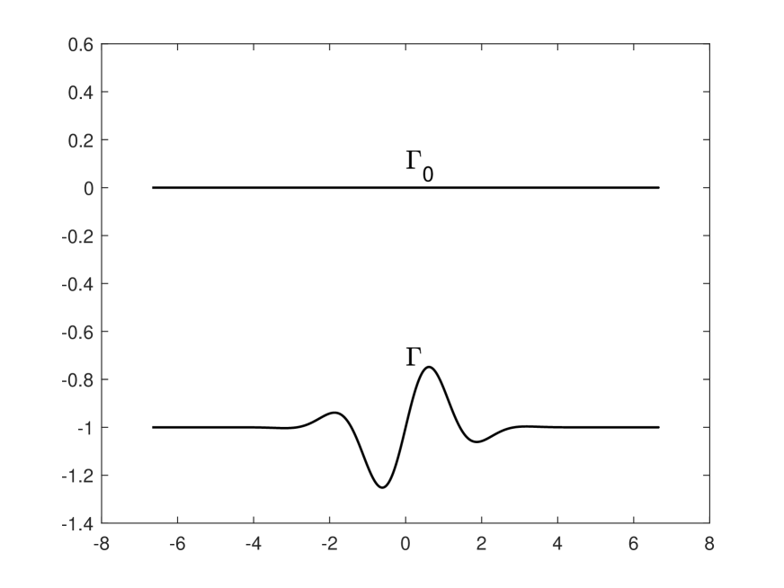
Example 1. Consider the rough surface with (see Figure 5.1 (a))
We choose the wave numbers , and choose to be the set of points uniformly distributed on the line segment . In the first case, we consider the problem (DBVP). Let be the solution of the problem (DBVP) with the boundary data , where denotes the two-layered Green function at the source point . It is easily verified that in and thus the exact values of can be obtained by using the approach given in [31, Section 2.3.5]. The second column of Table 5.1 presents the relative errors of our method with . In the second case, we consider the problem (IBVP). We choose . Let be the solution of the problem (IBVP) with the boundary data , where is given as above. It is also easily verified that in and thus the exact values of can also be obtained as in the first case. The third column of Table 5.1 presents the relative errors of our method with .
| (DBVP) | (IBVP) | ||
|---|---|---|---|
| N | |||
| 8 | 0.0015 | 0.0043 | |
| 16 | 3.3423e-06 | 8.6324e-06 | |
| 32 | 8.8875e-07 | 5.2844e-07 | |
| 64 | 9.8288e-08 | 1.8623e-07 |
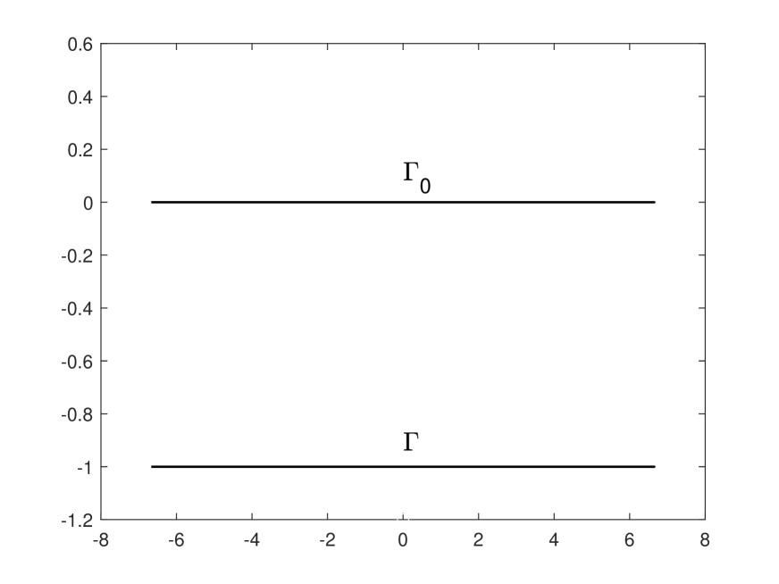
Example 2. Consider the rough surface as the flat plane (see Figure 5.1 (b)). We choose the wave numbers , and choose to be the set of 100 points uniformly distributed on the line segment . We set . For such , let , , , the plane wave and the reference wave be given as in Section 2. Here, note that since , then with satisfying . Further, let be the reflection of about the -axis. In the first case, we consider the problem (DBVP). Let be the solution of the problem (DBVP) with the boundary data . Then it can be seen from Section 2 that is the total field of the scattering problem (2.1)–(2.4) with the sound-soft boundary and with the incident wave given by . Moreover, since the rough surface is a plane, the total field has the analytical expression (see [14, Section 2.1.3])
| (5.18) |
with satisfying the system of linear equations
which is due to the transimssion conditon (2.2) of on and the Dirichlet boundary condition on . Thus we can obtain the exact values of by the above formulas. The second column of Table 5.2 presents the relative errors with , where the approximate values of are obtained by applying our method to the numerical computations of . In the second case, we consider the problem (IBVP). We choose on . Let be the solution to the problem (IBVP) with . Then it can be seen from Section 2 that is the total field of the scattering problem (2.1)–(2.5) with the impedance boundary and with the incident wave given by . Similarly to the first case, has the analytical expression (5.18) with satisfying the system of linear equations
which is due to the tramsimsion condition (2.2) of on and the impedance boundary condition on . Thus we can also obtain the exact values of . The third column of Table 5.2 shows the relative errors with , where the approximate values of are obtained by applying our method to the numerical computations of .
| (DBVP) | (IBVP) | ||
|---|---|---|---|
| N | |||
| 8 | 2.0781e-04 | 4.4780e-05 | |
| 16 | 1.0260e-04 | 2.4418e-05 | |
| 32 | 6.0844e-05 | 1.4069e-05 | |
| 64 | 3.7765e-05 | 8.4220e-06 |
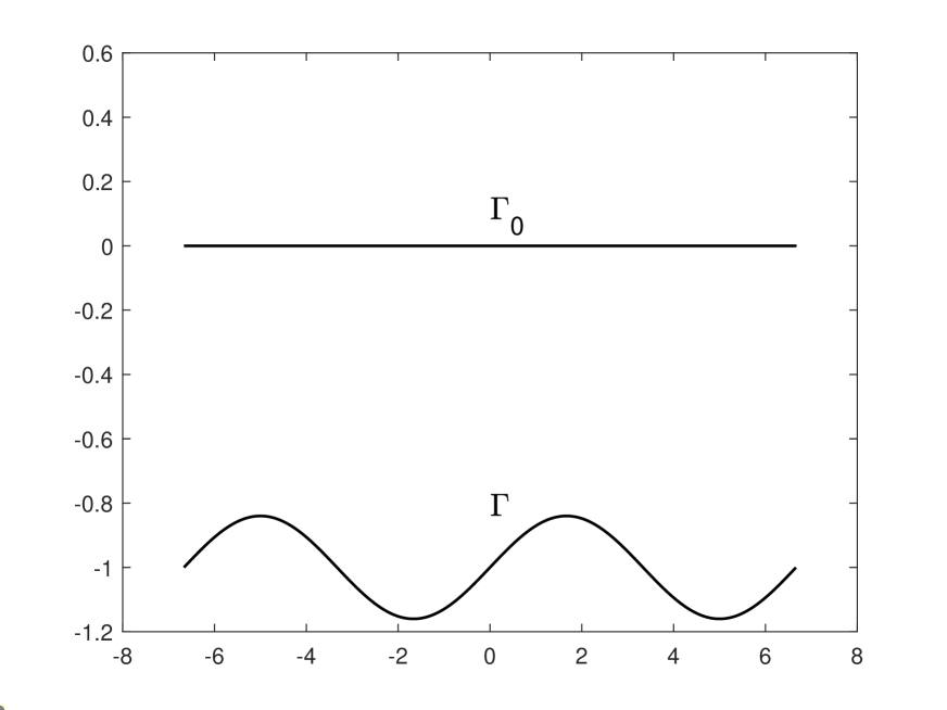
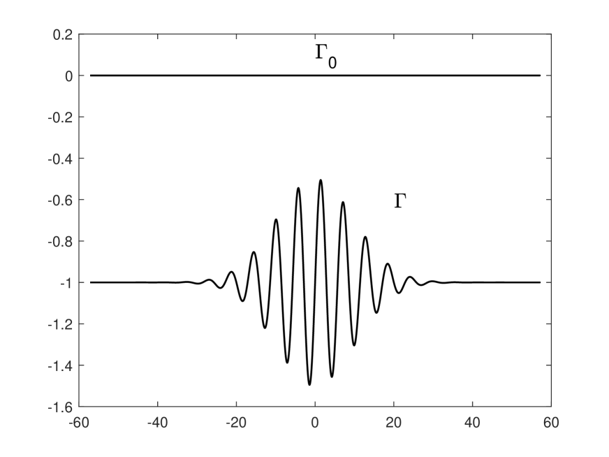
Example 3. Consider the rough surface to be a periodic curve with (see Figure 5.1 (c))
We choose the wave numbers and choose to be the set of points uniformly distributed on the line segment . Let the plane wave and the reference wave be given as in Section 2, where is chosen to be . Let be the solution of the problem (DBVP) with the boundary data and let be the solution of the problem (IBVP) with , where we choose on . Then similarly to Example 2, (resp. ) is the total field of the scattering problem (2.1)–(2.4) with the sound-soft boundary (resp. the scattering problem (2.1)–(2.5) with the impedance boundary ), where the incident wave is given by . In this example, we compute the approximate values of and by our method, which are obtained in a same way as in Example 2.
Note that the rough surface and for have the same period in -direction. Thus, to test the performance of our method, we model the considered scattering problems as the quasi-periodic scattering problems (see, e.g., [13]) and then use the finite element method with the technique of perfectly matched layer (PML) to compute the PML solutions and , which are the approximations of and , respectively. To be more specific, we use the PML technique given in [13] with the following settings. The problem is solved in the domain . The PML layer is chosen to be with the thickness of the PML layer as suggested in [13, Section 6]. The number of nodal points is chosen to be with using uniform mesh refinement. The finite element method with the PML technique is implemented by the open-source software freeFEM++ (see [22]). By the above approach, we can compute the approximate values of and in the domain . Moreover, the approximate values of and in the domain can be obtained by using the quasi-periodic properties of and (see [13]), i.e.,
for any in .
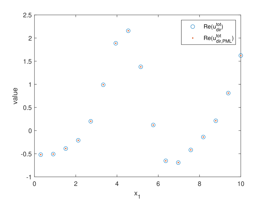
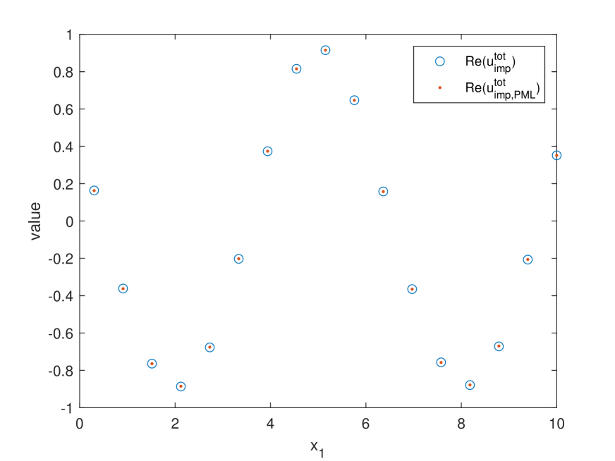
Table 5.3 shows the approximate values of and with by using our Nyström method as well as the approximate values of and by using the finite element method with the PML technique, where is chosen to be the point . Figure 5.2 presents the real parts of the approximate values of and by using our Nyström method with (blue circles) as well as the real parts of the approximate values of and by using the finite element method with the PML technique (orange dots), where we choose to be some discrete points on the segment line .
| (DBVP) | (IBVP) | ||||
| N | |||||
| 8 | 1.62243876 | 0.57170715 | 0.35175005 | 0.84347716 | |
| 16 | 1.62236304 | 0.57170811 | 0.35174104 | 0.84346688 | |
| 32 | 1.62228626 | 0.57168368 | 0.35173401 | 0.84346096 | |
| 64 | 1.62224382 | 0.57167564 | 0.35172998 | 0.84345808 | |
| PML solution | 1.62194914 | 0.56924364 | 0.35164894 | 0.84255734 | |
Example 4. Consider the rough surface (see Figure 5.1 (d)) with
We choose the wave numbers , and choose to be the set of points uniformly distributed on the line segment . Let with be the incident direction. Similarly to the reference wave defined in Section 2, we introduce the reference wave that is generated by the incident plane wave propagating in the lower half space and that satisfies the Helmholtz equations as well as the transmission boundary condition in (2.7). Similarly to the Fresnel formulas given in (2.6), is given by
| (5.19) |
where and with satisfying and where the coefficient functions and are defined by
In the first case, we consider the problem (DBVP). Let be the solution of the problem (DBVP) with the boundary data . Then it is easily verified that in and thus the exact values of can be computed by (5.19). The second column of Table 5.4 presents the relative errors of our method with . In the second case, we consider the problem (IBVP). Let be the solution of the problem (IBVP) with the boundary data , where we choose on . Then it is also easily verified that in and thus the exact values of can be obtained as in the first case. The third column of Table 5.4 presents the relative errors of our method with .
| (DBVP) | (IBVP) | ||
|---|---|---|---|
| N | |||
| 8 | 4.4373e-04 | 9.0459e-04 | |
| 16 | 2.2806e-04 | 5.4954e-04 | |
| 32 | 1.5310e-04 | 3.7795e-04 | |
| 64 | 1.1097e-04 | 2.9280e-04 |
6 Conclusions
In this paper, we investigated the problems of scattering of time-harmonic acoustic waves by a two-layered medium with a rough boundary. We have formulated the considered scattering problems as the boundary value problems and proved that each boundary value problem has a unique solution by utilizing the integral equation method associated with the two-layered Green function. Moreover, we have developed the Nyström method for numerically solving the considered boundary value problems and established the convergence results of our Nyström method. It is worth noting that in establishing the well-posedness of the considered boundary value problems as well as the convergence results of our Nyström method, an essential role has been played by the investigation of the asymptotic properties of the two-layered Green function for small and large arguments. Furthermore, it is interesting to study uniqueness and numerical algorithms of the inverse problems for the considered scattering models, which will be our future work.
Acknowledgments
The work of Haiyang Liu and Jiansheng Yang is partially supported by National Key R&D Program of China (2022YFA1005102) and the National Science Foundation of China (11961141007). The work of Haiwen Zhang is partially supported by Beijing Natural Science Foundation Z210001, the NNSF of China grant 12271515, and the Youth Innovation Promotion Association CAS.
Appendix A Potential Theory
In this section, we give the properties of the single- and double-layer potentials associated with the two-layered Green function. Similar properties for the layer potentials associated with the half-space Dirichlet Green function with have been established in [37, Appendix A]. See also [7, Appendix A] and [6, Lemmas 4.1–4.3] for the properties of the layer potentials associated with the half-space impedance Green function. We note that Theorems A.1–A.5 below can be deduced in a very similar way as in [37, Appendix A], due to the definition of the two-layered Green function (see (2.8)–(2.10)), the facts that (see (3.2) and (3.3)) and (see (2.11) and (2.13)) as well as Lemma 3.1 and Theorem 3.7. Thus, in what follows, we only present Theorems A.1 and A.2 with some necessary explanations in the proofs and only present Theorems A.3–A.5 without proofs. Throughout this section, we assume that belongs to with and and let denote the unit normal on pointing to the exterior of .
Theorem A.1.
Let be the double-layer potential with the density , that is,
| (A.1) |
Then the following results hold.
(i) satisfies , , , and satisfies the Helmholtz equations together with the transmission boundary condition on , i.e.,
(ii) can be continuously extended from to and from to with the limiting values
where
| (A.2) |
The integral exists in the sense of improper integral.
(iii) There exists some constant such that for all and ,
(iv) There holds
as , uniformly for in compact subsets of .
(v) satisfies the upward propagating radiation condition (2.3) with the wave number in and the downward propagating radiation condition with the wave number in , that is, there exists some and such that
Proof.
We only prove and , since the other results in this theorem can be deduced in a very similar way as in [37, Appendix A]. In fact, for any , it can be deduced from (4.10) that
Using (4.10), the Lebesgue’s dominated convergence theorem as well as the continuity properties of in Lemma 4.9 (i), we have that for ,
This means that . Similarly, we have that . By similar arguments, we can use Lemma 4.9 (i) and Theorem 3.7 to obtain that and . Thus we obtain that and . ∎
Theorem A.2.
Let be the single-layer potential with the density , that is,
| (A.3) |
Then the following results hold.
(i) satisfies , , and satisfies the Helmholtz equations together with the transmission boundary conditions on , i.e.,
(ii) is continuous in and
| (A.4) | ||||
| (A.5) |
where
| (A.6) |
and the convergence in (A.6) is uniform on compact subsets of . The integrals in (A.4) and (A.5) exist as improper integrals.
(iii) There exists some constant such that for all and ,
(iv) satisfies the upward propagating radiation condition (2.3) with the wave number in and the downward propagating radiation condition with the wave number in , that is, there exists some and such that
Proof.
Theorem A.3.
Let . The direct value of the double-layer potential is defined by
and the direct value of the single-layer potential is defined by
Then, for any , both and represent uniformly Hölder functions on with the norms
for some constant depending only on and .
Theorem A.4.
Theorem A.5.
Appendix B Integral Operators on the Real Line
In this section, we introduce an integral equation theory on the real line, associated with the two-layered Green function. We note that the results in this section are mainly based on the results in [37, Appendix B]. Define the integral equation operator with the kernel given by
| (B.1) |
It can be seen that the integral (B.1) exists in a Lebesgue sense for every and iff , and that and is bounded iff ,
| (B.2) |
and for every . Here, denotes the norm.
In the case that (B.2) holds, it is convenient to identify with the mapping in , which mapping is essentially bounded with norm . Let denote the set of those functions having the property that for every , where is the integral operator (B.1). Then, is a Banach space with the norm and is a closed subspace of . Further, in terms of the above discussions, and is bounded iff . Let denote the set of those functions having the property that for all ,
It is easy to see that .
For and , we say that converges strictly to and write if and uniformly on every compact subset of . For and , we say that is -convergence to and write if and, for all ,
as , uniformly on every compact subset of .
For , define the translation operator by
We say that a subset is -sequentially compact in if each sequence in has a -convergent subsequence with its limit in . Let denote the Banach space of bounded linear operators on and let denote the identity operator on .
The following result on the invertibility of has been proved in [12].
Lemma B.1.
Suppose that is -sequentially compact and satisfies that, for all ,
| (B.3) |
that for some , and that is injective for all . Then exists as an operator on the range space for all and
If also, for every , there exists a sequence such that and, for each , it holds that
| (B.4) |
then also is surjective for each so that .
The following three lemmas give the properties of and , which are defined in (4.26) and (4.37), respectively. Due to the properties of the two-layered Green function given in Section 3, we can deduce Lemmas B.2, B.3 and B.4 in a very similar manner as in [37, Appendix B]. Thus we only present these lemmas without proofs.
Lemma B.2.
Assume , , , , and is a function such that as . Let be defined by
(i) For all ,
for some constant depending only on , , , and , and
as .
(ii) For all ,
for some constant depending only on , and , and
as .
Lemma B.3.
Assume , . Then we have the following statements.
(i) Every sequence has a subsequence such that , , with .
(ii) Suppose that and that , , with . Then .
Lemma B.4.
Assume , , , , and is a function such that as . Then we have the following statements.
(i) Every sequence has a subsequence such that with .
(ii) If , and , , , with and , then .
References
- [1] K. E. Atkinson, The Numerical Solution of Integral Equations of the Second Kind, Cambridge University Press, 1997.
- [2] G. Bao, G. Hu and T. Yin, Time-harmonic Acoustic Scattering from Locally Perturbed Half-planes, SIAM J. Appl. Math. 78 (2018), 2672–2691.
- [3] S. N. Chandler-Wilde and J. Elschner, Variational Approach in Weighted Sobolev Spaces to Scattering by Unbounded Rough Surfaces, SIAM J. Math. Anal. 42 (2010), 2554–2580.
- [4] S. N. Chandler-Wilde and P. Monk, Existence, Uniqueness, and Variational Methods for Scattering by Unbounded Rough Surfaces, SIAM J. Math. Anal. 37 (2005), 598–618.
- [5] S. N. Chandler-Wilde and P. Monk, The PML for Rough Surface Scattering, Appl. Numer. Math. 59 (2009), 2131–2154.
- [6] S. N. Chandler-Wilde and C. R. Ross, Scattering by Rough Surfaces: the Dirichlet Problem for the Helmholtz Equation in a Non-locally Perturbed Half-plane, Math. Methods Appl. Sci. 19 (1996), 959–976.
- [7] S. N. Chandler-Wilde, C. R. Ross and B. Zhang, Scattering by Infinite One-dimensional Rough Surfaces, Proc. R. Soc. Lond. A 455 (1999), 3767–3787.
- [8] S. N. Chandler-Wilde and B. Zhang, On the Solvability of a Class of Second Kind Integral Equations on Unbounded Domains, J. Math. Anal. Appl. 214 (1997), 482–502.
- [9] S. N. Chandler-Wilde and B. Zhang, Electromagnetic Scattering by an Inhomogeneous Conducting or Dielectric Layer on a Perfectly Conducting Plate, Proc. R. Soc. Lond. A 454 (1998), 519–542.
- [10] S. N. Chandler-Wilde and B. Zhang, A Uniqueness Result for Scattering by Infinite Rough Surfaces, SIAM J. Appl. Math. 58 (1998), 1774–1790.
- [11] S. N. Chandler-Wilde and B. Zhang, Scattering of Electromagnetic Waves by Rough Interfaces and Inhomogeneous Layers, SIAM J. Math. Anal. 30 (1999), 559–583.
- [12] S. N. Chandler-Wilde, B. Zhang and C. R. Ross, On the Solvability of Second Kind Integral Equations on the Real Line, J. Math. Anal. Appl. 245 (2000), 28–51.
- [13] Z. Chen and H. Wu, An Adaptive Finite Element Method with Perfectly Matched Absorbing Layers for the Wave Scattering by Periodic Structures, SIAM J. Numer. Anal. 41 (2003), 799–826.
- [14] W. C. Chew, Waves and Fields in Inhomogenous Media, vol. 16, John Wiley & Sons, 1999.
- [15] D. Colton and R. Kress, Inverse Acoustic and Electromagnetic Scattering Theory, 4th ed., Springer, New York, 2019.
- [16] J. A. DeSanto, Scattering by Rough Surfaces, in Scattering: Scattering and Inverse Scattering in Pure and Applied Science, R. Pike and P. Sabatier, eds., Academic Press, New York, 2002, 15–36.
- [17] J. Elschner and G. Hu, Elastic Scattering by Unbounded Rough Surfaces, SIAM J. Math. Anal. 44 (2012), 4101–4127.
- [18] J. Elschner and G. Hu, Elastic Scattering by Unbounded Rough Surfaces: Solvability in Weighted Sobolev Spaces, Appl. Anal. 94 (2015), 251–278.
- [19] L. C. Evans, Partial Differential Equations, 2nd ed., AMS, Providence, RI, 2010.
- [20] D. Gilbarg and N. S. Trudinger, Elliptic Partial Differential Equations of Second Order, Reprint of the 1998 ed., Springer, Berlin, 2001.
- [21] H. Haddar and A. Lechleiter, Electromagnetic Wave Scattering from Rough Penetrable Layers, SIAM J. Math. Anal. 43 (2011), 2418–2443.
- [22] F. Hecht, New Development in FreeFem++, J. Numer. Math. 20 (2012), 251–265, URL https://freefem.org/.
- [23] G. Hu, P. Li and Y. Zhao, Elastic Scattering from Rough Surfaces in Three Dimensions, J. Differential Equations 269 (2020), 4045–4078.
- [24] G. Hu, X. Liu, F. Qu and B. Zhang, Variational Approach to Scattering by Unbounded Rough Surfaces with Neumann and Generalized Impedance Boundary Conditions, Commun. Math. Sci. 13 (2015), 511–537.
- [25] A. Kirsch and A. Lechleiter, The Limiting Absorption Principle and a Radiation Condition for the Scattering by a Periodic Layer, SIAM J. Math. Anal. 50 (2018), 2536–2565.
- [26] J. Li, G. Sun and R. Zhang, The Numerical Solution of Scattering by Infinite Rough Interfaces Based on the Integral Equation Method, Comput. Math. Appl. 71 (2016), 1491–1502.
- [27] L. Li, J. Yang, B. Zhang and H. Zhang, Uniform Far-Field Asymptotics of the Two-Layered Green Function in Two Dimensions and Application to Wave Scattering in a Two-Layered Medium, SIAM J. Math. Anal. 56 (2024), 4143-4184.
- [28] P. Li, H. Wu and W. Zheng, Electromagnetic Scattering by Unbounded Rough Surfaces, SIAM J. Math. Anal. 43 (2011), 1205–1231.
- [29] A. Meier, T. Arens, S. N. Chandler-Wilde and A. Kirsch, A Nyström Method for a Class of Integral Equations on the Real Line with Applications to Scattering by Diffraction Gratings and Rough Surfaces, J. Integral Equations Appl. 12 (2000), 281–321.
- [30] F. W. J. Olver, D. W. Lozier, R. F. Boisvert and C. W. Clark (eds.), NIST Handbook of Mathematical Functions, Cambridge University Press, New York, NY, 2010.
- [31] C. Pérez-Arancibia, Windowed Integral Equation Methods for Problems of Scattering by Defects and Obstacles in Layered Media, PhD thesis, California Institute of Technology, USA, 2017.
- [32] R. Petit (ed.), Electromagnetic Theory of Grating, Springer, 1980.
- [33] M. Saillard and A. Sentenac, Rigorous Solutions for Electromagnetic Scattering from Rough Surfaces, Waves in random media 11 (2001), 103–137.
- [34] A. G. Voronovich, Wave Scattering from Rough Surfaces, Springer, New York, 1999.
- [35] K. F. Warnick and W. C. Chew, Numerical Simulation Methods for Rough Surface Scattering, Waves in Random Media 11 (2001), R1–R30.
- [36] B. Zhang and S. N. Chandler-Wilde, Acoustic Scattering by an Inhomogeneous Layer on a Rigid Plate, SIAM J. Appl. Math. 58 (1998), 1931–1950.
- [37] B. Zhang and S. N. Chandler-Wilde, Integral Equation Methods for Scattering by Infinite Rough Surfaces, Math. Methods Appl. Sci. 26 (2003), 463–488.
- [38] B. Zhang and R. Zhang, An FFT-based Algorithm for Efficient Computation of Green’s Functions for the Helmholtz and Maxwell’s Equations in Periodic Domains, SIAM J. Sci. Comput. 40 (2018), B915–B941.
- [39] R. Zhang and B. Zhang, A New Integral Equation Formulation for Scattering by Penetrable Diffraction Gratings, J. Comput. Math. 36 (2018), 110–127.