A Novel Transformer Network with Shifted Window Cross-Attention for Spatiotemporal Weather Forecasting

Alabi Bojesomo Khalifa University, Abu Dhabi, UAE
{alabi.bojesomo, hasan.almarzouqi, panos.liatsis}@ku.ac.ae Hasan Al Marzouqi Khalifa University, Abu Dhabi, UAE
{alabi.bojesomo, hasan.almarzouqi, panos.liatsis}@ku.ac.ae Panos Liatsis Khalifa University, Abu Dhabi, UAE
{alabi.bojesomo, hasan.almarzouqi, panos.liatsis}@ku.ac.ae

Abstract

Earth Observatory is a growing research area that can capitalize on the powers of AI for short time forecasting, a Now-casting scenario. In this work, we tackle the challenge of weather forecasting using a video transformer network. Vision transformer architectures have been explored in various applications, with major constraints being the computational complexity of Attention and the data hungry training. To address these issues, we propose the use of Video Swin-Transformer, coupled with a dedicated augmentation scheme. Moreover, we employ gradual spatial reduction on the encoder side and cross-attention on the decoder. The proposed approach is tested on the Weather4Cast2021 weather forecasting challenge data, which requires the prediction of 8 hours ahead future frames (4 per hour) from an hourly weather product sequence. The dataset was normalized to 0-1 to facilitate using the evaluation metrics across different datasets. The model results in an MSE score of 0.4750 when provided with training data, and 0.4420 during transfer learning without using training data, respectively.

Keywords

Weather forecasting, Nowcasting, Shifted Window Cross Attention, Encoder-Decoder Video Architecture, Video Swin-Transformer

1 Introduction

Forecasting the weather condition is a crucial driving force in agriculture and autonomous vehicles industry [1]. Accurate weather forecast affects the successful deployment of autonomous vehicles and management of food production. When designing autonomous navigation and collision avoidance technologies, for example, awareness of the weather is an essential part of the location context. Also, adequate weather prediction is essential for monitoring soil nutrients and regulating crop yield in the agricultural industry.

Artificial intelligence (AI) is gradually gaining traction in weather forecasting due to its relative simplicity, when compared to numerical weather prediction (NWP) [2, 3, 4, 5, 6]. AI approaches applicable to weather forecasting can be categorized based on the network structure, e.g., Convolutional Neural Networks (CNN) [7, 8, 9, 10], Autoencoders [11, 12], and recurrent networks [13, 14, 15, 16].

CNN has been used in many state-of-the-art image classification [17, 18, 19] and semantic segmentation models [20, 21]. Spatiotemporal forecasting has equally been tackled with CNN models, based on their demonstrated performance on segmentation tasks [22, 23, 21]. Recently, models based on self attention transformer are gradually revolutionizing computer vision applications [24, 25, 26, 27]. While Natural language processing (NLP) uses transformer networks on encoded tokens, vision transformer-based models utilize patch-based image encoding [24]. Vision transformer is showing promise in many applications, however, it involves computationally costly self attention, which poses a challenge to be addressed. A number of modifications of self attention [28, 29, 30, 31] have been proposed in the literature to address the computational demands of self attention.

Vision transformer is becoming popular in computer vision applications, including semantic segmentation among others [32, 24, 25, 26]. [24] uses patch-based image encoding, similar to word embedding in NLP, making vision amenable to transformer network [32]. Other works explore modifications of the attention layer, resulting in more efficient transformer architectures for vision tasks, such as the pyramid vision transformer [25]. Spatiotemporal forecasting is similar to dense prediction tasks, e.g., depth estimation and segmentation, which have been tackled by CNN based architectures [20]. More recently, however, vision transformer is gradually becoming the dominant architectures in these applications [26, 25, 24, 29].

Among the widely adopted vision transformer architecture is the Shifted Window Transformer (Swin Transformer), which uses local window attention with shifting operation between transformer layers [29], popular in classification tasks. Swin transformer has also been used as encoder (feature extractor) for downstream tasks, such as object detection, segmentation [33], and forecasting [21, 34, 35, 36]. [33] replace all CNN blocks of the typical UNet architecture [20] with Swin transformer blocks, resulting in the Swin-UNet architecture. Swin-UNet uses an MLP (Multilayer perceptron)-based layer (patch expanding layer) for upsampling in the decoding branch, making it exclude averaging based upsampling used in UNet while being the opposite of the MLP-based downsampling layer (patch merging layer) used in pyramid vision transformers [33, 29, 25]. [30] proposed the 3-dimensional (3D/Video) Swin Transformer, replacing patch embedding, patch merging, and shifted window transformer with their respective 3D variants, resulting in a parameter efficient network, as evidenced in performance on several video datasets (e.g., Something-Something v2 [37], Kinetics-400 [38], and kinetics-600) [30].

In this research, to the best of the authors’ knowledge, the video Swin transformer network [30] is used for the first time in short term weather forecasting. Moreover, the following improvements in the video Swin transformer architecture are proposed:

•

3D patch expanding is used instead of the widely used upsampling layer in the decoder. Fully connected layers are used to ensure appropriate learning of the upsampled data.
•

Cross attention block is introduced in the shifted window transformer decoder. This block is introduced to better represent the interrelationships in the upsampled data in between the decoder and the skipped connected features from the encoder branch.
•

We propose a carefully designed data augmentation scheme, alleviating the need for pre-training of the transformer-based network.

Moreover, we build upon the preliminary results of a previous study [35, 34] by using a much larger dataset. We provide an ablation study on both the data and network structure with a quantitative analysis and systematic evaluation of model prediction performance.

The outline of the paper is as follows. A summary of related works is presented in Section 2. The details of the proposed architecture and its layers are given in Section 3, while the experimental results of the proposed approach in the IEEE Big Data 2021 Weather4cast challenge data are presented in Section 4. Finally, Section 5 provides the conclusions of this research and avenues for further work.

2 Related Works

Weather forecasting is the foundation of meteorology. Traditionally, weather prediction is based on the physical modelling of the associated physical phenomena. This numerical weather prediction (NWP) approach requires the solution of spatiotemporal partial differential equations (PDE), related to a variety of underlying atmospheric processes, including radiative, chemical, dynamic, thermodynamic, etc [39]. It is obvious that modelling and solving of this multitude of atmospheric processes requires substantial computational resources, which is, indeed, one of the disadvantages of the NWP method [40]. However, the most important drawback of the PDE approach is the chaotic nature of weather [41], which makes model performance highly dependent on the initial conditions. Whilst the use of NWP in short-term weather forecasting is problematic, it is a popular approach in long-term forecasting, as it is able to track long-scale trends [42].

The spatiotemporal nature of weather prediction offers major opportunities and challenges for the use of AI and data analytics methods. Data-driven weather prediction helps to avoid both the known and unknown chaotic behavior of weather fluctuations by focusing on the evolution of the available data [43]. Physical phenomena associated with the weather are too complex to model and sometimes not well understood, paving the way for a relatively simpler, data-driven approach. AI methods for weather forecasting can be classified into machine learning- and deep learning-based. Furthermore, machine learning (ML) architectures, applied to weather forecasting, can be grouped into static and dynamic (recurrent) in terms of whether the prediction is sequentially generated [44, 45, 46, 47], or not. Static ML architectures include clustering (K-means, PCA) [48, 49], artificial neural networks (ANN) [50, 45, 51], graph neural networks (GNN) [52], clustering + neural networks [53, 54], decision trees such as Gradient Boosting (XGBoost [55], AdaBoost [46], CatBoost [56, 57, 46]), and Random Forest [58, 59]. Dynamic ML architectures for weather forecasting, on the other hand, make use of the sequential nature of the training data in generating the forecast. Methods in this category include partially recurrent architectures (e.g., Elman neural networks (ENN)) [60], and fully recurrent ones, such as recurrent neural networks (RNN), long short-term memory (LSTM) and gated recurrent units (GRU). The principle of fully recurrent architectures is that they capitalize on the dynamic patterns in the input data sequences [61, 62, 11, 14, 8, 63]. The common challenge of machine learning-based methods is that they require a good understanding of weather parameters in order to perform appropriate feature engineering. This limits their applicability as not all contributing factors to weather changes are yet known or can be accurately measured and/or tracked.

Deep learning-based approaches alleviate the need for the feature engineering stage of ML methods. Instead, feature learning is automatically performed with the use of convolution blocks, which allows for data-driven extraction of the required features. These features are then used as the input to the classification/ regression layer, which is usually a fully connected layer. Considering the spatiotemporal setting of weather data, CNN can be readily applied [10]. In [20], a UNet architecture with densely connected backbone was used for weather prediction [64], where the continuous aggregation of the densely connected CNN in the backbone ensures reuse of the intermediate (state) results. Moreover, generative adversarial networks (GAN) have been successfully applied in weather forecasting [65, 66, 67]. Spatiotemporal weather forecasting using deep learning requires appropriate treatment of the spatial and temporal information in the data. For instance, CNN can be used to extract features from the spatial information, while recurrent networks (RNN, LSTM, GRU) can be used to model the temporal interrelationship. Combining CNN with recurrent networks results in architectures, such as ConvLSTM [68, 16, 15], PredRNN [69], PredRNN++ [70], MetNet [13], TrajGRU [71], ConvGRU [63]. Spatiotemporal weather forecasting can also be tackled with transformers, originally proposed for NLP [32]. This is because, attention networks used in transformer can eradicate the need for time consuming sequential forecasting, an approach common to recurrent networks (ConvLSTM [68], PredRNN [69], PredRNN++ [70], ConvGRU [63]).

The state-of-the-art (SOTA) architectures for spatiotemporal weather forecasting [63, 64, 65] are memory intensive and require a substantially large number of parameters. In light of this, there is a need to develop light-weight, efficient, and improved accuracy spatiotemporal weather prediction models.

In this research, we are motivated by the self-attention mechanism of transformers as it can capture the relationship between the input variables [32]. Indeed, vision transformers are gradually dominating computer vision applications, including dense prediction [33, 26]. These architectures [29, 30, 28, 31, 24] can be applied in weather prediction. Solutions for this application involve an encoder (backbone, feature extractor) and a decoder (segmentor, predictor, forecaster) [63, 64, 65, 53]. This makes models designed for classification applicable as feature extractors. Also, decoders such as UNet [20], FaPN [72], UperNet [73], SegFormer [74] among others have been proposed for dense prediction (e.g., weather forecasting). Among all these decoders, SegFormer uses attention layers, while others are based on CNN.

3 Methods

3.1 Overall Model Architecture

The proposed model (see Fig. 1) includes multiple stages for gradual downsampling of the spatial dimension in the encoder, which aid in capturing salient global representations. The encoder uses self-attention, and the decoder employs cross-attention to merge the skip connected input from the encoder with its main input [32, 35]. The developed model uses shifted window attention [30]. This encourages the exploitation of inter-window relationships as local window attention is used to reduce the computational overhead (see Fig. 2). Regular local transformer models exhibit a non-global correlation similar to convolutional networks. The inter-window relationship in shifted window transformer has the power to integrate the global correlation, even while being window-based.

As shown in Fig 1, the input enters the network through a patch embedding layer, while the final output of the model comes from a projected patch expanding layer. The patch embedding layer converts the spatiotemporal inputs into tokens, while the final output is a projection of tokens to spatiotemporal format. Three encoder and three decoder blocks are included in the model, each with four 3D transformer layers (encoder/decoder). The limited number of layers helps to avoid the need for enormous datasets to pre-train the transformer-based models [29, 30, 24, 26]. The proposed model is composed of some layers and blocks; including the patch partitioning layer, patch merging layer, patch expanding layer, and shifted window transformer encoder (as well as the decoder) block.

Refer to caption — Figure 1: Spatiotemporal Encoder-Decoder architecture with cross attention in the decoder is shown in this diagram. (a) There are three transformer blocks and three decoder blocks in the model. Apart from the first encoder, which has linear embedding, each subsequent encoder block has a Patch Merging unit, followed by some Swin-Transformers. (b) The encoder’s stacking of two concurrent self-attention blocks is shown, with shifted windowed attention always coming after non-shifted ones. (c) The decoder’s cross-attention is demonstrated. Instead of using concatenation, which is usual in UNet topologies, the input from the skip connection and the decoding input are combined in a cross-attention layer. [34]

3.2 Patch Transformation Blocks

In the patch partitioning layer, the spatiotemporal features are divided into patches and transformed using linear embedding. Two CNN layers are used to accomplish this. The first convolution has a stride value equal to its kernel size dimension to encourage patch partitioning, whereas the second convolution has a kernel size of 1 for linear embedding.

The patch merging layer down-samples features using linear (fully-connected (FC) layer), making it a knowledge based operation and not traditional rule based ones (Average/Max pooling operation). It typically flattens the features of each group of patches (2 x 2), followed by applying an FC-layer to convert the 4C-dimensional features to 2C-dimensional output, where C is the number of channels of the incoming features [29, 30]. On the decoding branch of the network, we have the patch expanding layer, which works in exactly the opposite way to the patch merging layer, thus resulting in a learned up-sampling operation.

The projection head of the network includes a patch expanding layer to recover the spatial dimensions, which may be updated in the network. This is followed by an FC-layer for channel dimension projection.

3.3 Swin Transformer Block

A multi-head self-attention (MSA) [24] layer is followed by a feed-forward network (MLP) in the transformer layer used for computer vision tasks, with each of these layers preceded by layer normalization (LN) [75]. Because of the spatiotemporal nature of the input, the 3D shifted window MSA is used in this study. As highlighted in Figs. 1 (b) and (c), the Swin Transformer makes use of an interchange of sliding windows, where window (local) attention is next to another local but shifted window attention (See Fig. 2). As an example, this arrangement leads to equation (1) for any two attention layers.

\begin{split}\bar{z}^{l}=&\text{ W-MSA}(\text{LN}(z^{l-1}))+z^{l-1}\\ z^{l}=&\text{ MLP}(\text{LN}(\bar{z}^{l}))+\bar{z}^{l}\\ \\ \bar{z}^{l+1}=&\text{ SW-MSA}(\text{LN}(z^{l}))+z^{l}\\ z^{l+1}=&\text{ MLP}(\text{LN}(\bar{z}^{l+1}))+\bar{z}^{l+1}\end{split}

(1)

where W-MSA and SW-MSA represent windowed multi-head self-attention and shifted window multi-head self-attention, respectively. In both W-MSA and SW-MSA, a relative position bias is used [29, 30]. However, the primary distinction between W-MSA and SW-MSA is a shift in window positioning before computing local attention within windowed blocks. In this research, we use (1, 7, 7) as the window size for all Swin transformers, with a shift size of 2 for the shift window versions. Additionally, the MLP layers includes two FC-layers (eqn 2).

\text{MLP}(X)=f_{1}(f_{2}(X*W_{1})*W_{2})

(2)

where $f_{1}$ and $f_{2}$ are the transfer functions of the two layers, respectively, $X\in\Re^{...\text{ x }d}$ is the input with $...$ being the other possible dimensions of the input, $W_{1}\in\Re^{d\text{ x }4d}$ is the weight matrix of the first (hidden) fully-connected layer and $W_{2}\in\Re^{4d\text{ x }d}$ is the weight matrix of (output) fully-connected layer.

3.4 Shifted Window Cross Attention

In the decoder, we use multi-head cross attention (MCA) which enables the interaction of the encoded tokens with the decoding ones. In contrast to MSA (Sec. 3.3) which uses the same input as the key, query and value, MCA uses one input as the key and value, while using another as the query. This ensures that we can explore the dependency of one input (query) on the other parameters.

The use of multi-head cross attention only deals with interaction between the skip-connection (from the encoder) and the decoding input. There arises the need to further deal with self dependency in the form of self attention of the resulting output after MCA is applied before applying the feed-forward MLP network. The MSA layer is followed by another MCA layer in the decoder[32]. Such arrangement merges the skip-connected part with the decoding input. While this process is done using addition in LinkNet [76] and by concatenation in UNet [20], we use multi-head cross attention [32]. The building blocks of our cross attention based decoding are preceded by layer normalization, an approach commonly used with Vision transformers [24, 34, 35, 36].

Similar to the encoder layers (Sec.3.3), we use a 3D shifted window MCA in the decoder. Related to eqn. (1), the Swin tranformers in the decoder blocks alternately used self and cross attention, followed by shifted window self and cross attention as illustrated in equation (3).

\begin{split}\bar{z}^{l}=&\text{ W-MSA}(\text{LN}(z^{l-1}))+z^{l-1}\\ \bar{\bar{z}}^{l}=&\text{ W-MCA}(\text{LN}(\bar{z}^{l}),y)+\bar{z}^{l}\\ z^{l}=&\text{ MLP}(\text{LN}(\bar{\bar{z}}^{l}))+\bar{\bar{z}}^{l}\\ \\ \bar{z}^{l+1}=&\text{ SW-MSA}(\text{LN}(z^{l}))+z^{l}\\ \bar{\bar{z}}^{l+1}=&\text{ SW-MCA}(\text{LN}(\bar{z}^{l+1}),y)+\bar{z}^{l+1}\\ z^{l+1}=&\text{ MLP}(\text{LN}(\bar{\bar{z}}^{l+1}))+\bar{\bar{z}}^{l+1}\\ \\ \bar{z}^{l+1}=&\text{ SW-MSA}(\text{LN}(z^{l}))+z^{l}\\ z^{l+1}=&\text{ MLP}(\text{LN}(\bar{z}^{l+1}))+\bar{z}^{l+1}\end{split}

(3)

3.5 Swin Encoder

The proposed model’s encoder backbone network includes a multi-stage Video Swin transformer. We employ three stages, each with four 3D transformer blocks, followed by a patch merging layer. [29, 30]. The multi-head self-attention (MSA) layer is used in the encoder, as described in section (3.3) [30].

3.6 Swin Decoder

We use a cross attention layer to encourage feature mixing before self-attention for subsequent interaction. The key parameter K and value parameter V in the cross-attention block is the skip connection from the encoder, where the continuing input from the patch expanding layer is the query parameter Q (See fig. 1c).

4 Experimental Results

4.1 Data Description

The proposed system was tested on the challenging Traffic4cast 2021 [77, 78] weather dataset. The dataset used was part of IEEE BigData Conference competition for weather movie snippet forecasting. As shown in Fig. 3, the dataset covers 11 regions including:

•

R1: Nile region (covering Cairo)
•

R2: Eastern Europe (covering Moscow)
•

R3: South West Europe (covering Madrid and Barcelona)
•

R4: Central Maghreb (Timimoun)
•

R5: South Mediterranean (covering Tripoli and Tunis)
•

R6: Central Europe (covering Berlin)
•

R7: Bosphorus (covering Istanbul)
•

R8: East Maghreb (covering Marrakech)
•

R9: Canary Islands
•

R10: Azores Islands
•

R11: North West Europe (London, Paris, Brussels, Amsterdam)

This regions are grouped into two for both Core Challenge and Transfer Challenge. Regions used for the core challenge are R1-R3, R7 and R8, and the data provided are divided into training, validation and test set. The transfer challenge only has the test set for testing the transferability of the trained model on data from the remaining regions without prior training.

The data is presented in 256 x 256 weather image for various weather parameters as shown in Table 1, categorized into five subgroups, with an area resolution of 4 km x 4 km per pixel. These weather images are captured 4 times per hour, amounting to one in 15 minute intervals.

Table 1: IEEE BigData Weather4Cast composition

Weather Product	Weather variables
Temperature at Ground/Cloud (CTTH)	temperature, ctth_tempe, ctth_pres, ctth_alti, ctth_effectiv, ctth_method, ctth_quality, ishai_skt, ishai_quality
Convective Rainfall Rate (CRR)	crr, crr_intensity, crr_accum, crr_quality
Probability of Occurrence of Tropopause Folding (ASII)	asii_turb_trop_prob, asiitf_quality
Cloud Mask (CMA)	cma_cloudsnow, cma, cma_dust, cma_volcanic, cma_smoke, cma_quality
Cloud Type (CT)	ct, ct_cumuliform, ct_multilayer, ct_quality

•

Variables used in training our models are shown in italic while target variables shown in bold are also used in training.

Some static context variables are also provided, including elevation and longitude/latitude. This static information is provided in a format of 256 x 256 pixels, similarly to the weather parameters. This information are unique to the specific regions and does not change over time.

The evaluation metric for these challenges (core and transfer challenges) considers the presence of missing values for each variable, and attempts to remove the dominance of any variable in the metric calculation. The scaling factor used to remove such (target) variable depending dominance is given by:

\text{persistence}(v)=\left\{\begin{array}[]{ll}0.03163512,&\text{if }v=\text{ temperature }\\ 0.00024158,&\text{if }v=\text{ crr\_intensity }\\ 0.00703378,&\text{if }v=\text{ asii\_turb\_trop\_prob }\\ 0.19160305,&\text{if }v=\text{ cma }\end{array}\right\}

(4)

The evaluation metric using such persistence scaling leads to a value of 1 for persistence modeling and is given by:

Score_{C}=\frac{1}{DTR_{C}V}\sum_{d=1}^{D=36}\sum_{t=1}^{T=32}\sum_{r\in R_{C}}\sum_{v\in{V}}\frac{w(v)}{P_{r,v}}\sum_{p=1}^{P_{r,v}}(y_{v,p}^{r,d,t}-{\bar{y}}_{v,p}^{r,d,t})

(5)

where $R_{C}$ represents the set of all regions involved for a given challenge, D is the total number of days in the testing set, T is the number of time steps, $w(v):=\frac{1}{persistence(v)}$ is the scaling factor attributed to each variable $v$ in the set of all target variables $V$ . Also, $P_{r,v}=256\times 256-N_{r}$ is used to account for missing data for a target variable $v$ in any region $r$ , where $N_{r}$ is the number of missing data (i.e., empty pixels).

4.2 Model Training

Pytorch was used to implement the model shown in Figure 1. In conjunction with the Adam optimizer [79], we use the evaluation metric (eqn. 5) as the loss function. We trained the model using this loss function in a multitask setting, as the scaling factor involved ensures balance in the effects of each variable on the total loss. The learning rate starts at 1e-4 and gradually reduced by half, when the validation set performance plateaued for more than 3 epochs. The model was trained with a dedicated data augmentation scheme for dense prediction purposes. This augmentation pipeline includes random horizontal (RandomHorizontalFlip) and vertical (RandomVerticalFlip) flipping of the data, as well as randomly rotating the data block (90^∘ RandomRotation) The model training uses either the expected target data only or together with any combination of additional static and/or dynamic data available (Table 2). The parameters of the models v2, v6, v7, v8 will be presented later in Table 3. The additional data categories (i.e., static and dynamic) considered here are based on the fact that some weather variables are related, e.g., temperature and pressure. Also, the elevation map of a given location has some impact on weather fluctuations [80, 81].

Table 2: Data categories used in model training

Data type	weather variables
target	temperature, crr_intensity, asii_turb_trop_prob, cma
static	elevation, latitude, longitude
dynamic	ctth_tempe, ctth_press, ctth_effectiv, crr, crr_accum, cma_cloudsnow, cma_dust, cma_volcanic, cma_smoke, ct, ct_cumuliform, ct_multilayer

4.3 Experiments

We developed a forecasting model (Table 3) that follows the architecture in Figure 1 with an embedding dimension of 48 and a patch-size of 4. Training of the model configurations involved whether additional data will be used. One of the models was trained using only the target variables as listed in section 4.1, while the remaining models include either other dynamic or static data, or a combination of the two together with the target variables (Table 3). We used different combinations of data in model training to investigate the predictive capability of combining input data during training.

Table 3: Trained models performance comparison

Model	Additional Data		#Parameters	Performance
version	static	others		Core	Transfer
v2	No	No	5.74M	0.4936	0.4516
v6	Yes	No	5.78M	0.4840	0.4516
v7	No	Yes	5.85M	0.4810	0.4447
v8	Yes	Yes	5.87M	0.4750	0.4420
Top 3 models on the leaderboard
ConvGRU [63] (2021)	Yes	No	18M	0.4729	0.4323
Dense UNet [64] (2021)	Yes	Yes	12M	0.4802	0.4376
Variational UNet [65] (2021)	No	Yes	16M	0.4857	0.4594

•

blue, red, and brown colored results represents the 1^st, 2^nd and 3^rd

As shown in Table (3), training with different combinations of inputs results in different model configurations in terms of the number of parameters (i.e., there is a change in the number of input channels).

We compared our models with the best performing models for this dataset in Table 3 [78]. Our model has the least number of parameters and does not include ensembling, used by other models.

4.4 Ablation Study

We developed several forecasting models (Table 4) that follow the architecture in Figure 1 with some changes in the hyperparameters (i.e., embedding dimension, patch size, weight decay, 90 degrees restricted rotation). As previously mentioned, model configuration training involves selecting whether additional data will be used. Some of the models were trained using only the target variables as listed in section 4.1, while some models included either other dynamic or static data, or combinations of the two together with the target variables (Table 2 and 4).

Table 4: Trained models configurations

model	Hyperparameters			Additional Data
version	embed-dim	patch-size	weight decay	static	dynamic
v0	16	2x2	No	No	No
v1	32	2x2	No	No	No
v2	48	2x2	No	No	No
v3	48	2x2	Yes	No	No
v4	48	3x3	Yes	No	No
v5	48	4x4	Yes	No	No
v6	48	4x4	Yes	Yes	No
v7	48	4x4	Yes	No	Yes
v8	48	4x4	Yes	Yes	Yes

•

Starting with model v3, we included a weight decaying factor of 1e-6 during training to address possible overfitting.

4.4.1 Embedding dimension variation

: We trained several models that varied in the size of the embedding dimension, i.e., {16, 32, 48}. These dimensions were chosen to avoid an excessively large number of parameters as the intention was to develop parameter efficient models. All these models use a patch size of 2x2 without any additional data (static or dynamic) (Table 4). The experimental results in Table 5 show that we can obtain an improvement in performance by increasing the embedding dimension.

Table 5: Model Performance with varying embedding dimension

Model	embed-dim	#Parameters	Core	Transfer
v0	16	688,080	0.5015	0.4572
v1	32	2,574,688	0.4940	0.4530
v2	48	5,708,528	0.4936	0.4516

4.4.2 Patch size variation

We explored the effect of increasing the patch size used in the patch embedding layer of the model (Fig . 1). In this experiment, we focused on the best performing model of Table 5, which uses an embedding dimension of 48. The results of these experiments are shown in Table 6, and indicate that a patch size of 4 achieved the best results. It is worth noting that increasing the patch size has a noteable improvement in terms of performance, while only incurring a very modest increase in the number of parameters.

Table 6: Model Performance with varying patch size

Model	patch size	#Parameters	Core	Transfer
v3	2x2	5,708,528	0.5016	0.4516
v4	3x3	5,721,008	0.4974	0.4516
v5	4x4	5,738,480	0.4945	0.4516

4.4.3 Using additional data

It is worth noting that the earlier ablation experiments in this study solely used the target variables stated in Table 2. In the current experiment, we trained the best performing model in Table 6, i.e., with a patch size of 4x4 and an embedding dimension of 48, with different combinations of additional data. We also considered models with an embedding dimension of 32 for this experiment to reduce model size, and possibly enhance transfer-ability, and reduce overfitting. However, the experiments demonstrated that reducing the embedding dimension does not lead to improvements in model transfer, instead the model is self resilient to overfitting.

Table 7: Model Performance with additional data

Model	static	dynamic	#Parameters	Core	Transfer
Models with embedding dimension of 48
v6	Yes	No	5,780,048	0.4840	0.4516
v7	No	Yes	5,847,632	0.4810	0.4516
v8	Yes	Yes	5,866,064	0.4750	0.4420
Models with embedding dimension of 32
v9	Yes	No	2,616,256	0.4845	0.4529
v10	No	Yes	2,661,312	0.4764	0.4481
v11	Yes	Yes	2,673,600	0.4777	0.4446

4.5 Qualitative Analysis

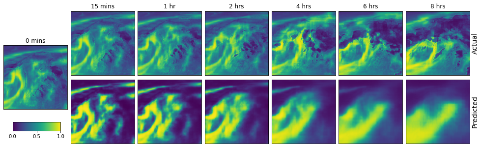
We conducted a pictorial representation and analysis of the validation data based on the effect of time. Here, the variables are plotted individually to show the trend over the time of forecasting window. The weather conditions were compared to the ground truth as shown in Figs. 4, 6, 7 and 5. This analysis shows that the model was able to accurately predict the weather variables quite well at start but its reliability decreases with time. As an example, the temperature prediction in Fig. (4) follows the expected value but slight blurriness towards the end to the prediction horizon. This is similar to the observation in the analysis of cma (fig. 5), asii_turb_trop_prob (6), and crr_intensity (7). The crr_intensity shown in figure (7) indicate that the model can learn even in scarcity of non-zero values.

5 Conclusions and Future Work

We presented for the first time a short-time weather forecasting model that uses the 3D Swin-Transformer in a UNet architecture, which resulted in competitive results, i.e., a leaderboard score (scaled multitask MSE) of 0.4750 and 0.4420, for the core and transfer challenges (IEEE Big Data Weather4Cast2021 [78]). The proposed model has only three blocks of Swin-transformers in both the encoder and decoder parts. It uses cross-attention in the decoder to merge data from the encoder with the upsampled decoding data. This ensures that the model focuses only on important information. We intend to investigate different types of attention layers in the future. Similarly, we intend to investigate token mixing using hypercomplex networks such as sedenion [21].

Acknowledgements

This work was supported by the ICT Fund, Telecommunications Regulatory Authority (TRA), Abu Dhabi, United Arab Emirates.

References

[1] X. Ren, X. Li, K. Ren, J. Song, Z. Xu, K. Deng, and X. Wang, ‘‘Deep learning-based weather prediction: A survey,’’ Big Data Research, vol. 23, p. 100178, 2021. [Online]. Available: https://www.sciencedirect.com/science/article/pii/S2214579620300460
[2] D. N. Fente and D. Kumar Singh, ‘‘Weather forecasting using artificial neural network,’’ in 2018 Second International Conference on Inventive Communication and Computational Technologies (ICICCT), 2018, pp. 1757--1761.
[3] B. Wang, J. Lu, Z. Yan, H. Luo, T. Li, Y. Zheng, and G. Zhang, ‘‘Deep uncertainty quantification: A machine learning approach for weather forecasting,’’ in Proceedings of the 25th ACM SIGKDD International Conference on Knowledge Discovery &; Data Mining, ser. KDD ’19. New York, NY, USA: Association for Computing Machinery, 2019, p. 2087–2095. [Online]. Available: https://doi.org/10.1145/3292500.3330704
[4] N. Singh, S. Chaturvedi, and S. Akhter, ‘‘Weather forecasting using machine learning algorithm,’’ in 2019 International Conference on Signal Processing and Communication (ICSC), 2019, pp. 171--174.
[5] P. Hewage, A. Behera, M. Trovati, E. Pereira, M. Ghahremani, F. Palmieri, and Y. Liu, ‘‘Temporal Convolutional Neural (TCN) Network for an Effective Weather Forecasting Using Time-Series Data from the Local Weather Station,’’ Soft Comput., vol. 24, no. 21, p. 16453–16482, nov 2020. [Online]. Available: https://doi.org/10.1007/s00500-020-04954-0
[6] P. Hewage, M. Trovati, E. Pereira, and A. Behera, ‘‘Deep Learning-Based Effective Fine-Grained Weather Forecasting Model,’’ Pattern Anal. Appl., vol. 24, no. 1, p. 343–366, feb 2021. [Online]. Available: https://doi.org/10.1007/s10044-020-00898-1
[7] M. Qiu, P. Zhao, K. Zhang, J. Huang, X. Shi, X. Wang, and W. Chu, ‘‘A Short-Term Rainfall Prediction Model Using Multi-task Convolutional Neural Networks,’’ in 2017 IEEE International Conference on Data Mining (ICDM), 2017, pp. 395--404.
[8] R. Castro, Y. M. Souto, E. Ogasawara, F. Porto, and E. Bezerra, ‘‘STConvS2S: Spatiotemporal Convolutional Sequence to Sequence Network for weather forecasting,’’ Neurocomputing, vol. 426, pp. 285--298, 2021. [Online]. Available: https://www.sciencedirect.com/science/article/pii/S0925231220315794
[9] K. Yonekura, H. Hattori, and T. Suzuki, ‘‘Short-term local weather forecast using dense weather station by deep neural network,’’ in IEEE International Conference on Big Data, Big Data. IEEE, 2018, p. 1683–1690.
[10] C.-J. Zhang, X.-J. Wang, L.-M. Ma, and X.-Q. Lu, ‘‘Tropical cyclone intensity classification and estimation using infrared satellite images with deep learning,’’ IEEE Journal of Selected Topics in Applied Earth Observations and Remote Sensing, vol. 14, pp. 2070--2086, 2021.
[11] M. Hossain, B. Rekabdar, S. Louis, and S. Dascalu, ‘‘Forecasting the weather of nevada: a deep learning approach,’’ in International Joint Conference on Neural Networks, IJCNN. IEEE, 2015, p. 1–6.
[12] S.-Y. Lin, C.-C. Chiang, J.-B. Li, Z.-S. Hung, and K.-M. Chao, ‘‘Dynamic fine-tuning stacked auto-encoder neural network for weather forecast,’’ Future Gener. Comput. Syst, vol. 89, p. 446–454, 2018.
[13] C. K. Sønderby, L. Espeholt, J. Heek, M. Dehghani, A. Oliver, T. Salimans, S. Agrawal, J. Hickey, and N. Kalchbrenner, ‘‘Metnet: A neural weather model for precipitation forecasting,’’ CoRR, vol. abs/2003.12140, 2020. [Online]. Available: https://arxiv.org/abs/2003.12140
[14] Z. Karevan and J. A. K. Suykens, ‘‘Spatio-temporal stacked lstm for temperature prediction in weather forecasting,’’ 2018.
[15] S. Hou, W. Li, T. Liu, S. Zhou, J. Guan, R. Qin, and Z. Wang, ‘‘D2cl: A dense dilated convolutional lstm model for sea surface temperature prediction,’’ IEEE Journal of Selected Topics in Applied Earth Observations and Remote Sensing, vol. 14, pp. 12 514--12 523, 2021.
[16] T. Xiong, J. He, H. Wang, X. Tang, Z. Shi, and Q. Zeng, ‘‘Contextual Sa-Attention Convolutional LSTM for Precipitation Nowcasting: A Spatiotemporal Sequence Forecasting View,’’ IEEE Journal of Selected Topics in Applied Earth Observations and Remote Sensing, vol. 14, pp. 12 479--12 491, 2021.
[17] A. Krizhevsky, I. Sutskever, and G. E. Hinton, ‘‘Imagenet classification with deep convolutional neural networks,’’ in Advances in Neural Information Processing Systems, F. Pereira, C. J. C. Burges, L. Bottou, and K. Q. Weinberger, Eds., vol. 25. Curran Associates, Inc., 2012. [Online]. Available: https://proceedings.neurips.cc/paper/2012/file/c399862d3b9d6b76c8436e924a68c45b-Paper.pdf
[18] K. He, X. Zhang, S. Ren, and J. Sun, ‘‘Deep residual learning for image recognition,’’ in 2016 IEEE Conference on Computer Vision and Pattern Recognition (CVPR), 2016, pp. 770--778.
[19] G. Huang, Z. Liu, L. Van Der Maaten, and K. Q. Weinberger, ‘‘Densely connected convolutional networks,’’ in 2017 IEEE Conference on Computer Vision and Pattern Recognition (CVPR), 2017, pp. 2261--2269.
[20] O. Ronneberger, P. Fischer, and T. Brox, ‘‘U-net: Convolutional networks for biomedical image segmentation,’’ in Medical Image Computing and Computer-Assisted Intervention -- MICCAI 2015, N. Navab, J. Hornegger, W. M. Wells, and A. F. Frangi, Eds. Cham: Springer International Publishing, 2015, pp. 234--241.
[21] A. Bojesomo, P. Liatsis, and H. Al-Marzouqi, ‘‘Traffic flow prediction using deep sedenion networks,’’ CoRR, vol. abs/2012.03874, 2020. [Online]. Available: https://arxiv.org/abs/2012.03874
[22] S. Choi, ‘‘Utilizing unet for the future traffic map prediction task traffic4cast challenge 2020,’’ CoRR, vol. abs/2012.00125, 2020. [Online]. Available: https://arxiv.org/abs/2012.00125
[23] M. Kopp, D. Kreil, M. Neun, D. Jonietz, H. Martin, P. Herruzo, A. Gruca, A. Soleymani, F. Wu, Y. Liu, J. Xu, J. Zhang, J. Santokhi, A. Bojesomo, H. A. Marzouqi, P. Liatsis, P. H. Kwok, Q. Qi, and S. Hochreiter, ‘‘Traffic4cast at neurips 2020 - yet more on the unreasonable effectiveness of gridded geo-spatial processes,’’ in Proceedings of the NeurIPS 2020 Competition and Demonstration Track, ser. Proceedings of Machine Learning Research, H. J. Escalante and K. Hofmann, Eds., vol. 133. PMLR, 06--12 Dec 2021, pp. 325--343. [Online]. Available: https://proceedings.mlr.press/v133/kopp21a.html
[24] A. Dosovitskiy, L. Beyer, A. Kolesnikov, D. Weissenborn, X. Zhai, T. Unterthiner, M. Dehghani, M. Minderer, G. Heigold, S. Gelly, J. Uszkoreit, and N. Houlsby, ‘‘An image is worth 16x16 words: Transformers for image recognition at scale,’’ ArXiv, vol. abs/2010.11929, 2021.
[25] W. Wang, E. Xie, X. Li, D.-P. Fan, K. Song, D. Liang, T. Lu, P. Luo, and L. Shao, ‘‘Pyramid vision transformer: A versatile backbone for dense prediction without convolutions,’’ ArXiv, vol. abs/2102.12122, 2021.
[26] R. Ranftl, A. Bochkovskiy, and V. Koltun, ‘‘Vision transformers for dense prediction,’’ in 2021 IEEE/CVF International Conference on Computer Vision (ICCV). Los Alamitos, CA, USA: IEEE Computer Society, oct 2021, pp. 12 159--12 168. [Online]. Available: https://doi.ieeecomputersociety.org/10.1109/ICCV48922.2021.01196
[27] Z. Dai, H. Liu, Q. V. Le, and M. Tan, ‘‘Coatnet: Marrying convolution and attention for all data sizes,’’ in Advances in Neural Information Processing Systems, M. Ranzato, A. Beygelzimer, Y. Dauphin, P. Liang, and J. W. Vaughan, Eds., vol. 34. Curran Associates, Inc., 2021, pp. 3965--3977. [Online]. Available: https://proceedings.neurips.cc/paper/2021/file/20568692db622456cc42a2e853ca21f8-Paper.pdf
[28] X. Dong, J. Bao, D. Chen, W. Zhang, N. Yu, L. Yuan, D. Chen, and B. Guo, ‘‘CSWin Transformer: A General Vision Transformer Backbone with Cross-Shaped Windows,’’ CoRR, vol. abs/2107.00652, 2021. [Online]. Available: https://arxiv.org/abs/2107.00652
[29] Z. Liu, Y. Lin, Y. Cao, H. Hu, Y. Wei, Z. Zhang, S. Lin, and B. Guo, ‘‘Swin transformer: Hierarchical vision transformer using shifted windows,’’ in 2021 IEEE/CVF International Conference on Computer Vision (ICCV), 2021, pp. 9992--10 002.
[30] Z. Liu, J. Ning, Y. Cao, Y. Wei, Z. Zhang, S. Lin, and H. Hu, ‘‘Video Swin Transformer,’’ arXiv preprint arXiv:2106.13230, pp. 1--12, 2021. [Online]. Available: http://arxiv.org/abs/2106.13230
[31] W. Wang, L. Yao, L. Chen, D. Cai, X. He, and W. Liu, ‘‘CrossFormer: A Versatile Vision Transformer Based on Cross-scale Attention,’’ CoRR, vol. abs/2108.00154, 2021. [Online]. Available: https://arxiv.org/abs/2108.00154
[32] A. Vaswani, N. Shazeer, N. Parmar, J. Uszkoreit, L. Jones, A. N. Gomez, L. u. Kaiser, and I. Polosukhin, ‘‘Attention is all you need,’’ in Advances in Neural Information Processing Systems, I. Guyon, U. V. Luxburg, S. Bengio, H. Wallach, R. Fergus, S. Vishwanathan, and R. Garnett, Eds., vol. 30. Curran Associates, Inc., 2017. [Online]. Available: https://proceedings.neurips.cc/paper/2017/file/3f5ee243547dee91fbd053c1c4a845aa-Paper.pdf
[33] H. Cao, Y. Wang, J. Chen, D. Jiang, X. Zhang, Q. Tian, and M. Wang, ‘‘Swin-Unet: Unet-like Pure Transformer for Medical Image Segmentation,’’ pp. 1--14, 2021. [Online]. Available: http://arxiv.org/abs/2105.05537
[34] A. Bojesomo, H. Al-Marzouqi, and P. Liatsis, ‘‘Spatiotemporal Vision Transformer for Short Time Weather Forecasting,’’ in 2021 IEEE International Conference on Big Data (Big Data). IEEE, 2021, pp. 5741--5746.
[35] ------, ‘‘Spatiotemporal swin-transformer network for short time weather forecasting,’’ in Proceedings of the CIKM 2021 Workshops colocated with 30th ACM International Conference on Information and Knowledge Management (CIKM 2021), Virtual Event, QLD, November 1-5, 2021, CEUR Workshop Proceedings. Association for Computing Machinery, 2021.
[36] A. Bojesomo, H. Al-Marzouqi, and P. Liatsis, ‘‘SwinUNet3D - A Hierarchical Architecture for Deep Traffic Prediction using Shifted Window Transformers,’’ CoRR, vol. abs/2201.06390, 2022. [Online]. Available: https://arxiv.org/abs/2201.06390
[37] R. Goyal, S. Ebrahimi Kahou, V. Michalski, J. Materzynska, S. Westphal, H. Kim, V. Haenel, I. Fruend, P. Yianilos, M. Mueller-Freitag et al., ‘‘The" something something" video database for learning and evaluating visual common sense,’’ in Proceedings of the IEEE international conference on computer vision, 2017, pp. 5842--5850.
[38] W. Kay, J. Carreira, K. Simonyan, B. Zhang, C. Hillier, S. Vijayanarasimhan, F. Viola, T. Green, T. Back, P. Natsev et al., ‘‘The kinetics human action video dataset,’’ arXiv preprint arXiv:1705.06950, 2017.
[39] P. Bauer, A. Thorpe, and G. Brunet, ‘‘The quiet revolution of numerical weather prediction,’’ Nature, vol. 525, p. 47–55, 2015.
[40] I. Sandu, A. Beljaars, P. Bechtold, T. Mauritsen, and G. Balsamo, ‘‘Why is it so difficult to represent stably stratified conditions in numerical weather prediction (nwp) models?’’ Journal of Advances in Modeling Earth Systems, vol. 5, no. 2, pp. 117--133, 2013.
[41] A. Abraham, N. Philip, B. Nath, and P. Saratchandran, ‘‘Performance analysis of connectionist paradigms for modeling chaotic behavior of stock indices,’’ in Second International Workshop on Intelligent Systems Design and Applications, Computational Intelligence and Applications. USA: Dynamic Publishers Inc, 2002, p. 181–186.
[42] C. Voyant, M. Muselli, C. Paoli, and M.-L. Nivet, ‘‘Numerical weather prediction (nwp) and hybrid arma/ann model to predict global radiation,’’ Energy, vol. 39, no. 1, pp. 341--355, 2012.
[43] J. Pathak, B. Hunt, M. Girvan, Z. Lu, and E. Ott, ‘‘Model-free prediction of large spatiotemporally chaotic systems from data: A reservoir computing approach,’’ Physical review letters, vol. 120, no. 2, p. 024102, 2018.
[44] C. He, J. Wei, Y. Song, and J.-J. Luo, ‘‘Seasonal prediction of summer precipitation in the middle and lower reaches of the yangtze river valley: Comparison of machine learning and climate model predictions,’’ vol. 13, no. 22, 2021. [Online]. Available: https://www.scopus.com/inward/record.uri?eid=2-s2.0-85119970664&doi=10.3390%2fw13223294&partnerID=40&md5=5f871022a5647c9c95094d77049655f3
[45] B. Bochenek and Z. Ustrnul, ‘‘Machine learning in weather prediction and climate analyses—applications and perspectives,’’ vol. 13, no. 2, 2022. [Online]. Available: https://www.scopus.com/inward/record.uri?eid=2-s2.0-85124086690&doi=10.3390%2fatmos13020180&partnerID=40&md5=af5d57af5589fe9a98d64c7dd8291c2d
[46] E. Juarez and M. Petersen, ‘‘A comparison of machine learning methods to forecast tropospheric ozone levels in delhi,’’ vol. 13, no. 1, 2022. [Online]. Available: https://www.scopus.com/inward/record.uri?eid=2-s2.0-85121997176&doi=10.3390%2fatmos13010046&partnerID=40&md5=63c12de7bb39846e3af8a01b6db25747
[47] M. Achite, M. Jehanzaib, N. Elshaboury, and T.-W. Kim, ‘‘Evaluation of machine learning techniques for hydrological drought modeling: A case study of the wadi ouahrane basin in algeria,’’ vol. 14, no. 3, 2022. [Online]. Available: https://www.scopus.com/inward/record.uri?eid=2-s2.0-85123691238&doi=10.3390%2fw14030431&partnerID=40&md5=afcb2f30df6d19e09caf83f671dcd268
[48] Y. Fang, H. Chen, Y. Lin, C. Zhao, Y. Lin, and F. Zhou, ‘‘Classification of northeast china cold vortex activity paths in early summer based on k-means clustering and their climate impact,’’ Advances in Atmospheric Sciences, vol. 38, no. 3, pp. 400--412, 2021.
[49] D. Lou, M. Yang, D. Shi, G. Wang, W. Ullah, Y. Chai, and Y. Chen, ‘‘K-means and c4.5 decision tree based prediction of long-term precipitation variability in the poyang lake basin, china,’’ vol. 12, no. 7, 2021. [Online]. Available: https://www.scopus.com/inward/record.uri?eid=2-s2.0-85109636880&doi=10.3390%2fatmos12070834&partnerID=40&md5=721615d85cc65ee47a06e944513f19c7
[50] J. Abbot and J. Marohasy, ‘‘The application of machine learning for evaluating anthropogenic versus natural climate change,’’ GeoResJ, vol. 14, pp. 36--46, 2017.
[51] W. Almikaeel, L. Čubanová, and A. Šoltész, ‘‘Hydrological drought forecasting using machine learning—gidra river case study,’’ vol. 14, no. 3, 2022. [Online]. Available: https://www.scopus.com/inward/record.uri?eid=2-s2.0-85123703263&doi=10.3390%2fw14030387&partnerID=40&md5=44b26539167a4ecc0ebc381cd2fc6563
[52] M. Ma, P. Xie, F. Teng, T. Li, B. Wang, S. Ji, and J. Zhang, ‘‘Histgnn: Hierarchical spatio-temporal graph neural networks for weather forecasting,’’ arXiv preprint arXiv:2201.09101, 2022.
[53] B. P. Shukla, C. M. Kishtawal, and P. K. Pal, ‘‘Prediction of satellite image sequence for weather nowcasting using cluster-based spatiotemporal regression,’’ IEEE transactions on geoscience and remote sensing, vol. 52, no. 7, pp. 4155--4160, 2013.
[54] ‘‘Day-ahead spatiotemporal solar irradiation forecasting using frequency-based hybrid principal component analysis and neural network,’’ Applied Energy, vol. 247, pp. 389--402, 2019. [Online]. Available: https://www.sciencedirect.com/science/article/pii/S0306261919307019
[55] L. Huang, J. Kang, M. Wan, L. Fang, C. Zhang, and Z. Zeng, ‘‘Solar radiation prediction using different machine learning algorithms and implications for extreme climate events,’’ Frontiers in Earth Science, vol. 9, p. 202, 2021.
[56] D. Niu, L. Diao, Z. Zang, H. Che, T. Zhang, and X. Chen, ‘‘A machine-learning approach combining wavelet packet denoising with catboost for weather forecasting,’’ vol. 12, no. 12, 2021. [Online]. Available: https://www.scopus.com/inward/record.uri?eid=2-s2.0-85122790317&doi=10.3390%2fatmos12121618&partnerID=40&md5=c382761cb7f88374815f99aa1f604af0
[57] V. Monego, J. Anochi, and H. de Campos Velho, ‘‘South america seasonal precipitation prediction by gradient-boosting machine-learning approach,’’ vol. 13, no. 2, 2022. [Online]. Available: https://www.scopus.com/inward/record.uri?eid=2-s2.0-85124129167&doi=10.3390%2fatmos13020243&partnerID=40&md5=bebfbce74f66e6d71dae103a9f348181
[58] L. Iverson, A. Prasad, and A. Liaw, ‘‘New machine learning tools for predictive vegetation mapping after climate change: Bagging and random forest perform better than regression tree analysis,’’ in In: Smithers, Richard, ed. Landscape ecology of trees and forests, proceedings of the twelfth annual IALE (UK) conference; 2004 June 21-24; Cirencester, UK.[Place of publication unknown]: International Association for Landscape Ecology: 317-320., 2004.
[59] P.-S. Yu, T.-C. Yang, S.-Y. Chen, C.-M. Kuo, and H.-W. Tseng, ‘‘Comparison of random forests and support vector machine for real-time radar-derived rainfall forecasting,’’ vol. 552, pp. 92--104, 2017. [Online]. Available: https://www.scopus.com/inward/record.uri?eid=2-s2.0-85021687551&doi=10.1016%2fj.jhydrol.2017.06.020&partnerID=40&md5=a15fba257a86853e0788f5fa78c16555
[60] C. Song, X. Chen, P. Wu, and H. Jin, ‘‘Combining time varying filtering based empirical mode decomposition and machine learning to predict precipitation from nonlinear series,’’ vol. 603, 2021. [Online]. Available: https://www.scopus.com/inward/record.uri?eid=2-s2.0-85116582095&doi=10.1016%2fj.jhydrol.2021.126914&partnerID=40&md5=9d1640a89522d66d5298b824804ed5c8
[61] J. N. Liu, Y. Hu, J. J. You, and P. W. Chan, ‘‘Deep neural network based feature representation for weather forecasting,’’ in Proceedings on the International Conference on Artificial Intelligence (ICAI). The Steering Committee of The World Congress in Computer Science, Computer …, 2014, p. 1.
[62] S.-Y. Lin, C.-C. Chiang, J.-B. Li, Z.-S. Hung, and K.-M. Chao, ‘‘Dynamic fine-tuning stacked auto-encoder neural network for weather forecast,’’ Future Generation Computer Systems, vol. 89, pp. 446--454, 2018. [Online]. Available: https://www.sciencedirect.com/science/article/pii/S0167739X17329801
[63] J. Leinonen, ‘‘Improvements to short-term weather prediction with recurrent-convolutional networks,’’ CoRR, vol. abs/2111.06240, 2021. [Online]. Available: https://arxiv.org/abs/2111.06240
[64] S. Choi, ‘‘UNet based future weather prediction on Weather4cast 2021 stage 2,’’ in 2021 IEEE International Conference on Big Data (Big Data), 2021, pp. 5747--5749.
[65] P. H. Kwok and Q. Qi, ‘‘Enhanced variational u-net for weather forecasting,’’ in 2021 IEEE International Conference on Big Data (Big Data), 2021, pp. 5758--5763.
[66] S. Ravuri, K. Lenc, M. Willson, D. Kangin, R. Lam, P. Mirowski, M. Fitzsimons, M. Athanassiadou, S. Kashem, S. Madge et al., ‘‘Skilful precipitation nowcasting using deep generative models of radar,’’ Nature, vol. 597, no. 7878, pp. 672--677, 2021.
[67] C. Wang, P. Wang, P. Wang, B. Xue, and D. Wang, ‘‘Using conditional generative adversarial 3-d convolutional neural network for precise radar extrapolation,’’ IEEE Journal of Selected Topics in Applied Earth Observations and Remote Sensing, vol. 14, pp. 5735--5749, 2021.
[68] X. Shi, Z. Chen, H. Wang, D.-Y. Yeung, W.-k. Wong, and W.-c. Woo, ‘‘Convolutional lstm network: A machine learning approach for precipitation nowcasting,’’ in Proceedings of the 28th International Conference on Neural Information Processing Systems - Volume 1, ser. NIPS’15. Cambridge, MA, USA: MIT Press, 2015, p. 802–810.
[69] Y. Wang, M. Long, J. Wang, Z. Gao, and P. S. Yu, ‘‘Predrnn: Recurrent neural networks for predictive learning using spatiotemporal lstms,’’ in Advances in Neural Information Processing Systems, I. Guyon, U. V. Luxburg, S. Bengio, H. Wallach, R. Fergus, S. Vishwanathan, and R. Garnett, Eds., vol. 30. Curran Associates, Inc., 2017. [Online]. Available: https://proceedings.neurips.cc/paper/2017/file/e5f6ad6ce374177eef023bf5d0c018b6-Paper.pdf
[70] Y. Wang, Z. Gao, M. Long, J. Wang, and P. S. Yu, ‘‘PredRNN++: Towards a resolution of the deep-in-time dilemma in spatiotemporal predictive learning,’’ in Proceedings of the 35th International Conference on Machine Learning, ser. Proceedings of Machine Learning Research, J. Dy and A. Krause, Eds., vol. 80. PMLR, 10--15 Jul 2018, pp. 5123--5132. [Online]. Available: https://proceedings.mlr.press/v80/wang18b.html
[71] X. Shi, Z. Gao, L. Lausen, H. Wang, D.-Y. Yeung, W.-k. Wong, and W.-c. Woo, ‘‘Deep learning for precipitation nowcasting: A benchmark and a new model,’’ ser. NIPS’17. Red Hook, NY, USA: Curran Associates Inc., 2017, p. 5622–5632.
[72] S. Huang, Z. Lu, R. Cheng, and C. He, ‘‘FaPN: Feature-aligned pyramid network for dense image prediction,’’ in International Conference on Computer Vision (ICCV), 2021.
[73] T. Xiao, Y. Liu, B. Zhou, Y. Jiang, and J. Sun, ‘‘Unified perceptual parsing for scene understanding,’’ in European Conference on Computer Vision. Springer, 2018.
[74] E. Xie, W. Wang, Z. Yu, A. Anandkumar, J. M. Alvarez, and P. Luo, ‘‘Segformer: Simple and efficient design for semantic segmentation with transformers,’’ in Advances in Neural Information Processing Systems, A. Beygelzimer, Y. Dauphin, P. Liang, and J. W. Vaughan, Eds., 2021. [Online]. Available: https://openreview.net/forum?id=OG18MI5TRL
[75] L. J. Ba, J. R. Kiros, and G. E. Hinton, ‘‘Layer normalization,’’ CoRR, vol. abs/1607.06450, 2016. [Online]. Available: http://arxiv.org/abs/1607.06450
[76] A. Chaurasia and E. Culurciello, ‘‘LinkNet: Exploiting encoder representations for efficient semantic segmentation,’’ 2017 IEEE Visual Communications and Image Processing (VCIP), Dec 2017. [Online]. Available: http://dx.doi.org/10.1109/VCIP.2017.8305148
[77] A. Gruca, P. Herruzo, P. Rípodas, A. Kucik, C. Briese, M. K. Kopp, S. Hochreiter, P. Ghamisi, and D. P. Kreil, ‘‘Cdceo’21 - first workshop on complex data challenges in earth observation,’’ in Proceedings of the 30th ACM International Conference on Information & Knowledge Management, ser. CIKM ’21. New York, NY, USA: Association for Computing Machinery, 2021, p. 4878–4879. [Online]. Available: https://doi.org/10.1145/3459637.3482044
[78] ‘‘Multi-sensor weather forecast competition : IEEE Big Data Cup 2021 Leaderboard,’’ https://www.iarai.ac.at/weather4cast/competitions/ieee-big-data-core-final/?leaderboard, 2021.
[79] D. P. Kingma and J. Ba, ‘‘Adam: A method for stochastic optimization,’’ CoRR, vol. abs/1412.6980, 2015.
[80] I. Rangwala and J. R. Miller, ‘‘Climate change in mountains: a review of elevation-dependent warming and its possible causes,’’ Climatic change, vol. 114, no. 3, pp. 527--547, 2012.
[81] M. Kuhn and M. Olefs, ‘‘Elevation-dependent climate change in the european alps,’’ 12 2020. [Online]. Available: https://oxfordre.com/climatescience/view/10.1093/acrefore/9780190228620.001.0001/acrefore-9780190228620-e-762