A Novel Rapid-flooding Approach with Real-time Delay Compensation for Wireless Sensor Network Time Synchronization
Abstract
One-way-broadcast based flooding time synchronization algorithms are commonly used in wireless sensor networks (WSNs). However, the packet delay and clock drift pose challenges to accuracy, as they entail serious by-hop error accumulation problems in the WSNs. To overcome it, a rapid-flooding multi-broadcast time synchronization with real-time delay compensation (RDC-RMTS) is proposed in this paper. By using a rapid-flooding protocol, flooding latency of the referenced time information is significantly reduced in the RDC-RMTS. In addition, a new joint clock skew-offset maximum likelihood estimation is developed to obtain the accurate clock parameter estimations, and the real-time packet delay estimation. Moreover, an innovative implementation of the RDC-RMTS is designed with an adaptive clock offset estimation. The experimental results indicate that, the RDC-RMTS can easily reduce the variable delay and significantly slow the growth of by-hop error accumulation. Thus, the proposed RDC-RMTS can achieve accurate time synchronization in large-scale complex WSNs.
Index Terms:
Wireless Sensor Networks, Time Synchronization, Rapid Flooding, Real-time Delay Estimation, Networked and Distributed Control, Wireless Control SystemsI Introduction
Synchronization is the typical problem in distributed system, and it still remains a popular topic in smart grid [PDU_Grid], Internet of Things (IoT) [IoT1, IoT2], wireless sensor networks (WSNs) [WSN], networked synchronization control [DisControl2, DisControl4], and so on. Specifically, the time synchronization, which aims to correct the local time information on the distributed nodes and drive a common time notion network-wide, is an essential portion of some WSN/IoT applications, e.g., providing accurate time interval for distributed data acquisition and processing [DataSync, Sleep1], and scheduling [Scheduling]; measuring time delay in industrial wireless feedback control system [SyncCtrl]. However, the large-scale wireless network application imposes exceedingly strict requirements on time synchronization, for instance, they require an accuracy of about µs and µs in the industrial automation standards ISA100.11a [ISA-100.11a] and WirelessHART [WirelessHART], respectively; about 120 µs for the damage localization in the structural health monitoring [SHM_erro, SHM_S]. Considering WSN is being used in many applications, e.g., industrial automation, monitoring, and is resource-constrained, low-cost, large scale and unreliable connection, therefore its time synchronization problem is representative.
The early researches focused on developing novel synchronization structures, reducing the dependence of the algorithms on the network topology management, and improving the robustness of the algorithms in dynamic networks. As is known to all, due to the requirement of additional protocol to manage the topology of network, the RBS [RBS] and the TPSN [TPSN] are difficult to be deployed in a large-scale complex network, which has large diameter and dynamic topology. Many of the derived algorithms were expected to optimize the implementation complexity, e.g., the clustered-based algorithm [cluster-Conse-sync-1, PulseSS, cluster-Conse-sync-2, cluster-Conse-sync-3] and low-power interested approach in [CESP], the improved two-way message exchange time synchronization approaches in [TSync, Timing-sync, Star-Structure, Elsharief2017DensityTable, R-Sync, Q_TTME, TT_K, TT_W].
In recent years, the flooding time synchronization algorithms [FTSP, FCSA, PulseSync, RMTS] and the consensus-based approaches [ATS2007A, ATS, DCTS, GTSP] are widely studied to meet the accurate synchronization in the large-scale complex WSN. These time synchronization algorithms do not require any topology management, so the problems mentioned above are naturally avoided. Moreover, they are robust and scalable, and can adapt quickly to the changes in network connectivity and clock drifts. However, there are limitations to both of the flooding and the consensus-based methods. In other words, they are different from each other and can be used to meet the time synchronization requirements in different WSNs.
Considering a consensus-based time synchronization algorithm, it is easy to implement and robust in dynamic networks. However, its convergence rate is very slow due to the iteration. For instance, the convergence time is up to 120 rounds of synchronization intervals in ATS ( grid network) [ATS], and studies in [CCS, EventDriven_ATS, MTS, DiStiNCT, HE2017C, MACTS] are interested in improving the convergence rate. However, It cannot to be synchronized by an external clock or the heterogeneous network [EGsync]. What it matters is not the value of the reference clock but the fact that all clocks converge to one common virtual reference, thus it cannot be synchronized with an external clock or the heterogeneous network [EGsync].
Fortunately, flooding time synchronization algorithm can easily avoid the problems in a consensus-based method. It employs a special node as the reference, meanwhile it distributes the reference’s time information network-wide and aims to synchronize all of the nodes to the reference. A number of line networks are automatically generated while the referenced time information is flooded. Therefore, a complex network is simplified as lines, and the distance of line is the main factor of network to affect the algorithm. The rapid-flooding protocol leads the algorithms to build a stable synchronization after a few synchronization intervals, e.g., about 3 rounds in RMTS ( grid network) [RMTS]. Moreover, the rapid-flooding is a synchronous method in which the time interval of node transmission can be predicted, thus it is possible and easy to meet synchronous sleep/wake scheduling for low-duty cycle WSN [Chase, Splash]. Hence, the flooding time synchronization algorithm will be a very efficient solution for the time synchronization in the large-scale WSNs.
However, distance of flooding path, flooding latency, packet delay, and clock drift, which cause the unpredictable by-hop error accumulation problem, pose the main challenges to a flooding time synchronization algorithm. Such problems have been significantly improved by the previous studies, and most of the recent studies on flooding time synchronization focus on improving the accuracy, e.g., PulseSync [PulseSync_1, PulseSync], Glossy [glossy], FCSA [FCSA], RMTS [RMTS]. The improvements of flooding time synchronization are simple and effective, i.e., shortening the flooding latency and removing the delay, meanwhile compensating the clock drift. However, there is no better way to calculate packet delay in existing one-way broadcast-based synchronization protocols, but using the prior constant, e.g., the method used in PulseSync and RMTS. Hence, before deploying WSN, a lot of preliminary experiments are required to calculate the prior constant; actual delay may change due to hardware and environment changes.
In this paper, we are interested in a real-time and agile delay estimation to improve the rapid-flooding time synchronization. If the clock skew estimation is fast convergence and independent of the clock offset estimation, meanwhile if a two-way message exchange can be constructed in the one-way-broadcast model, then the real-time delay compensation can be implemented. It is worth mentioning that this strategy has been inspired by the two-way message exchange model based clock offset estimation in [DRJeskeMLE, KLNohMLE, QMChaudhariMLE]. To achieve the objective, the Maximum Likelihood Estimation (MLE) proposed in [MLE] is employed to generate an accurate clock skew estimation at the second round of synchronization; meanwhile an improved two-way message exchange model is constructed on one-way-broadcast model; then a joint clock skew-offset MLE is obtained , and the real-time delay estimation is also given. As a result, a new rapid-flooding multi-broadcast time synchronization with real-time delay compensation (RDC-RMTS) protocol is further developed. The main contributions of this work are as follows.
1) A novel two-way message exchange model is ingeniously designed in the one-way broadcast-based flooding time synchronization, which utilizes redundant broadcasting without any additional packet transmission.
2) The proposed joint clock skew-offset MLE provides the real-time delay estimations and the accurate clock offset estimation, which results in better scalability to RDC-RMTS.
3) An innovate implementation is developed for the RDC-RMTS, in which an adaptive clock offset estimation is designed to guarantee the accurate estimation over unreliable network.
Moreover, the actual performances of flooding time synchronization in a large-scale complex network are discussed. Basically, the performance evaluation indicate that the network mainly affect the time synchronization in a way of increasing the flooding path.
The rest of the paper is organized as follows. In Section II, the challenges to the flooding time synchronization is discussed in detail, and the motivation of this paper is provided. The system model is provided in Section III and the RDC-RMTS is proposed in Section IV. The implementation of RDC-RMTS is described in Section V. The RDC-RMTS is evaluated and discussed in Section VI, where the testbed is provided, and the experimental results in FTSP, FCSA, FloodPISync, PulseSync, PulsePISync, and RMTS are also reported. The discussions and simulations results in complex network are reported in Section VII. Finally, conclusions are drawn in Section VIII.
II Challenges and Motivation
Flooding time synchronization protocol is easy to implement, and does not require topology management. In addition, flooding operations decompose a complex network into multi-line networks, then the nodes on the line synchronize itself to the reference node (root). However, the time synchronization on a multi-hop node depends on the time information forwarded by relay nodes, thus relay node synchronization error will accumulate on a hop-by-hop basis, i.e., by-hop error accumulation problem [RMTS], which is the major challenge to flooding time synchronization.
A by-hop error accumulation is mainly caused by flooding latency, packet transmission delay, and clock drift. In addition, it is proportional to the distance of reference node and multi-hop node. Definition is the synchronization error of the node relative to the reference node, then the synchronization error on the -hop node which is derived in [RMTS], is given by
| (1) |
where , which is less than the synchronization interval (), is the flooding latency at the -hop node, and is the relative clock rate between -hop and ()-hop.Variable is one-way broadcast packet transmission delay at the hop node, which comprises variable portion and uncertain portion [RMTS]. Moreover, , where constant is the mean of , and variable ( is the standard deviation of ). Hence, . Because relative clock rate or clock frequency offset is usually described in parts per million (PPM), a multiplier is used in (1).
Summaries of the existing flooding time synchronization algorithms are shown in Table I. It should be noted that, according to the [FCSA, PISync], although they don’t seems emphasize the use of to compensate clock offset estimation, we prefer to do this in our experiments to get better experimental results. Moreover, is calculated during the experimental phase based on the previous experimental results, and it is a constant when the algorithm is evaluated.
Summary of the flooding time synchronization algorithms in comparison. Considering the pairwise timestamps (created at sender) and (created at receiver), clock offset estimations , , and .
| Protocol | Clock Parameter Estimations | ||
|---|---|---|---|
| Clock Offset | Clock Skew | ||
| FTSP | Slow-flooding | LR | |
| FCSA | Slow-flooding | LR | |
| FloodPISync | Slow-flooding | PI | |
| PulseSync | Rapid-flooding | LR | |
| PulsePISync | Rapid-flooding | PI | |
| RMTS | Rapid-flooding | MLE | |
Lenzen et al. pointed out that, when the referenced time information is flooded network-wide, it will lose accuracy due to clock drift and flooding latency [PulseSync_1]. The PulseSync suggests to distribute time information as fast as possible, and is expected to adapt to fast change in clock drift. Unlike FTSP, which uses slow-flooding, PulseSync uses a rapid-flooding protocol. The Glossy and RMTS are also rapid-flooding approaches.
The FCSA tries to minimize the undesired effect of flood waiting times on the synchronization accuracy by using a clock rate agreement algorithm, and expects to force all nodes to agree on a common clock rate. Even so, the slight estimation error on clock skew estimation may cause serious interference to time synchronization accuracy. Especially, the FCSA use linear regression (LR) to estimate the clock skew, where the is directly introduced in observations. By using LR, the problem in FCSA also exists in FTSP and PulseSync. The PISync employs a Proportion Integration (PI) control method to optimize the clock skew estimation, however the delays in the observations are not optimized. Unlike that, the MLE in [MLE, RMTS] tries to minimize the delay and could obtain more accurate clock skew estimation than LR and PI method [MLE].
The existing flooding time synchronization algorithms use accurate clock parameter estimation methods and rapid-flooding protocol, and are expected to against the by-hop error accumulation problem. Considering the by-hop error accumulation model in (1), the FCSA tries to minimize , moreover, the PulseSync and RMTS are also to minimize . As discussed in [RMTS], the summary of the synchronization error in flooding time synchronization algorithms is shown in II. It is clear that, the accuracy is significantly improved in the existing flooding time synchronization algorithms.
Summary of the synchronization error in flooding time synchronization algorithms, where . The synchronization error in FloodPISync and PulsePISync are similar to FCSA and PulseSync, respectively.
| Synchronization Error | ||
|---|---|---|
| Single-hop | -hop | |
| FTSP | (1) | |
| FCSA | ||
| PulseSync | ||
| RMTS | ||
PulseSync and RMTS use a fixed delay estimation for clock offset estimate compensation that pose challenges to flexible deployment, as it entails that a lot of preliminary experiments need to be completed for the delay estimation. Testbed is needed to collect experimental results and calculate delay estimation, and the estimation cannot be changed after being deployed. Thus, the synchronization accuracy of algorithm may decrease results from the timely changes in delay.
In the light of the above discussion, the main motivation of this paper is to obtain a timely delay estimation, and then propose a new rapid-flooding time synchronization algorithm with real-time delay compensation against the by-hop error accumulation problem.
III System Model
The WSN is modeled as the graph , where represents the nodes of the WSN and defines the available communications links. The set of neighbors for is , where nodes and belong to , and . In our work, there are two time notions defined for the time synchronization algorithm, i.e. the hardware clock notion and logical clock notion . Hardware clock is defined as
| (2) |
where is the hardware clock notion. Parameter is the hardware frequency rate (clock speed) of the clock source, meanwhile it is the inherent attribute of crystal oscillator and cannot be changed or measured. Any node considers itself to have the ideal clock frequency (i.e. nominal frequency) and . Variable is the moment that node is powered on, and is the initial relative clock offset. It should be noticed that cannot be changed either, and the timestamps on are used to estimate the relative clock speed for the proposed algorithm.
The logical clock is defined as
| (3) |
where is the logical relative clock rate and initialized as 1, it can be changed to speed up or slow down . With respect to the reference node, is always set as 1. The timestamps on are used to estimate the relative clock offset for the proposed algorithm. Variable is used to supply the global time service for the synchronization applications.
Considering the arbitrary nodes and , and are the logical times respectively, and is the relative logical frequency rate which is
| (4) |
where, in consideration of arbitrary moments and , . The relative clock offset increment in is . Parameter is the changing rate on the relative clock offset in . It is common estimated by any two clock offset estimations and used to compensate the clock skew in the time synchronization algorithms.
IV Proposed RDC-RMTS Algorithm
Considering the one-way broadcast based time synchronization protocols, and assuming that the clock skew is fixed in a short time, the key idea of RDC-RMTS is that: the clock skew estimation is independent of clock offset estimation, and convergence fast and accurate, then; an improved two-way message exchange can be structured for the clock offset estimation based on the one-way broadcasts, and the delay can be estimated and compensated timely in the RDC-RMTS.
IV-A Proposed Synchronization Model of RDC-RMTS
In this part, an rapid-flooding synchronization model is proposed for the RDC-RMTS based on multiple one-way broadcast, which is illustrated in Fig. 1. There are two important portions in the proposed model, i.e. multi-broadcast clock skew estimation and two-way message exchange clock offset estimation. The main difference between the new proposed synchronization model and the previous ones is that a novel two-way message exchange model is structured in the one-way broadcast synchronization model.
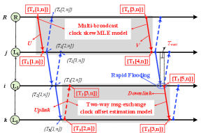
Considering the arbitrary periodically broadcasts a group of synchronization packets to neighboring nodes over a broadcast period of . Here we define as the set of timestamps at node , its size is , and is its serial number. There are packets broadcasted in a short time, and pairs of timestamps are generated. When a node broadcasts a packets, the timestamp will be created at both of the sender and the receivers.
Clock skew MLE of the RDC-RMTS is developed based on the multi-broadcast clock skew estimation, and uses two groups of multi-broadcast process (e.g., and ) to collect observations, e.g. and . Clock offset estimation of RDC-RMTS is developed based on the two-way message exchange model and the above clock skew estimation, e.g. and . Since that the time interval from the first broadcast to latest broadcast (e.g., , when , which is less than 12 microsecond in our experiments) is exceedingly short, we can assume that the relative clock offset is fixed at the phase of a multi-broadcast processing.
The RDC-RMTS is a rapid flooding time synchronization approach: the reference node initializes an synchronization period and nodes forward the newly time information to its neighbors quickly (the message flooding latency is very short).
IV-B The Clock Skew Estimation
Assuming the actual delay is Gaussian distribution, the clock skew MLE is proposed in [MLE].
In this paper, the proposed synchronization model in Fig. 1 provides an reasonable implementation for the MLE, i.e. the multi-broadcast clock skew estimation model (synchronization process and ). A group of timestamp observations is created in the multi-broadcast process, i.e., and , then the observations for the clock skew MLE likelihood function are
| (5) |
where , .
Accordingly, the clock skew MLE is
| (6) |
where is the time interval of and , e.g., .
It is worth mentioning that the is independent of clock offset estimation, and the timestamps for is generated at the hardware clock timer.
IV-C Proposed Joint Clock Skew-offset MLE
According to [TPSN], the clock offset estimation based on two-way message exchange model significantly optimizes the estimation error caused by delay, and more accurate than that of one-way broadcast model. Most of the previous clock offset MLEs, e.g., [DRJeskeMLE, KLNohMLE, QMChaudhariMLE], are developed based on two-way message exchange model. However, the traditional two-way message exchange model is implemented on a pair of nodes, thus the reference should synchronize the neighbors one by one, and it may fail to meet the efficient time synchronization over a large-scale network due to the pairwise message exchange and hierarchical management.
In this part, we employ the MLE clock skew to calculate the clock offset estimation, which is significantly different from the traditional method, e.g. the FTSP in which the linear regression is used to calculate clock skew estimations. It is worthy to note that, the MLE clock skew is independent of the clock offset estimation, therefore it is possible to use the accurate clock skew estimation to compensate the clock offset estimation.
According to the two-way message exchange clock offset estimation model that is shown in Fig. 1, for and , the timestamps are , and the timestamps are . We define that and as
| (7) |
| (8) |
where is the relative clock offset in , and , then the two-way message exchange clock offset estimation can be rewritten as
| (9) |
| (10) |
Considering that is variable value with fixed portion and variable portion , and using the (i.e., , the clock offset estimation MLE of clock offset is
| (11) |
According to [DRJeskeMLE], the MLE of joint clock skew-offset estimation is
| (12) |
where the is removed from the clock offset estimation. The is given by
| (13) |
It is worth mentioning that the timestamps for are generated at the logical clock timer.
IV-D Min function-based MLE
According to [RMTS], it is because in the observations and is always a positive value , i.e., , the min function-based MLE tries to find out the observation with minimal value of . For instance, the given by
| (14) |
where is the delay estimation, which can be calculated by (13).
IV-E Error Analysis
According to (12) and (14), the and could be removed from the error link of the RDC-RMTS. Then the single-hop synchronization error of RDC-RMTS is given by
| (15) |
By using the rapid-flood protocol and accurate clock skew compensation, the part in (1) is almost equal to 0 (), thus the by-hop error accumulation in RDC-RMTS is given by
| (16) |
which is the same as that in RMTS [RMTS].
V Implementation
The proposed RDC-RMTS removes the from clock offset estimation based on the improved two-way message exchange model without any prior knowledge. It is well known that the two-way message exchange model based synchronization algorithms (e.g. TPSN) calculate the clock offset estimation and delay separately. In this part, we demonstrate an innovative implementation for the two-way message exchange based joint clock skew-offset MLE proposed in (12) and (14).
V-A The Structure Overview of RDC-RMTS
According to (6), it suggests larger observation interval to obtain the more accurate clock skew estimation . Thus a sliding window is employed in RDC-RMTS, where is several times the actual synchronization period .
Figure 2 indicates the structure of implementation in RDC-RMTS. Considering and its neighbor , it is mainly composed of three parts: sliding window, clock skew estimation, and clock offset estimation.
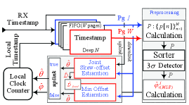
A -pages () timestamp FIFO (first in first out) buffer is the key to the sliding window. It is designed to buffer multiple groups of timestamp, and the sliding window with specified width will be generated for by copying the timestamp of the corresponding position of the FIFO. The pages () of FIFO should be larger than the maximal width of sliding window. The depth of the page is the same as the multiple number . If the sliding window length is set to be , then the is calculated based on the latest timestamp observations (Pg ) and the -th from last (i.e.,Pg ), and the in (6) is times of the synchronization period , i.e., .
1) The clock skew estimation
As discussed above, the is inevitable in the one-way broadcast. Moreover, it is not Gaussian distribution and much larger than the (which is Gaussian variable). Thus, the observations need to be preprocessed to meet the assumption (the delay is Gaussian distribution) for in (6). The is implemented in three steps: the observation calculation in (5), outlier detector (Sort and detector), and calculation in (6). Since the has extremely low probability, one can assume that the possible samples will be moved to the end of by the Sort. The can be calculated from the front observations, e.g., std. Then the possible observations will be recognized and removed from by outlier detector.
2) The adaptive clock offset estimation
Considering the large-scale complex WSN, the wireless channel collision probability will increase at in the rapid-flooding. The rapid-flooding protocol requires the higher level nodes to forward the received time information immediately, then it will be a high probability that the adjacent nodes broadcast packets at the same moment. In other words, the low level nodes can not receive all of the messages, and it will cause the in (12) to be unachievable.
To solve this issue, an adaptive approach is developed based on double clock offset estimations, i.e., the joint clock skew-offset MLE, and the min function-based MLE.
Case true: the RDC-RMTS employs the joint clock skew-offset MLE. The of two-way message exchange model is the latest multi-broadcast process of , and the is the latest multi-broadcast process of , and . parameter is calculated by (12), and the is calculated by (13).
Case false: the RDC-RMTS employs the min function-based MLE. The observations of are used, and is calculated by (14), is the average of the valid value calculated by (13). The of two-way message exchange model is the latest multi-broadcast process of .
Therefore, when the works, the is calculated. The RDC-RMTS does not requires any prior experiments to set a fixed just like RMTS, but uses a timely delay compensation. Moreover, the receiver calculates separately for different nodes. Thus, the slight differences on delay caused by the hardware differences of nodes will be handled in RDC-RMTS, while they are directly ignored in PulseSync and RMTS.
V-B The Implementation of RDC-RMTS
In this Section, we discuss the implementation of the proposed RDC-RMTS algorithm in details. For ease of description, considering the pair of adjacent nodes in Fig. 1, the node that has the lower level is defined as father, and the higher one as son, e.g. is the father of , and is the father of . In addition, the sliding window length is set as 2.
The RDC-RMTS can use the specified node as the root (reference) in WSN applications, e.g., the sink node, or the gateway node (the interface of heterogeneous networks). The flooding time synchronization cannot maintain the network-wide synchronization without an active root. Hence the RDC-RMTS employs a simple root election protocol which is used in [FTSP, FCSA, RMTS] to find a new root when the current root is invalid.
According to the synchronization model (Fig. 1) and the implementation structure (Fig. 2) of RDC-RMTS, a root (reference) algorithm and non-root algorithm are designed for the RDC-RMTS protocol.
1) The root algorithm: The periodic synchronization is created at root, and the reference’s time information is embedded into the multi-broadcast packets and flooded in the network. Meanwhile, the root will listen for broadcast messages from neighbors and store the timestamps for the joint clock skew-offset estimation.
The pseudo-code of the root algorithm is presented in Algorithm 1, where is the multiplier of ; parameter is an identifier of each synchronization process; buffer is employed to store the corresponding timestamps when root’s neighbors forward its time information; the synchronization period is generated at root, i.e., .
The is a constant, i.e., (Line LABEL:alg1.2 in Algorithm 1). While, if an external clock (e.g., GPS ) is used , then the root can synchronize to (Algorithm 1, Lines LABEL:alg1.5 and LABEL:alg1.61), and then its logical time is , and change the logical clock rate by adjusting .
The root maintains a periodically-scheduled task to initialize the synchronization period and distribute the reference time information packets to neighbors, as Lines LABEL:alg1.9-LABEL:alg1.15 in Algorithm 1. The packets are sent to neighbors rapidly thus the clock offset is almost a fixed value during that interval, as Lines LABEL:alg1.9-LABEL:alg1.12 in Algorithm 1. After that, will be increased by 1 (Line LABEL:alg1.14 in Algorithm 1).
Two groups of timestamps are created and embedded to the corresponding packet over the phase of broadcasting, i.e., (created on ) and (created on ). The broadcast packets comprise of five parts: , , , , and (Line LABEL:alg1.11 in Algorithm 1).