A Novel Method for Solving the Linearized 1D Vlasov–Poisson Equation

The 1D Vlasov–Poisson equation,

describes a plasma of particles with charge $q$ and mass $m$ as a one-particle distribution function, $f(x,v,t)$, ignoring correlations [1]. The electric field $E(x,t)$ is given by

where $\rho_{\hskip 0.5pt\mathrm{ion}}$ is the ion charge density. We linearize about a spatially uniform equilibrium, $f_{0}(v)$, with a fixed, neutralizing ionic background, i.e., we take $f=n_{0}\left[f_{0}(v)+\delta\!f(x,v,t)\right]$, where $\delta\!f$ is a small perturbation and $n_{0}$ is the equilibrium number density. While we generically expect the linearization to only hold for a limited time, either due to growth of the electric field in the case of an instability or due to phase space filamentation [1] in the stable case resulting in large velocity gradients, we nonetheless consider the linearized equation as a free-standing theory. The resulting perturbed electric field, $\delta\mskip-1.5muE$, is given by

The linearized Vlasov equation,

has received considerable attention in the literature as an exact solution is possible. Extant methods generally fall into two broad categories: the approach of van Kampen [2] and Case [3, 4]; and that of Jackson [5] (extending Landau [6]). Here we introduce a new method that overcomes limitations in these approaches and we resolve an apparent contradiction between the methods for the case of unstable equilibria. Our solution, using well-established properties of Cauchy-type integrals [7], only involves Laurent series expansions and algebraic manipulations in the complex plane and has exact representations free of integral expressions, unlike the van Kampen–Case solution. Furthermore, our method can naturally yield a correct asymptotic approximation to the field and distribution, unlike the Jackson solution.

Case [3, 4] generalizes van Kampen’s [2] method by treating the linearized Vlasov equation as an eigenvalue problem in which zeros of the dielectric function are discrete eigenvalues and van Kampen’s stationary waves correspond to real continuous eigenvalues, whose contribution is written as a continuum integral. Since the van Kampen contribution to the solution is left as an opaque integral expression, this formulation obscures its temporal behavior. Jackson [5] expands on the approach of Landau [6], by shifting the Laplace inversion contour and analytically continuing the integrand, writing the electric field for all time as the sum of residues. Jackson’s approach relies on the assumption of a “reasonable” initial perturbation, which, upon careful analysis, we find to be overly restrictive. Additionally, Jackson’s method suggests that all solutions are sums of exponentials with arguments linear in time, which is, as we will show below, not true for at least one class of initial conditions. Jackson’s method, widely cited by standard textbooks, fails to capture the entire time evolution by overlooking functional properties in the complex plane and in general does not give a correct asymptotic approximation to the solution.

Taking $f^{(1)}(k,v,t)$ and $E^{(1)}(k,t)$ to be the spatial Fourier transforms of $\delta\!f(x,v,t)$ and $\delta\mskip-1.5muE(x,t)$, respectively, (4) becomes

where $\mathcal{E}=m\,v_{\mathrm{th}}\,\omega_{p}/q$, $\omega_{p}=\sqrt{4\pi q^{2}n_{0}/m}$ is the plasma frequency, $\lambda_{\mathrm{D}}=v_{\mathrm{th}}/\omega_{p}$ is the Debye length, and $v_{\mathrm{th}}$ is the thermal velocity of the equilibrium. For brevity we hereafter suppress the $k$ dependence. When solving (5), two sectionally-analytic functions [7] arise naturally: the dielectric function,

where $u=\omega/k$ and

where $f^{(1)}(v,0)$ is the initial perturbation. The paired “$+$” and “$-$” functions on the right-hand sides of (6) and (7) are sometimes referred to as “Cauchy splittings.” Using (5b), (6), and (7), the solution of (5a) can be written as an inverse Laplace transform [1],

where $\Gamma$ is chosen to place the contour to the right of all poles of the integrand, as required by the Laplace inversion theorem. Likewise, the electric field can be written as [1]

For an unstable equilibrium, there appears to be a discrepancy between the methods of van Kampen–Case and Jackson. A zero of $\epsilon$ in the upper half-plane implies a complex conjugate zero in the lower half-plane, each giving a discrete mode. The van Kampen–Case method includes contributions from the discrete modes in addition to those from modes associated with the continuous spectrum (the so-called van Kampen modes). The structure of (6) and (7) relate the amplitudes of each pair of discrete modes. Thus, if $\epsilon$ has a single pair of simple zeros $\omega_{0}$ and $\omega_{0}^{*}$, the electric field has the form:

where

is the van Kampen mode contribution. An unstable two-stream Maxwellian equilibrium,

gives

where

is the Faddeeva function [8]. The dielectric function corresponding to (13) has zeros $\omega_{0}=\pm ig$, with $g>0$. Taking the initial perturbation proportional to the equilibrium implies $A^{*}=A$, giving

where

Jackson’s method, however, only picks up contributions from the zeros of $\Xi^{+}$, the analytic continuation of $\epsilon$, as the Bromwich contour is shifted, deformed to encircle the poles, and discarded in the limit $\Gamma\rightarrow-\infty$. This implies an electric field of the form

where $D_{\mathrm{J}}$ is the contribution from the zeros of $\Xi^{+}$ in the lower half-plane. The time evolutions implied by (15) and (17) are distinctly different and it is thus important to resolve this apparent discrepancy.

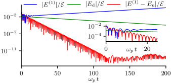
We solved the linearized Vlasov–Poisson equation numerically [9] on a periodic domain of length $L=7\lambda_{\mathrm{D}}$ with the equilibrium (12), $\sigma=v_{\mathrm{th}}/2$, $v_{0}=\sqrt{3}\,v_{\mathrm{th}}/2$, $f^{(1)}(v,0)=0.01\,f_{0}$, and $k\,\lambda_{\mathrm{D}}=2\pi/7$. Our results reveal that, contrary to Case, the decaying discrete mode is not present in the electric field; see Fig. 1. What remains after removing the unstable mode from the field (red curve) is clearly not dominated by the decaying discrete mode (green curve), but instead is the field resulting from the zeros of $\Xi^{+}$ in the lower half-plane.

To gain more insight, consider a Lorentzian two-stream equilibrium for which the solution can be readily computed in closed form. While, admittedly, this distribution is unphysical, the mathematics of the linear theory is unaffected. We take

for which

Let $\beta=\omega_{p}\sqrt{\lambda-\Lambda^{2}-1/2}$, $\lambda^{2}=1/4+2\Lambda^{2}$, and $\Lambda=k\,v_{0}/\omega_{p}$. If $v_{0}>\alpha$, then for $k<\omega_{p}\sqrt{v_{0}^{2}-\alpha^{2}}/(v_{0}^{2}+\alpha^{2})$ we have $\beta>k\,\alpha$ and $\epsilon$ has a root in the upper half-plane at $i\tilde{g}=i(\beta-k\,\alpha)$ and in the lower half-plane at $-i(\beta-k\,\alpha)$. From (19) we see that the upper half-plane root corresponds to a zero of $\Xi^{+}$ while the lower half-plane root is a zero of $\Xi^{-}$. Further, $\Xi^{+}$ has roots in the lower half-plane at frequencies $ih=-i(\beta+k\,\alpha)$ and $\pm\delta-ik\,\alpha$, where $\delta=\omega_{p}\sqrt{\lambda+\Lambda^{2}+1/2}$; these are not zeros of $\epsilon$ but of its analytic continuation and, thus, are not normal modes of the system.

Since $\Xi^{+}$ has a finite number of zeros and the integrand in (9) vanishes as $\mathop{\mathrm{Re}}\nolimits s\rightarrow-\infty$, Jackson’s method of taking the limit $\Gamma\rightarrow-\infty$ while encircling the poles gives the correct solution in this case. For this system, the integrals in the van Kampen–Case formalism can be readily computed, confirming the calculation based on (9). The electric field is

where $\widetilde{\mathcal{E}}=m\,\alpha\,\omega_{p}/q$, $\zeta_{\pm}=(\lambda\mp 2\Lambda^{2}\mp 1/2)/(\lambda\mp 4\Lambda^{2}\mp 1/2)$, and $f^{(1)}(v,0)=\mu f_{0}(v)$. (Note we choose the characteristic velocity scale to be $\alpha$ instead of the undefined $v_{th}$.) The first term in (20) is the contribution from the root of $\epsilon$ in the upper half-plane, while the remaining terms are due to zeros of $\Xi^{+}$ in the lower half-plane and represent Landau damping. A closed-form expression for $f^{(1)}(v,t)$ can be obtained but is unimportant here. The form of (20) is that of (17) and not obviously (15); no term in (20) is proportional to $e^{-\tilde{g}t}$, which would correspond to the root of $\epsilon$ in the lower half-plane. The van Kampen–Case prediction that the decaying discrete mode should be present in the solution is evidently incorrect. In the calculation it becomes clear that $E_{\mathrm{vK}}$ contains a term that exactly cancels the decaying discrete mode contribution; as we show later, this cancellation is generic.

It is convenient to rotate the complex plane in (8) with $u=is/k$ giving

where $\gamma=\Gamma/k$. The contour is now horizontal and above the poles of the integrand. The presence of the kernel $1/(u-v)$ in the integral allows us to apply well-established properties of Cauchy-type integrals [7]. We interpret (21), for $v$ real, as a “$-$” function resulting from Cauchy splitting about the Bromwich contour (recall that $\gamma>0$ and thus the real $v$-axis lies below the Bromwich contour). The strength of the method is that the Bromwich contour is left fixed and determining the unique “$+$” and “$-$” Cauchy splitting involves only algebraic manipulation of the Cauchy density (the integrand excluding the kernel). The distribution function becomes

since the first term in (21) gives

and we have defined

We find $E^{(1)}(t)$ from (5a) using (22):

Thus, the key to computing the solution is determining $\Phi^{-}$, given $F^{+}e^{-ikut}/\Xi^{+}$. Whereas $F^{\pm}$ and $\Xi^{\pm}$ are Cauchy splittings about the real axis, $\Phi^{\pm}$ are Cauchy splittings about the Bromwich contour. Thus $F^{-}$ or $\Xi^{-}$ are not used in evaluating $\Phi^{-}$; the problem is framed entirely by $F^{+}$, $\Xi^{+}$, and $e^{-ikut}$ and their respective analyticity properties.

The splitting (24) must respect the appropriate functional properties of $\Phi^{\pm}$: they must be analytic and vanish as $\mathop{\mathrm{Im}}\nolimits z\rightarrow\pm\infty$. Note, no such conditions exist for $\mathop{\mathrm{Im}}\nolimits z\rightarrow\mp\infty$. A Sokhotski relation [7] gives,

The behavior of $F^{+}$ below the real axis is the crucial fact that Jackson’s construction ignores. However, if we assume $F^{+}e^{-ikut}/\Xi^{+}$ vanishes as $\mathop{\mathrm{Im}}\nolimits u\rightarrow-\infty$ (as Jackson had done), the only singularities are from the poles of $F^{+}$ and the zeros of $\Xi^{+}$. Then, $\Phi^{\pm}$ can be deduced by a separation of the poles from $F^{+}/\Xi^{+}$:

and

where $\mathop{\mathrm{P}_{n}}\nolimits[\varphi](z)$ denotes the principal part of the Laurent series of $\varphi$ about its $n$-th pole as a function of $z$. Inserting $\Phi^{-}$ (27) into (22) and (25) gives

and

where $\mathop{\mathrm{Res}_{n}}\nolimits[\varphi]$ denotes the residue of $\varphi$ at its $n$-th pole. Note, the sums may have an infinite number of terms. Expressions (29) and (30) are the conventional Jackson result obtained by shifting and deforming the contour around the poles, which is widely cited by standard textbooks. However, this result is only correct provided $F^{+}/\Xi^{+}$ diverges more slowly than $e^{ikut}$ as $\mathop{\mathrm{Im}}\nolimits u\rightarrow-\infty$.

A Maxwellian initial condition gives an $F^{+}$ that does not generally satisfy this condition and requires a modification to the Cauchy splitting (26) and hence the solution will differ from that from Jackson’s formalism. Consider

which has essential singularities in both half-planes and can be separated as

The first (second) term on the right-hand side of (32) is analytic in the upper (lower) half-plane and vanishes at infinity but has an essential singularity at infinity in the opposite half-plane. Thus,

and separating the poles due to $\Xi^{+}$ and the singularities due to $\mathop{\mathrm{W}}\nolimits$ and $e^{-ikut}$, which require shifting the argument, allows for a Cauchy splitting (26), giving

where $b=-ka^{2}$ and $c=k^{2}a^{2}/2$. When this is inserted into (25), we find

where $\Delta$ is a constant that depends on the equilibrium. The more complicated behavior of the Maxwellian in the complex plane results in a fundamentally different Cauchy splitting and a time behavior that is not simply a sum of complex exponentials with arguments linear in time, unlike what is expected from the Jackson method. In this case, it is clear that as the Bromwich contour in (9) is shifted, $\Gamma\rightarrow-\infty$, the contour contribution to the integral does not vanish.

To illustrate the consequences of (35) we take the equilibrium

for which

and $\Delta=1$. The field is

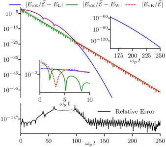
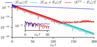
where $\eta=\sqrt{2\pi}\,\omega_{p}/ak$ and $\theta=\arg\,\mathop{\mathrm{W}}\nolimits[(ik\alpha-\omega_{p})/\sqrt{2}ak]$. The exact solution, with $\mu=0.01$, $a/\alpha=0.2$, and $k\,\alpha/\omega_{p}=1/2$, is compared with van Kampen’s solution in Fig. 2. We computed the van Kampen solution by numerically evaluating (11) using the arbitrary-precision Python library mpmath [10] carrying 200 decimal digits. We compare (11) with the analytical form (38) by fitting the electric field to $E_{\mathrm{L}}+E_{\mathrm{W}}$ where

Doing so requires surprisingly high precision since the terms involving $\mathop{\mathrm{W}}\nolimits$ are slowly varying functions of their parameters and the Gaussian-like behavior persists for some time before the exponential decay (Landau damping) associated with the single pair of roots of $\Xi^{+}$ becomes dominant. The red dashed line in the upper panel of Fig. 2 shows $E_{\mathrm{vK}}$. The blue line shows the electric field with $E_{\mathrm{L}}$ removed while the green line shows the electric field with $E_{\mathrm{W}}$ removed. The parameters extracted by the fitting reproduced the analytical values to approximately 150 digits. The fit residual, shown as the relative error in the lower panel of Fig. 2, has little structure, confirming the fitted function well-reproduces the analytical form. It is often noted that Landau damping represents the “long-time” behavior of the system. Here the field amplitude must fall by some twenty orders of magnitude before the system becomes dominated by this long-time behavior; Landau damping is almost invisible for roughly the first sixteen plasma periods. This is entirely due to contributions from the initial condition, which is in no way physically unreasonable.

It must be emphasized that the existence of non-exponential terms, i.e., those in additional to Jackson’s result, does not depend solely on the form of either the initial condition or the equilibrium, but whether $F^{+}/\Xi^{+}$ diverges more quickly than $e^{ikut}$ as $\mathop{\mathrm{Im}}\nolimits u\rightarrow-\infty$. Thus the same initial condition as above and the equilibrium

can show qualitatively the same behavior provided $a<v_{\mathrm{th}}$. For this equilibrium

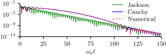
and $\Delta=3/4$. Since $\Xi^{+}$ has an infinite number of zeros, it is not possible to produce a closed-form expression for the field. The field, (35) with (41), for $a=v_{\mathrm{th}}/10$ and evaluated for the first 1000 zeros of $\Xi^{+}$ is shown as the blue curve in Fig. 3. The green curve shows Jackson’s solution evaluated with the same zeros. The dashed red curve is a numerical solution of the linearized Vlasov–Poisson equation for this equilibrium and initial condition on a periodic domain of length $L=4\pi\lambda_{\mathrm{D}}$ with $k\lambda_{\mathrm{D}}=1/2$ and $\mu=0.01$.

Further, Jackson’s method of shifting $\Gamma\rightarrow-\infty$ in (9) while analytically continuing the integrand in general does not necessarily give a reliable asymptotic approximation of the solution. Consider the above initial condition and the equilibrium

for which

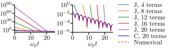
where $\psi^{(1)}$ is the trigamma function [8] and $\Delta=1$. Here Jackson’s formulation fails since the solution diverges as more terms are added, as shown in Fig. 4. The dashed red curve is a numerical solution of the linearized Vlasov–Poisson equation for this equilibrium and initial condition on a periodic domain of length $L=4\pi\lambda_{\mathrm{D}}$ with $k\lambda_{\mathrm{D}}=1/2$, $a=v_{\mathrm{th}}$, and $\mu=0.01$. The blue curve is (35) with (43) using the first 20 zeros of $\Xi^{+}$. This failure of Jackson’s formulation arises because the zeros of $\Xi^{+}$ progress down along the imaginary axis, which when evaluated in the numerator $F^{+}$ in (30) causes the amplitude to become more and more divergent. In contrast, the numerator in (35) from Cauchy splitting vanishes at infinity in the lower half-plane, resulting in a proper asymptotic form. Thus it is crucial to examine the behavior of the entire Cauchy density, not just $\Xi^{+}$ as is commonly done.

For an equilibrium with a finite collection of unstable modes of any order, the van Kampen–Case solution [2, 4, 3], in our notation, becomes

where the sums are over the zeros of $\Xi^{+}$ in the upper half-pane and $\Xi^{-}$ in the lower half-plane and P denotes the principal value. Using properties of the Cauchy splittings we have

and

which combined with Sokhotski’s relations [7],

allow us to write

When inserted into (44), the terms in the sum over $j$ in (48) exactly cancel the decaying discrete mode contributions to the distribution function, giving

It is thus apparent that Case’s counting of discrete modes [3, 4] is not correct. The decaying discrete modes, while necessarily present whenever there are growing discrete modes as part of the eigenvalue problem, always cancel with a contribution from the van Kampen modes, and thus never contribute to the time evolution of the distribution function or electric field. This result is illustrated in Fig. 5.

Elskens and Escande [11] developed a finite-degree-of-freedom particle approximation to Vlasov dynamics in the context of quasi-linear theory. They argue that an unstable/stable eigenmode pair is accompanied by Landau damping in such a way that the decaying eigenmode contribution to the electric field is cancelled by Landau damping. In distinction, while we find that the continuum does exactly cancel the decaying discrete mode, the rate of the discrete mode is significantly different than the decay rate from the Landau pole, and the same is true of the phase velocities. Our result is a rigorous property of the solution of the linearized system and not the consequence of an approximate argument.

We have developed a method for solving the linearized Vlasov–Poisson system, based on analyticity properties of the equilibrium and initial condition by exploiting properties of Cauchy-type integrals. Our method produces algebraic expressions for the distribution and field, i.e., the solution is expressed without integrals; this interpretation of (24) can be generalized to a wide class of inversion integrals. When the equilibrium results in $\Xi^{+}$ having an infinite number of zeros, our method can yield a reliable asymptotic approximation to the field and distribution function. We showed that for “reasonable” initial conditions and stable equilibria, the solution may exhibit time dependence more complicated than simple exponential decay and oscillation as expected from a naive evaluation of the inverse Laplace transform. Our analysis explained an apparent discrepancy in unstable systems between the Jackson and van Kampen–Case solutions. We showed that the contribution of decaying discrete modes to the field and distribution is always canceled by a corresponding contribution from the van Kampen modes. Case’s formulation in terms of orthogonal eigenfunctions overlooked the fact that the van Kampen modes and the decaying discrete mode eigenfunctions are not independent. As a result, Case’s “mode counting” is incorrect. Not all of the normal modes arising from solutions of $\epsilon=0$ appear in the solution; only the unstable discrete modes survive.

F.M.L. and B.A.S. contributed equally to this work.

References

- Krall and Trivelpiece [1973] N. A. Krall and A. W. Trivelpiece, Principles of Plasma Physics (McGraw-Hill New York, 1973).
- van Kampen [1955] N. G. van Kampen, On the theory of stationary waves in plasmas, Physica 21, 949 (1955).
- Case [1959] K. M. Case, Plasma oscillations, Ann. Phys. 7, 349 (1959).
- Case [1978] K. M. Case, Plasma oscillations, Phys. Fluids 21, 249 (1978).
- Jackson [1960] J. D. Jackson, Longitudinal plasma oscillations, J. Nucl. Energy C 1, 171 (1960).
- Landau [1946] L. D. Landau, On the vibration of the electronic plasma, J. Phys. USSR 10, 25 (1946), [Sov. Phys. JETP 16, 547, (1946)].
- Gakhov [1990] F. D. Gakhov, Boundary Value Problems (Dover, New York, 1990).
- Oldham et al. [2009] K. B. Oldham, J. C. Myland, and J. Spanier, An Atlas of Functions, 2nd ed. (Springer Science + Business Media, 2009).
- Carrié and Shadwick [2022] M. Carrié and B. A. Shadwick, An unconditionally stable, time-implicit algorithm for solving the one-dimensional Vlasov–Poisson system, J. Plasma Phys. 88, 905880201 (2022).
- Johansson et al. [2013] F. Johansson et al., mpmath: A Python Library for Arbitrary-Precision Floating-Point Arithmetic (Version 0.18) (2013), http://mpmath.org/.
- Elskens and Escande [2003] Y. Elskens and D. Escande, Microscopic Dynamics of Plasmas and Chaos (Institute of Physics Publishing, Bristol, UK, 2003).