This paper was converted on www.awesomepapers.org from LaTeX by an anonymous user.
Want to know more? Visit the Converter page.

A novel direct imaging method for passive inverse obstacle scattering problem

Yunwen Yin School of Mathematics, Southeast University, Nanjing, China [email protected]  and  Liang Yan School of Mathematics, Southeast University, Nanjing, China [email protected]
Abstract.

This paper investigates the inverse scattering problem of recovering a sound-soft obstacle using passive measurements taken from randomly distributed point sources. The randomness introduced by these sources poses significant challenges, leading to the failure of classical direct sampling methods that rely on scattered field measurements. To address this issue, we introduce the Doubly Cross-Correlating Method (DCM), a novel direct imaging scheme that consists of two major steps. Initially, DCM creates a cross-correlation between two passive measurements. This specially designed cross-correlation effectively handles the uncontrollability of incident sources and connects to the active scattering model via the Helmholtz-Kirchhoff identity. Subsequently, this cross-correlation is used to create a correlation-based imaging function that can qualitatively identify the obstacle. The stability and resolution of DCM are theoretically analyzed. Extensive numerical examples, including scenarios with two closely positioned obstacles and multiscale obstacles, demonstrate that DCM is computationally efficient, stable, and fast.

Keywords:   inverse obstacle scattering problem; passive imaging; direct imaging scheme; cross-correlation.

1. Introduction

Inverse scattering problems arise in many practical applications, for example, radar imaging [4], nondestructive testing [1] and medical imaging [28]. One important class of such inverse problems is the inverse obstacle scattering problem that focuses on determining the location and shape of the object. This problem is highly non-linear and severely ill-posed, which means that its solution may not exist or may not be unique, and more importantly may not be stable with respect to the noise. As a result, developing effective and stable numerical strategies is challenge but necessary. Existing reconstruction approaches can be broadly classified into three types: iterative methods, decomposition methods, and sampling-type methods. Iterative methods, such as Newton-type iterative method [26, 27] and recursive linearization method [3, 5], need to repeatedly recall the forward solver during their inversion processes, and thus they are typically faced with the curse of the high computational costs. Decomposition methods reformulate the inverse problem as a non-linear optimization problem containing two parts: the first part is to recover the scattered field from the farfield pattern, and the second part uses the boundary condition and the recovered scattered field to determine the boundary of the scatterer. It is commendable that decomposition methods are capable of not only well avoiding a sequence of forward model evaluations, but also providing satisfactory reconstructions. We refer the readers to [20, 23, 24, 37] for the relevant results of decomposition methods. Rather, sampling-type methods, also known as qualitative methods, such as the factorization method[22, 25, 38, 40], the direct sampling method [21, 32, 33, 34] and the orthogonality sampling method [36], solve the inverse obstacle scattering problem from a completely different perspective. They are devoted to designing a specific indicator function to qualitatively visualize the unknown obstacle.

The aforementioned reconstruction approaches have had enormous success with the inverse obstacle scattering problem. However, they are based on active imaging, which means that the incident field described by a time harmonic plane wave or point source is under control. Unfortunately, in many practical scenarios, the incident wave is random and unavailable, so the receivers passively record the response of the unknown impenetrable obstacle. The problem of detecting an obstacle using such passive measurements is known as passive imaging. In general, fewer studies on passive imaging have been conducted than on active imaging. In [17], a novel linear sampling method was proposed to solve inverse obstacle scattering with random sources using the Helmholtz-Kirchhoff identity and cross-correlation computed at two measurements. This work greatly contributes to the study of inverse scattering problems. Recently, the concept has been extended to passive imaging with small random scatterers [18]. We refer to [17, 18] for more detailed discussions of this method. However, because the underlying model error associated with the passive model and the approximate active model is ignored, the reconstruction will be affected accordingly. In order to overcome this, a Bayesian model error method was presented in [39] with an online estimating of the model error. We strongly recommend [19] for a comprehensive understanding of various interesting and meaningful passive inverse scattering problems. Furthermore, we would like to point out that the introduced passive problem can be solved in terms of the co-inversion of the obstacle and its excitation sources[7, 8, 41, 42].

In this work, we introduce a new direct sampling method called Doubly Cross-Correlating Method (DCM) for the passive inverse obstacle scattering with randomly distributed incident sources. The inherent randomness of these sources makes the use of scattered field data for direct detection impractical. To overcome this challenge, DCM constructs cross-correlation data from passive measurements. By leveraging the Helmholtz-Kirchhoff identity, this cross-correlation can be tightly connected to the active scattering model. Consequently, the methodologies developed for active inverse scattering problems can be utilized, leading to the establishment of a correlation-based imaging functional inspired by by the reverse time migration method [9, 10, 11, 12, 13, 14, 15, 29, 30, 31]. Specifically, we first back-propagate the well-constructed cross-correlation into the background medium and then formulate an imaging functional using the imaginary part of the cross-correlation between the fundamental solution and the back-propagated field. To the best of our knowledge, the proposed DCM represents the first approach for reconstructing impenetrable obstacles in passive imaging scenarios from a direct sampling perspective. Unlike the method presented by [17], DCM avoids solving the linear integral system. The main features and novelties of our work are summarized as follows:

  • We propose a novel direct imaging method to recover the location and shape of sound-soft obstacles in passive scenarios. This method combines cross-correlation from two passive measurements, the Helmholtz-Kirchhoff identity, and the principles of reverse time migration.

  • Instead of directly using passive measurements, we employ a specially designed cross-correlation that effectively addresses the challenges posed by the randomness and uncontrollability of incident point sources.

  • Theoretical analyses of resolution and stability are rigorously proved. Extensive numerical examples demonstrate the method’s effectiveness and efficiency. Our approach achieves satisfactory reconstructions even for complex scenarios such as two closely positioned obstacles and multiscale obstacles.

  • The proposed direct imaging method involves only matrix multiplication, making it computationally fast and simple to implement. Additionally, our method shows significant stability in the presence of noise.

The rest of the paper is organized as follows. In Section 2, the passive scattering model with randomly distributed point sources is introduced. In Section 3, the DCM for the passive inverse scattering problem is presented, along with the resolution and stability analyses. Numerical experiments are conducted in Section 4 to show the promising features of the proposed DCM. Finally, we make some conclusions in Section 5.

2. Problem setup

In this section, we shall present the mathematical descriptions of the direct and inverse scattering problem.

2.1. Direct scattering problem

Assume that D2𝐷superscript2D\subset\mathbb{R}^{2} is a bounded simply connected sound-soft obstacle with a C2superscript𝐶2C^{2}-boundary D𝐷\partial{D}. Given the time-harmonic point source located at z2D¯𝑧superscript2¯𝐷z\in\mathbb{R}^{2}\setminus\overline{D}, the incident field uisuperscript𝑢𝑖u^{i} can be described as

ui(x,z):=ϕ(x,z)=i4H0(1)(k|xz|),x2{D¯{z}},formulae-sequenceassignsuperscript𝑢𝑖𝑥𝑧italic-ϕ𝑥𝑧i4superscriptsubscript𝐻01𝑘𝑥𝑧𝑥superscript2¯𝐷𝑧\displaystyle u^{i}(x,z):=\phi(x,z)=\frac{{\mathrm{i}}}{{4}}H_{0}^{(1)}(k|x-z|),\ \ x\in\mathbb{R}^{2}\setminus\{\overline{D}\cup\{z\}\}, (2.1)

where ϕ(x,z)italic-ϕ𝑥𝑧\phi(x,z) denotes the outgoing Green function of Helmholtz equation in 2superscript2\mathbb{R}^{2}, H0(1)superscriptsubscript𝐻01H_{0}^{(1)} is the Hankel function of the first kind of order zero, k+𝑘subscriptk\in\mathbb{R}_{+} is the wave number and i:=1assigni1\mathrm{i}:=\sqrt{-1} is the imaginary unit. The presence of the sound-soft obstacle D𝐷D will interrupt the propagation of the incident wave uisuperscript𝑢𝑖u^{i}, leading to the exterior scattered field ussuperscript𝑢𝑠u^{s}. The direct scattering problem is to find us=uuisuperscript𝑢𝑠𝑢superscript𝑢𝑖u^{s}=u-u^{i} that satisfies the following Helmholtz system:

us(x,z)+k2us(x,z)=0in2\D¯,superscript𝑢𝑠𝑥𝑧superscript𝑘2superscript𝑢𝑠𝑥𝑧0\insuperscript2¯𝐷\displaystyle\bigtriangleup u^{s}(x,z)+k^{2}u^{s}(x,z)=0\ \ \mbox{in}\ \mathbb{R}^{2}\backslash\overline{D}, (2.2)
us(x,z)=ui(x,z)onD,superscript𝑢𝑠𝑥𝑧superscript𝑢𝑖𝑥𝑧on𝐷\displaystyle u^{s}(x,z)=-u^{i}(x,z)\ \ \mbox{on}\ \partial{D}, (2.3)
limr=|x|r(us(x,z)rikus(x,z))=0,subscript𝑟𝑥𝑟superscript𝑢𝑠𝑥𝑧𝑟i𝑘superscript𝑢𝑠𝑥𝑧0\displaystyle\lim_{r=|x|\rightarrow\infty}\sqrt{r}\Big{(}\frac{\partial{u^{s}(x,z)}}{\partial{r}}-\mathrm{i}ku^{s}(x,z)\Big{)}=0, (2.4)

where u𝑢u is the total field and the Sommerfeld radiation condition (2.4) describes the outgoing nature of the scattered field ussuperscript𝑢𝑠u^{s} and holds uniformly in all directions. The well-posedness of the forward scattering problem (2.2)-(2.4) is well known (cf. [16, 35]).

2.2. Passive inverse obstacle scattering problem

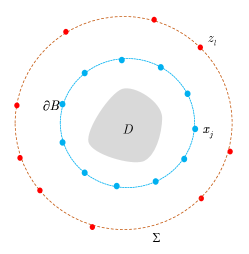
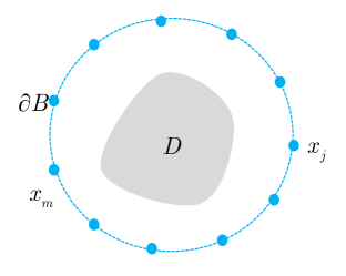
We are now going to introduce the considered passive inverse obstacle scattering problem. Let B𝐵\partial{B}, which is a circle of the radius rBsubscript𝑟𝐵r_{B} and contains D𝐷D in its interior, be the measurement curve. Measurement points xj(j=1,,J)subscript𝑥𝑗𝑗1𝐽x_{j}(j=1,\cdots,J) are located on B𝐵\partial{B}. Let zl(l=1,,L)subscript𝑧𝑙𝑙1𝐿z_{l}(l=1,\cdots,L) be the positions of incident point sources ϕ(x,zl)italic-ϕ𝑥subscript𝑧𝑙\phi(x,z_{l}) that are randomly distributed on ΣΣ\Sigma, where ΣΣ\Sigma denotes the incident curve that encloses B𝐵\partial{B}. Moreover, the random position zlsubscript𝑧𝑙z_{l} is far away from the obstacle D𝐷D. Then, the corresponding inverse problem is to determine the location and shape of the sound-soft obstacle D𝐷D from the passively collected total field u(xj,zl)𝑢subscript𝑥𝑗subscript𝑧𝑙u(x_{j},z_{l}). We refer to Fig. 1(a) for the specific illustration of this passive inverse scattering problem. In order to more intuitively describe the difference of passive imaging and active imaging, we also present illustration of active imaging in Fig. 1(b). In the active setup, measurement points xjsubscript𝑥𝑗x_{j} and source positions xmsubscript𝑥𝑚x_{m} are both controlled and located on B𝐵\partial{B}. Clearly, the main difference of these two problems is whether excitation sources are controlled. Unfortunately, we can not place active excitation sources particularly in the practical scenario that one needs to face the limitation of safety or environment, and meanwhile passive imaging viewpoint can be naturally adopted.
Refer to caption
(a) Passive imaging
Refer to caption
(b) Active imaging
Figure 1. In the passive imaging (Left), the incident sources are random and uncontrolled, but in the active imaging (Right), the incident sources are controlled and fixed.

In this paper, we want to design a direct sampling method for solving this problem. The direct sampling method has emerged as one of the most popular reconstruction techniques for inverse scattering problems due to its efficient computing capabilities. The fundamental idea is to develop a distinct imaging functional that can be used to qualitatively visualize the scatterer by applying its values at various probing points. However, in our considered passive imaging setting, directly using the scattered field us(xj,zl)superscript𝑢𝑠subscript𝑥𝑗subscript𝑧𝑙u^{s}(x_{j},z_{l}) to design the traditional direct sampling method may not be a good choice because of the randomness of the position zlsubscript𝑧𝑙z_{l}. In order to overcome this challenge, this paper proposes a novel direct imaging scheme whose specific details are presented in the following section.

3. The doubly cross-correlating method

In this section, we introduce our proposed Doubly Cross-Correlating Method (DCM) for addressing the passive inverse obstacle scattering problem. The DCM framework primarily involves two key steps: initially constructing a cross-correlation between two passive measurements, and subsequently utilizing this cross-correlation to design a correlation-based indicator functional. Essentially, our method employs a secondary imaging correlation derived from the primary data correlation computed at two passive receivers, thus aptly termed “doubly cross-correlating”. Additionally, we will present a thorough analysis of the resolution and stability of this method, highlighting its robustness and efficacy in practical applications.

3.1. DCM for the inverse problem

To describe our method, we use mathematical notations similar to works [17, 39]. Denote by ΩΩ\Omega a sampling domain that contains the obstacle D𝐷D. Before we continue, we recall ϕ(x,y)=i4H0(1)(k|xy|)italic-ϕ𝑥𝑦i4superscriptsubscript𝐻01𝑘𝑥𝑦\phi(x,y)=\frac{{\mathrm{i}}}{{4}}H_{0}^{(1)}(k|x-y|) that is the fundamental solution of the Helmholtz equation

ϕ(x,y)+k2ϕ(x,y)=δy(x)in2,italic-ϕ𝑥𝑦superscript𝑘2italic-ϕ𝑥𝑦subscript𝛿𝑦𝑥insuperscript2\displaystyle\bigtriangleup\phi(x,y)+k^{2}\phi(x,y)=-\delta_{y}(x)\ \ \mbox{in}\ \mathbb{R}^{2}, (3.1)

and satisfies the Sommerfeld radiation condition

limr=|x|r(ϕrikϕ)=0,subscript𝑟𝑥𝑟italic-ϕ𝑟i𝑘italic-ϕ0\displaystyle\lim_{r=|x|\rightarrow\infty}\sqrt{r}(\frac{\partial{\phi}}{\partial{r}}-\mathrm{i}k\phi)=0, (3.2)

where δy()subscript𝛿𝑦\delta_{y}(\cdot) is the Dirac source located at y𝑦y. In order to alleviate the difficulty caused by random sources at positions zlsubscript𝑧𝑙z_{l}, we compute the cross-correlation matrix with its entries Cjmsubscript𝐶𝑗𝑚C_{jm} defined at xjsubscript𝑥𝑗x_{j} and xmsubscript𝑥𝑚x_{m} by

Cjm=2ik|Σ|Ll=1Lu(xj,zl)¯u(xm,zl)[ϕ(xj,xm)ϕ(xj,xm)¯],1j,mJ,formulae-sequencesubscript𝐶𝑗𝑚2i𝑘Σ𝐿superscriptsubscript𝑙1𝐿¯𝑢subscript𝑥𝑗subscript𝑧𝑙𝑢subscript𝑥𝑚subscript𝑧𝑙delimited-[]italic-ϕsubscript𝑥𝑗subscript𝑥𝑚¯italic-ϕsubscript𝑥𝑗subscript𝑥𝑚formulae-sequence1𝑗𝑚𝐽\displaystyle C_{jm}=\frac{2\mathrm{i}k|\Sigma|}{L}\sum_{l=1}^{L}\overline{u\left(x_{j},z_{l}\right)}u\left(x_{m},z_{l}\right)-\left[\phi\left(x_{j},x_{m}\right)-\overline{\phi\left(x_{j},x_{m}\right)}\right],\quad 1\leq j,m\leq J, (3.3)

where |Σ|Σ|\Sigma| denotes the area of the surface ΣΣ\Sigma on which incident sources are randomly distributed, and ϕ(xj,xm)italic-ϕsubscript𝑥𝑗subscript𝑥𝑚\phi\left(x_{j},x_{m}\right) is the measurement collected at xjsubscript𝑥𝑗x_{j} of the point source located at xmsubscript𝑥𝑚x_{m}.

In what follows, we shall connect the cross-correlation (3.3) to the active scattering model. To this end, let x,y𝑥𝑦x,y be far from ΣΣ\Sigma. Then, the Helmholtz-Kirchhoff identity for ϕ(x,y)italic-ϕ𝑥𝑦\phi(x,y) is described as [17, 39]

ϕ(x,y)ϕ(x,y)¯=2ikΣϕ(x,z)¯ϕ(y,z)ds(z).italic-ϕ𝑥𝑦¯italic-ϕ𝑥𝑦2i𝑘subscriptΣ¯italic-ϕ𝑥𝑧italic-ϕ𝑦𝑧differential-d𝑠𝑧\displaystyle\phi(x,y)-\overline{\phi(x,y)}=2\mathrm{i}k\int_{\Sigma}\overline{\phi(x,z)}\phi(y,z)\mathrm{d}s(z). (3.4)

We remark that (3.4) holds for the case that x𝑥x and y𝑦y are far from ΣΣ\Sigma, namely for zΣ𝑧Σz\in\Sigma, |xz|𝑥𝑧|x-z| and |yz|𝑦𝑧|y-z| are both required to be large enough. Viewing ϕ(x,y)italic-ϕ𝑥𝑦\phi(x,y) as the incident source located at y𝑦y, the corresponding total field measured at x𝑥x is given by u(x,y)=ϕ(x,y)+us(x,y)𝑢𝑥𝑦italic-ϕ𝑥𝑦superscript𝑢𝑠𝑥𝑦u(x,y)=\phi(x,y)+u^{s}(x,y). The Helmholtz-Kirchhoff identity also holds for u(x,y)𝑢𝑥𝑦u(x,y) [17, 39], that is,

u(x,y)u(x,y)¯=2ikΣu(x,z)¯u(y,z)ds(z).𝑢𝑥𝑦¯𝑢𝑥𝑦2i𝑘subscriptΣ¯𝑢𝑥𝑧𝑢𝑦𝑧differential-d𝑠𝑧\displaystyle u(x,y)-\overline{u(x,y)}=2\mathrm{i}k\int_{\Sigma}\overline{u(x,z)}u(y,z)\mathrm{d}s(z). (3.5)

The formulas (3.4) and (3.5) immediately give rise to

us(x,y)us(x,y)¯=2ikΣu(x,z)¯u(y,z)ds(z)[ϕ(x,y)ϕ(x,y)¯].superscript𝑢𝑠𝑥𝑦¯superscript𝑢𝑠𝑥𝑦2i𝑘subscriptΣ¯𝑢𝑥𝑧𝑢𝑦𝑧differential-d𝑠𝑧delimited-[]italic-ϕ𝑥𝑦¯italic-ϕ𝑥𝑦\displaystyle u^{s}(x,y)-\overline{u^{s}(x,y)}=2\mathrm{i}k\int_{\Sigma}\overline{u(x,z)}u(y,z)\mathrm{d}s(z)-[\phi(x,y)-\overline{\phi(x,y)}]. (3.6)

By replacing x𝑥x and y𝑦y by xjsubscript𝑥𝑗x_{j} and xmsubscript𝑥𝑚x_{m} respectively, we obtain

us(xj,xm)us(xj,xm)¯=2ikΣu(xj,z)¯u(xm,z)ds(z)[ϕ(xj,xm)ϕ(xj,xm)¯].superscript𝑢𝑠subscript𝑥𝑗subscript𝑥𝑚¯superscript𝑢𝑠subscript𝑥𝑗subscript𝑥𝑚2i𝑘subscriptΣ¯𝑢subscript𝑥𝑗𝑧𝑢subscript𝑥𝑚𝑧differential-d𝑠𝑧delimited-[]italic-ϕsubscript𝑥𝑗subscript𝑥𝑚¯italic-ϕsubscript𝑥𝑗subscript𝑥𝑚\displaystyle u^{s}(x_{j},x_{m})-\overline{u^{s}(x_{j},x_{m})}=2\mathrm{i}k\int_{\Sigma}\overline{u(x_{j},z)}u(x_{m},z)\mathrm{d}s(z)-[\phi(x_{j},x_{m})-\overline{\phi(x_{j},x_{m})}]. (3.7)

Note that us(xj,xm)superscript𝑢𝑠subscript𝑥𝑗subscript𝑥𝑚u^{s}(x_{j},x_{m}) can be regarded as the active scattered field measured at xjsubscript𝑥𝑗x_{j} due to the illumination by an active source located at xmsubscript𝑥𝑚x_{m}. For the sake of the following use, we define

Njms=us(xj,xm)us(xj,xm)¯,1j,mJ.formulae-sequencesubscriptsuperscript𝑁𝑠𝑗𝑚superscript𝑢𝑠subscript𝑥𝑗subscript𝑥𝑚¯superscript𝑢𝑠subscript𝑥𝑗subscript𝑥𝑚formulae-sequence1𝑗𝑚𝐽\displaystyle N^{s}_{jm}=u^{s}(x_{j},x_{m})-\overline{u^{s}(x_{j},x_{m})},\quad 1\leq j,m\leq J. (3.8)

Therefore, the relationship between the cross-correlation (3.3) and the imaginary scattered field (3.8) is

CjmNjms.subscript𝐶𝑗𝑚subscriptsuperscript𝑁𝑠𝑗𝑚\displaystyle C_{jm}\approx N^{s}_{jm}. (3.9)

In fact, (3.3) is the discrete approximation form of (3.8), and the approximation accuracy between these two parts relies on the total number L𝐿L and the random position zlsubscript𝑧𝑙z_{l}. See Fig. 1(b) for the illustration of the introduced active scattering problem.

Before we proceed, let us explain why traditional direct sampling methods will fail in passive imaging. Indeed, traditional direct sampling methods are constructed by using the scattered field us(xj,zl)superscript𝑢𝑠subscript𝑥𝑗subscript𝑧𝑙u^{s}(x_{j},z_{l}), but in passive imaging setup only total field u(xj,zl)𝑢subscript𝑥𝑗subscript𝑧𝑙u(x_{j},z_{l}) is accessible and the scattered field can not be attainable due to the randomness of zlsubscript𝑧𝑙z_{l}. Even though one can have us(xj,zl)superscript𝑢𝑠subscript𝑥𝑗subscript𝑧𝑙u^{s}(x_{j},z_{l}), the influence of randomness of zlsubscript𝑧𝑙z_{l} still exists. To show this, we write the indicator functional of classical reverse time migration method by using us(xj,zl)superscript𝑢𝑠subscript𝑥𝑗subscript𝑧𝑙u^{s}(x_{j},z_{l}), which is in the form

IRTM(τ)=k2Im{2πrB|Σ|Jl=1Lj=1Jϕ(τ,zl)ϕ(τ,xj)us(xj,zl)¯},subscript𝐼𝑅𝑇𝑀𝜏superscript𝑘2Im2𝜋subscript𝑟𝐵Σ𝐽superscriptsubscript𝑙1𝐿superscriptsubscript𝑗1𝐽italic-ϕ𝜏subscript𝑧𝑙italic-ϕ𝜏subscript𝑥𝑗¯superscript𝑢𝑠subscript𝑥𝑗subscript𝑧𝑙\displaystyle I_{RTM}(\tau)=-k^{2}\mathrm{Im}\left\{\frac{2\pi r_{B}|\Sigma|}{J}\sum\limits_{l=1}^{L}\sum\limits_{j=1}^{J}\phi(\tau,z_{l})\phi(\tau,x_{j})\overline{u^{s}(x_{j},z_{l})}\right\}, (3.10)

where τΩ𝜏Ω\tau\in\Omega is the sampling point. Clearly, in the imaging process this indicator (3.10) shall inevitably fail since positions zlsubscript𝑧𝑙z_{l} are unknown. The above discussed two issues of traditional direct sampling approaches can be overcome by employing (3.3) instead of us(xj,zl)superscript𝑢𝑠subscript𝑥𝑗subscript𝑧𝑙u^{s}(x_{j},z_{l}). Thus in what follows, we shall introduce the specific design of our imaging functional. Because of the approximation relationship (3.9), we can naturally benefit from the existing active imaging methods. Comparable to the reverse time migration method, our imaging algorithm contains two phases. The first phase is the back-propagation stage in which the complex conjugated data Cjm¯¯subscript𝐶𝑗𝑚\overline{C_{jm}} is back-propagated into the domain. Specifically, for m=1,2,,J𝑚12𝐽m=1,2,\cdots,J, we compute the solution vbsubscript𝑣𝑏v_{b} to the following problem:

vb(x,xm)+k2vb(x,xm)=2πrBJj=1JCjm¯δxj(x)in2,subscript𝑣𝑏𝑥subscript𝑥𝑚superscript𝑘2subscript𝑣𝑏𝑥subscript𝑥𝑚2𝜋subscript𝑟𝐵𝐽superscriptsubscript𝑗1𝐽¯subscript𝐶𝑗𝑚subscript𝛿subscript𝑥𝑗𝑥insuperscript2\displaystyle\bigtriangleup v_{b}(x,x_{m})+k^{2}v_{b}(x,x_{m})=\frac{2\pi r_{B}}{J}\sum\limits_{j=1}^{J}\overline{C_{jm}}\delta_{x_{j}}(x)\ \ \mbox{in}\ \mathbb{R}^{2}, (3.11)
limr=|x|r(vbrikvb)=0.subscript𝑟𝑥𝑟subscript𝑣𝑏𝑟i𝑘subscript𝑣𝑏0\displaystyle\lim_{r=|x|\rightarrow\infty}\sqrt{r}(\frac{\partial{v_{b}}}{\partial{r}}-\mathrm{i}kv_{b})=0. (3.12)

By (3.1), (3.2) and the linearity, the solution vbsubscript𝑣𝑏v_{b} to (3.11) and (3.12) can be represented by

vb(x,xm)=2πrBJj=1JCjm¯ϕ(x,xj).subscript𝑣𝑏𝑥subscript𝑥𝑚2𝜋subscript𝑟𝐵𝐽superscriptsubscript𝑗1𝐽¯subscript𝐶𝑗𝑚italic-ϕ𝑥subscript𝑥𝑗\displaystyle v_{b}(x,x_{m})=-\frac{2\pi r_{B}}{J}\sum\limits_{j=1}^{J}\overline{C_{jm}}\phi(x,x_{j}). (3.13)

Then for τΩ𝜏Ω\tau\in\Omega, the imaginary part of the cross-correlation of the fundamental solution ϕ(τ,xm)italic-ϕ𝜏subscript𝑥𝑚\phi(\tau,x_{m}) and the back-propagated field vb(τ,xm)subscript𝑣𝑏𝜏subscript𝑥𝑚v_{b}(\tau,x_{m}) is employed in the second phase, which has the form

I(τ)𝐼𝜏\displaystyle I(\tau) =k2Im{2πrBJm=1Jϕ(τ,xm)vb(τ,xm)}absentsuperscript𝑘2Im2𝜋subscript𝑟𝐵𝐽superscriptsubscript𝑚1𝐽italic-ϕ𝜏subscript𝑥𝑚superscript𝑣𝑏𝜏subscript𝑥𝑚\displaystyle=k^{2}\mathrm{Im}\left\{\frac{2\pi r_{B}}{J}\sum\limits_{m=1}^{J}\phi(\tau,x_{m})v^{b}(\tau,x_{m})\right\} (3.14)
=k2Im{(2π)2rB2J2m=1Jj=1Jϕ(τ,xm)ϕ(τ,xj)Cjm¯}.absentsuperscript𝑘2Imsuperscript2𝜋2superscriptsubscript𝑟𝐵2superscript𝐽2superscriptsubscript𝑚1𝐽superscriptsubscript𝑗1𝐽italic-ϕ𝜏subscript𝑥𝑚italic-ϕ𝜏subscript𝑥𝑗¯subscript𝐶𝑗𝑚\displaystyle=-k^{2}\mathrm{Im}\left\{\frac{(2\pi)^{2}r_{B}^{2}}{J^{2}}\sum\limits_{m=1}^{J}\sum\limits_{j=1}^{J}\phi(\tau,x_{m})\phi(\tau,x_{j})\overline{C_{jm}}\right\}.

The formula (3.14) is the main imaging functional of the proposed DCM. (3.3) and (3.14) are the so-called two cross-correlations of DCM.

3.2. The resolution analysis and stability analysis

In this subsection, we first investigate the resolution analysis of the proposed DCM, which aims to show different properties of indicator functional (3.14) when probing point τ𝜏\tau approaches the boundary D𝐷\partial D and goes away from D𝐷\partial D. To this end, in the following we estimate the bound of (3.14) when τ𝜏\tau changes. Then we further study the stability analysis that indicates our DCM is robust to the added noise. Considering the relationship (3.9), we define

INs(τ)=k2Im{(2π)2rB2J2m=1Jj=1Jϕ(τ,xm)ϕ(τ,xj)Njms¯}.subscript𝐼superscript𝑁𝑠𝜏superscript𝑘2Imsuperscript2𝜋2superscriptsubscript𝑟𝐵2superscript𝐽2superscriptsubscript𝑚1𝐽superscriptsubscript𝑗1𝐽italic-ϕ𝜏subscript𝑥𝑚italic-ϕ𝜏subscript𝑥𝑗¯subscriptsuperscript𝑁𝑠𝑗𝑚\displaystyle I_{N^{s}}(\tau)=-k^{2}\mathrm{Im}\left\{\frac{(2\pi)^{2}r_{B}^{2}}{J^{2}}\sum\limits_{m=1}^{J}\sum\limits_{j=1}^{J}\phi(\tau,x_{m})\phi(\tau,x_{j})\overline{N^{s}_{jm}}\right\}. (3.15)

If the sampling point τ𝜏\tau is contained inside the curve B𝐵\partial{B}, then ϕ(τ,xj)italic-ϕ𝜏subscript𝑥𝑗\phi(\tau,x_{j}) and ϕ(τ,xm)italic-ϕ𝜏subscript𝑥𝑚\phi(\tau,x_{m}) are both smooth functions. Furthermore, the imaginary scattered field Njmssubscriptsuperscript𝑁𝑠𝑗𝑚N^{s}_{jm} is also smooth. As a result, INssubscript𝐼superscript𝑁𝑠I_{N^{s}} can be regarded as the discrete approximation of the following continuous indicator function:

I^Ns(τ)subscript^𝐼superscript𝑁𝑠𝜏\displaystyle\hat{I}_{N^{s}}(\tau) =k2ImBBϕ(τ,xm)ϕ(τ,xj)Njms¯ds(xm)ds(xj)absentsuperscript𝑘2Imsubscript𝐵subscript𝐵italic-ϕ𝜏subscript𝑥𝑚italic-ϕ𝜏subscript𝑥𝑗¯subscriptsuperscript𝑁𝑠𝑗𝑚differential-d𝑠subscript𝑥𝑚differential-d𝑠subscript𝑥𝑗\displaystyle=-k^{2}\mathrm{Im}\int_{\partial{B}}\int_{\partial{B}}\phi(\tau,x_{m})\phi(\tau,x_{j})\overline{N^{s}_{jm}}\mathrm{d}s(x_{m})\mathrm{d}s(x_{j}) (3.16)
=k2ImBBϕ(τ,xm)ϕ(τ,xj)us(xj,xm)¯ds(xm)ds(xj)absentsuperscript𝑘2Imsubscript𝐵subscript𝐵italic-ϕ𝜏subscript𝑥𝑚italic-ϕ𝜏subscript𝑥𝑗¯superscript𝑢𝑠subscript𝑥𝑗subscript𝑥𝑚differential-d𝑠subscript𝑥𝑚differential-d𝑠subscript𝑥𝑗\displaystyle=-k^{2}\mathrm{Im}\int_{\partial{B}}\int_{\partial{B}}\phi(\tau,x_{m})\phi(\tau,x_{j})\overline{u^{s}(x_{j},x_{m})}\mathrm{d}s(x_{m})\mathrm{d}s(x_{j})
+k2ImBBϕ(τ,xm)ϕ(τ,xj)us(xj,xm)ds(xm)ds(xj).superscript𝑘2Imsubscript𝐵subscript𝐵italic-ϕ𝜏subscript𝑥𝑚italic-ϕ𝜏subscript𝑥𝑗superscript𝑢𝑠subscript𝑥𝑗subscript𝑥𝑚differential-d𝑠subscript𝑥𝑚differential-d𝑠subscript𝑥𝑗\displaystyle+k^{2}\mathrm{Im}\int_{\partial{B}}\int_{\partial{B}}\phi(\tau,x_{m})\phi(\tau,x_{j})u^{s}(x_{j},x_{m})\mathrm{d}s(x_{m})\mathrm{d}s(x_{j}).

Clearly, the first term at the right hand side of (3.16) is the standard indicator of reverse time migration method that is presented in [9]. Its analysis is also thoroughly studied in [9]. Thus, for the following resolution analysis, we mainly focus on estimating the second term. To this end, we first present some lemmas for the following use.

Lemma 3.1 ([16, 35]).

Let ω~H1/2(D)~𝜔superscript𝐻12𝐷\widetilde{\omega}\in H^{1/2}(\partial D), the forward obstacle scattering problem:

ω+k2ω=0in2\D¯,ω=ω~onD,formulae-sequence𝜔superscript𝑘2𝜔0\insuperscript2¯𝐷𝜔~𝜔on𝐷\displaystyle\bigtriangleup\omega+k^{2}\omega=0\ \ \mbox{in}\ \mathbb{R}^{2}\backslash\overline{D},\ \ \omega=\widetilde{\omega}\ \ \mbox{on}\ \partial{D}, (3.17)
limr=|x|r(ωrikω)=0,subscript𝑟𝑥𝑟𝜔𝑟i𝑘𝜔0\displaystyle\lim_{r=|x|\rightarrow\infty}\sqrt{r}(\frac{\partial{\omega}}{\partial{r}}-\mathrm{i}k\omega)=0, (3.18)

admits a unique solution ωHloc1(2\D¯)𝜔subscriptsuperscript𝐻1𝑙𝑜𝑐\superscript2¯𝐷\omega\in H^{1}_{loc}(\mathbb{R}^{2}\backslash\overline{D}). Furthermore, there exists a constant C+𝐶subscriptC\in\mathbb{R}_{+} such that

ωνH1/2(D)Cω~H1/2(D),subscriptnorm𝜔𝜈superscript𝐻12𝐷𝐶subscriptnorm~𝜔superscript𝐻12𝐷\displaystyle\left\|\frac{\partial\omega}{\partial\nu}\right\|_{H^{-1/2}(\partial D)}\leq C\|\widetilde{\omega}\|_{H^{1/2}(\partial D)},

where ν𝜈\nu denotes the unit outer normal to D𝐷\partial D.

Lemma 3.1 depicts the well-posedness of the forward scattering problem. We refer to [16, 35] for more relevant discussions. Define the Dirichlet-to-Neumann mapping T:H1/2(D)H1/2(D):𝑇superscript𝐻12𝐷superscript𝐻12𝐷T:H^{1/2}(\partial D)\rightarrow H^{-1/2}(\partial D) for any ω~H1/2(D)~𝜔superscript𝐻12𝐷\widetilde{\omega}\in H^{1/2}(\partial D) by T(ω~)=ων𝑇~𝜔𝜔𝜈T(\widetilde{\omega})=\frac{\partial\omega}{\partial\nu}. It follows from Lemma 3.1 that T𝑇T is a bounded linear operator. Denote the norm by Tnorm𝑇\|T\|. Since the obstacle D𝐷D and the sampling point τ𝜏\tau are both contained inside B𝐵\partial B, we define h1=dist(B,D)subscript1dist𝐵𝐷h_{1}=\mathrm{dist}(\partial{B},\partial{D}) and h2=dist(τ,B)subscript2dist𝜏𝐵h_{2}=\mathrm{dist}(\tau,\partial{B}). The following lemma on the estimation of the second term at the right hand side of (3.16) holds.

Lemma 3.2.

There exists constants M1,M2>0subscript𝑀1subscript𝑀20M_{1},M_{2}>0 such that

|k2ImBBϕ(τ,xm)ϕ(τ,xj)us(xj,xm)ds(xm)ds(xj)|superscript𝑘2Imsubscript𝐵subscript𝐵italic-ϕ𝜏subscript𝑥𝑚italic-ϕ𝜏subscript𝑥𝑗superscript𝑢𝑠subscript𝑥𝑗subscript𝑥𝑚differential-d𝑠subscript𝑥𝑚differential-d𝑠subscript𝑥𝑗\displaystyle\left|k^{2}\mathrm{Im}\int_{\partial{B}}\int_{\partial{B}}\phi(\tau,x_{m})\phi(\tau,x_{j})u^{s}(x_{j},x_{m})\mathrm{d}s(x_{m})\mathrm{d}s(x_{j})\right| (3.19)
M1(1+T)rB2(h1h2)1+M2rB2k1/2h13/2h21,absentsubscript𝑀11norm𝑇subscriptsuperscript𝑟2𝐵superscriptsubscript1subscript21subscript𝑀2subscriptsuperscript𝑟2𝐵superscript𝑘12superscriptsubscript132superscriptsubscript21\displaystyle\leq M_{1}(1+\|T\|)r^{2}_{B}(h_{1}h_{2})^{-1}+M_{2}r^{2}_{B}k^{-1/2}h_{1}^{-3/2}h_{2}^{-1},

where M1subscript𝑀1M_{1} and M2subscript𝑀2M_{2} are independent of k𝑘k, h1subscript1h_{1}, h2subscript2h_{2}, Tnorm𝑇\|T\| and rBsubscript𝑟𝐵r_{B} but depends on the size of D𝐷D.

Proof.

From [14, 6], we obtain

|H0(1)(t)|2πt,|H1(1)(t)|2πt+2πt,t>0,formulae-sequencesuperscriptsubscript𝐻01𝑡2𝜋𝑡formulae-sequencesuperscriptsubscript𝐻11𝑡2𝜋𝑡2𝜋𝑡for-all𝑡0\displaystyle|H_{0}^{(1)}(t)|\leq\sqrt{\frac{2}{\pi t}},\quad\quad|H_{1}^{(1)}(t)|\leq\sqrt{\frac{2}{\pi t}}+\frac{2}{\pi t},\quad\forall t>0, (3.20)

where H0(1)superscriptsubscript𝐻01H_{0}^{(1)} is the Hankel function of the first kind of order zero and H1(1)superscriptsubscript𝐻11H_{1}^{(1)} is the Hankel function of the first kind of the first order. By the integral representation formula, the scattered field us(xj,xm)superscript𝑢𝑠subscript𝑥𝑗subscript𝑥𝑚u^{s}(x_{j},x_{m}) is given as

us(xj,xm)=D(us(y,xm)ϕ(xj,y)ν(y)us(y,xm)ν(y)ϕ(xj,y))ds(y).superscript𝑢𝑠subscript𝑥𝑗subscript𝑥𝑚subscript𝐷superscript𝑢𝑠𝑦subscript𝑥𝑚italic-ϕsubscript𝑥𝑗𝑦𝜈𝑦superscript𝑢𝑠𝑦subscript𝑥𝑚𝜈𝑦italic-ϕsubscript𝑥𝑗𝑦differential-d𝑠𝑦\displaystyle u^{s}(x_{j},x_{m})=\int_{\partial D}\left(u^{s}(y,x_{m})\frac{\partial\phi(x_{j},y)}{\partial\nu(y)}-\frac{\partial u^{s}(y,x_{m})}{\partial\nu(y)}\phi(x_{j},y)\right)\mathrm{d}s(y). (3.21)

Combining (3.20), (3.21) and the fact that us(y,xm)|yD=ϕ(y,xm)|yDevaluated-atsuperscript𝑢𝑠𝑦subscript𝑥𝑚𝑦𝐷evaluated-atitalic-ϕ𝑦subscript𝑥𝑚𝑦𝐷u^{s}(y,x_{m})|_{y\in\partial D}=-\phi(y,x_{m})|_{y\in\partial D}, we have

|us(xj,xm)|superscript𝑢𝑠subscript𝑥𝑗subscript𝑥𝑚\displaystyle|u^{s}(x_{j},x_{m})| |D|8π(1+T)(k|xmy|)1/2(k|xjy|)1/2absent𝐷8𝜋1norm𝑇superscript𝑘subscript𝑥𝑚𝑦12superscript𝑘subscript𝑥𝑗𝑦12\displaystyle\leq\frac{|\partial D|}{8\pi}(1+\|T\|)(k|x_{m}-y|)^{-1/2}(k|x_{j}-y|)^{-1/2} (3.22)
+2π|D|8π2(k|xmy|)1/2(k|xjy|)12𝜋𝐷8superscript𝜋2superscript𝑘subscript𝑥𝑚𝑦12superscript𝑘subscript𝑥𝑗𝑦1\displaystyle\quad\quad+\frac{\sqrt{2\pi}|\partial D|}{8\pi^{2}}(k|x_{m}-y|)^{-1/2}(k|x_{j}-y|)^{-1}
|D|8π(1+T)(kh1)1+2π|D|8π2(kh1)3/2.absent𝐷8𝜋1norm𝑇superscript𝑘subscript112𝜋𝐷8superscript𝜋2superscript𝑘subscript132\displaystyle\leq\frac{|\partial D|}{8\pi}(1+\|T\|)(kh_{1})^{-1}+\frac{\sqrt{2\pi}|\partial D|}{8\pi^{2}}(kh_{1})^{-3/2}.

By (3.22) and again using (3.20), we have

|k2ImBBϕ(τ,xm)ϕ(τ,xj)us(xj,xm)ds(xm)ds(xj)|superscript𝑘2Imsubscript𝐵subscript𝐵italic-ϕ𝜏subscript𝑥𝑚italic-ϕ𝜏subscript𝑥𝑗superscript𝑢𝑠subscript𝑥𝑗subscript𝑥𝑚differential-d𝑠subscript𝑥𝑚differential-d𝑠subscript𝑥𝑗\displaystyle\left|k^{2}\mathrm{Im}\int_{\partial{B}}\int_{\partial{B}}\phi(\tau,x_{m})\phi(\tau,x_{j})u^{s}(x_{j},x_{m})\mathrm{d}s(x_{m})\mathrm{d}s(x_{j})\right|
\displaystyle\leq |D|16(1+T)rB2h11|τxm|1/2|τxj|1/2𝐷161norm𝑇subscriptsuperscript𝑟2𝐵superscriptsubscript11superscript𝜏subscript𝑥𝑚12superscript𝜏subscript𝑥𝑗12\displaystyle\frac{|\partial D|}{16}(1+\|T\|)r^{2}_{B}h_{1}^{-1}|\tau-x_{m}|^{-1/2}|\tau-x_{j}|^{-1/2}
+2π|D|16πrB2k1/2h13/2|τxm|1/2|τxj|1/2.2𝜋𝐷16𝜋subscriptsuperscript𝑟2𝐵superscript𝑘12superscriptsubscript132superscript𝜏subscript𝑥𝑚12superscript𝜏subscript𝑥𝑗12\displaystyle\quad\quad+\frac{\sqrt{2\pi}|\partial D|}{16\pi}r^{2}_{B}k^{-1/2}h_{1}^{-3/2}|\tau-x_{m}|^{-1/2}|\tau-x_{j}|^{-1/2}.

Then, we can derive the estimate (3.19). This completes the proof. ∎

Now, we are ready to present our main results.

Theorem 3.1.

For the sampling point τΩ𝜏Ω\tau\in\Omega that is located inside B𝐵\partial B, let ψ(x,τ)𝜓𝑥𝜏\psi(x,\tau) be the radiation solution of the Helmholtz equation

ψ(x,τ)+k2ψ(x,τ)=0in2\D¯,ψ(x,τ)=Imϕ(x,τ)onD.formulae-sequence𝜓𝑥𝜏superscript𝑘2𝜓𝑥𝜏0\insuperscript2¯𝐷𝜓𝑥𝜏Imitalic-ϕ𝑥𝜏on𝐷\displaystyle\bigtriangleup\psi(x,\tau)+k^{2}\psi(x,\tau)=0\ \ \mbox{in}\ \mathbb{R}^{2}\backslash\overline{D},\ \ \psi(x,\tau)=-\mathrm{Im}\phi(x,\tau)\ \ \mbox{on}\ \partial{D}. (3.23)

Assume that the position zlsubscript𝑧𝑙z_{l} of the random incident source is ξ𝜉\xi-perturbed, where ξ𝜉\xi denotes the perturbation value. Then for 0<ξ<1/20𝜉120<\xi<1/2, I(τ)𝐼𝜏I(\tau) defined in (3.14) satisfies that

I(τ)=kS|ψ(x^,τ)|2dx^+R(τ),𝐼𝜏𝑘subscript𝑆superscriptsuperscript𝜓^𝑥𝜏2differential-d^𝑥𝑅𝜏\displaystyle I(\tau)=k\int_{S}|\psi^{\infty}(\hat{x},\tau)|^{2}\mathrm{d}\hat{x}+R(\tau), (3.24)

where S:={x^2:|x^|=1}assign𝑆conditional-set^𝑥superscript2^𝑥1S:=\left\{\hat{x}\in\mathbb{R}^{2}:|\hat{x}|=1\right\} and R(τ)𝑅𝜏R(\tau) is the remainder term that satisfies

|R(τ)|M1(1+T)rB2(h1h2)1+M2rB2k1/2h13/2h21+M3L24ξ+M4J+M5rB1,𝑅𝜏subscript𝑀11norm𝑇subscriptsuperscript𝑟2𝐵superscriptsubscript1subscript21subscript𝑀2subscriptsuperscript𝑟2𝐵superscript𝑘12superscriptsubscript132superscriptsubscript21subscript𝑀3superscript𝐿24𝜉subscript𝑀4𝐽subscript𝑀5superscriptsubscript𝑟𝐵1\displaystyle|R(\tau)|\leq M_{1}(1+\|T\|)r^{2}_{B}(h_{1}h_{2})^{-1}+M_{2}r^{2}_{B}k^{-1/2}h_{1}^{-3/2}h_{2}^{-1}+\frac{M_{3}}{L^{2-4\xi}}+\frac{M_{4}}{J}+M_{5}r_{B}^{-1}, (3.25)

where L𝐿L is the number of incident sources, J𝐽J is the number of measurement points, M1,M2,M3,M4,M5subscript𝑀1subscript𝑀2subscript𝑀3subscript𝑀4subscript𝑀5M_{1},M_{2},M_{3},M_{4},M_{5} are all positive constants and M1,M2subscript𝑀1subscript𝑀2M_{1},M_{2} are defined in (3.19).

Proof.

For 0<ξ<1/20𝜉120<\xi<1/2, by Theorem 1 in [2] and the fact that the scattered field ussuperscript𝑢𝑠u^{s} is twice continuously differentiable, we have

|NjmsCjm|=O(1L24ξ).subscriptsuperscript𝑁𝑠𝑗𝑚subscript𝐶𝑗𝑚𝑂1superscript𝐿24𝜉\displaystyle|N^{s}_{jm}-C_{jm}|=O(\frac{1}{L^{2-4\xi}}). (3.26)

Moreover, since (3.15) is the trapezoid quadrature approximation of (3.16), and ϕ(τ,xj)italic-ϕ𝜏subscript𝑥𝑗\phi(\tau,x_{j}), ϕ(τ,xm)italic-ϕ𝜏subscript𝑥𝑚\phi(\tau,x_{m}), Njmssubscriptsuperscript𝑁𝑠𝑗𝑚N^{s}_{jm} are all smooth functions, it follows that

|INs(τ)I^Ns(τ)|subscript𝐼superscript𝑁𝑠𝜏subscript^𝐼superscript𝑁𝑠𝜏\displaystyle|I_{N^{s}}(\tau)-\hat{I}_{N^{s}}(\tau)| (3.27)
=|12(2π)3Jd(ϕ(τ,x)ϕ(τ,y)us(x,y)us(x,y)¯¯)dx|(x,y)=(ζ1,ζ2)absentsubscript12superscript2𝜋3𝐽ditalic-ϕ𝜏𝑥italic-ϕ𝜏𝑦¯superscript𝑢𝑠𝑥𝑦¯superscript𝑢𝑠𝑥𝑦d𝑥𝑥𝑦subscript𝜁1subscript𝜁2\displaystyle=|\frac{1}{2}\frac{(2\pi)^{3}}{J}\frac{\mathrm{d}(\phi(\tau,x)\phi(\tau,y)\overline{u^{s}(x,y)-\overline{u^{s}(x,y)}})}{\mathrm{d}x}|_{(x,y)=(\zeta_{1},\zeta_{2})}
+12(2π)3Jd(ϕ(τ,x)ϕ(τ,y)us(x,y)us(x,y)¯¯)dy|(x,y)=(ζ3,ζ4)|\displaystyle\quad\quad\quad+\frac{1}{2}\frac{(2\pi)^{3}}{J}\frac{\mathrm{d}(\phi(\tau,x)\phi(\tau,y)\overline{u^{s}(x,y)-\overline{u^{s}(x,y)}})}{\mathrm{d}y}|_{(x,y)=(\zeta_{3},\zeta_{4})}|
=O(1J).absent𝑂1𝐽\displaystyle=O(\frac{1}{J}).

Then, combining Theorem 3.3 of [9], (3.26), (3.27), Lemma 3.2, we obtain

I(τ)=kS|ψ(x^,τ)|2dx^+R(τ),𝐼𝜏𝑘subscript𝑆superscriptsuperscript𝜓^𝑥𝜏2differential-d^𝑥𝑅𝜏\displaystyle I(\tau)=k\int_{S}|\psi^{\infty}(\hat{x},\tau)|^{2}\mathrm{d}\hat{x}+R(\tau),

and R(τ)𝑅𝜏R(\tau) satisfies (3.25). The proof is completed. ∎

Remark 3.1.

Theorem 3.1 indicates that the indicator functional (3.14) has the contrast at the boundary D𝐷\partial D and decays when the sampling point τ𝜏\tau goes away from the obstacle D𝐷D. Additionally, we would like to point out that, Theorem 3.1 holds for 0<ξ<1/20𝜉120<\xi<1/2 primarily due to (3.26). Nonetheless, numerical experiments presented in Section 4 show that our proposed approach also works well for the case of ξ1/2𝜉12\xi\geq 1/2.

Let h~1=dist(D,Σ)subscript~1dist𝐷Σ\widetilde{h}_{1}=\mathrm{dist}(\partial{D},\Sigma) and h~2=dist(B,Σ)subscript~2dist𝐵Σ\widetilde{h}_{2}=\mathrm{dist}(\partial{B},\Sigma) respectively be distances of D𝐷\partial D to ΣΣ\Sigma and B𝐵\partial B to ΣΣ\Sigma. The following stability result holds.

Theorem 3.2.

There exist positive constants M6subscript𝑀6M_{6} and M7subscript𝑀7M_{7} that are independent of the sampling point τ𝜏\tau such that

|I(τ)Iδ(τ)|M6uδ(x,z)u(x,z)L(B×Σ)2+M7uδ(x,z)u(x,z)L(B×Σ),𝐼𝜏superscript𝐼𝛿𝜏subscript𝑀6subscriptsuperscriptnormsuperscript𝑢𝛿𝑥𝑧𝑢𝑥𝑧2superscript𝐿𝐵Σsubscript𝑀7subscriptnormsuperscript𝑢𝛿𝑥𝑧𝑢𝑥𝑧superscript𝐿𝐵Σ\displaystyle\left|I(\tau)-I^{\delta}(\tau)\right|\leq M_{6}\|u^{\delta}(x,z)-u(x,z)\|^{2}_{L^{\infty}(\partial B\times\Sigma)}+M_{7}\|u^{\delta}(x,z)-u(x,z)\|_{L^{\infty}(\partial B\times\Sigma)}, (3.28)

where Iδ(τ)superscript𝐼𝛿𝜏I^{\delta}(\tau) is the indicator functional (3.14) with u(xj,zl)𝑢subscript𝑥𝑗subscript𝑧𝑙u(x_{j},z_{l}) and u(xm,zl)𝑢subscript𝑥𝑚subscript𝑧𝑙u(x_{m},z_{l}) replaced by uδ(xj,zl)superscript𝑢𝛿subscript𝑥𝑗subscript𝑧𝑙u^{\delta}(x_{j},z_{l}) and uδ(xm,zl)superscript𝑢𝛿subscript𝑥𝑚subscript𝑧𝑙u^{\delta}(x_{m},z_{l}).

Proof.

Using (3.20) and the integral representation formula, we have

|us(xm,zl)||D|8π(1+T)(kh~1)1/2(kh1)1/2+2π|D|8π2(kh~1)1/2(kh1)1.superscript𝑢𝑠subscript𝑥𝑚subscript𝑧𝑙𝐷8𝜋1norm𝑇superscript𝑘subscript~112superscript𝑘subscript1122𝜋𝐷8superscript𝜋2superscript𝑘subscript~112superscript𝑘subscript11\displaystyle|u^{s}(x_{m},z_{l})|\leq\frac{|\partial D|}{8\pi}(1+\|T\|)(k\widetilde{h}_{1})^{-1/2}(kh_{1})^{-1/2}+\frac{\sqrt{2\pi}|\partial D|}{8\pi^{2}}(k\widetilde{h}_{1})^{-1/2}(kh_{1})^{-1}.

and

|us(xj,zl)||D|8π(1+T)(kh~1)1/2(kh1)1/2+2π|D|8π2(kh~1)1/2(kh1)1.superscript𝑢𝑠subscript𝑥𝑗subscript𝑧𝑙𝐷8𝜋1norm𝑇superscript𝑘subscript~112superscript𝑘subscript1122𝜋𝐷8superscript𝜋2superscript𝑘subscript~112superscript𝑘subscript11\displaystyle|u^{s}(x_{j},z_{l})|\leq\frac{|\partial D|}{8\pi}(1+\|T\|)(k\widetilde{h}_{1})^{-1/2}(kh_{1})^{-1/2}+\frac{\sqrt{2\pi}|\partial D|}{8\pi^{2}}(k\widetilde{h}_{1})^{-1/2}(kh_{1})^{-1}.

Again using (3.20), one can further obtain

|u(xm,zl)|=|us(xm,zl)+ui(xm,zl)|𝑢subscript𝑥𝑚subscript𝑧𝑙superscript𝑢𝑠subscript𝑥𝑚subscript𝑧𝑙superscript𝑢𝑖subscript𝑥𝑚subscript𝑧𝑙\displaystyle\left|u(x_{m},z_{l})\right|=\left|u^{s}(x_{m},z_{l})+u^{i}(x_{m},z_{l})\right|
\displaystyle\leq |D|8π(1+T)(kh~1)1/2(kh1)1/2+2π|D|8π2(kh~1)1/2(kh1)1+2π4π(kh~2)1/2.𝐷8𝜋1norm𝑇superscript𝑘subscript~112superscript𝑘subscript1122𝜋𝐷8superscript𝜋2superscript𝑘subscript~112superscript𝑘subscript112𝜋4𝜋superscript𝑘subscript~212\displaystyle\frac{|\partial D|}{8\pi}(1+\|T\|)(k\widetilde{h}_{1})^{-1/2}(kh_{1})^{-1/2}+\frac{\sqrt{2\pi}|\partial D|}{8\pi^{2}}(k\widetilde{h}_{1})^{-1/2}(kh_{1})^{-1}+\frac{\sqrt{2\pi}}{4\pi}(k\widetilde{h}_{2})^{-1/2}.

Analogously,

|u(xj,zl)||D|8π(1+T)(kh~1)1/2(kh1)1/2+2π|D|8π2(kh~1)1/2(kh1)1+2π4π(kh~2)1/2.𝑢subscript𝑥𝑗subscript𝑧𝑙𝐷8𝜋1norm𝑇superscript𝑘subscript~112superscript𝑘subscript1122𝜋𝐷8superscript𝜋2superscript𝑘subscript~112superscript𝑘subscript112𝜋4𝜋superscript𝑘subscript~212\displaystyle\left|u(x_{j},z_{l})\right|\leq\frac{|\partial D|}{8\pi}(1+\|T\|)(k\widetilde{h}_{1})^{-1/2}(kh_{1})^{-1/2}+\frac{\sqrt{2\pi}|\partial D|}{8\pi^{2}}(k\widetilde{h}_{1})^{-1/2}(kh_{1})^{-1}+\frac{\sqrt{2\pi}}{4\pi}(k\widetilde{h}_{2})^{-1/2}.

Define M=|D|8π(1+T)(kh~1)1/2(kh1)1/2+2π|D|8π2(kh~1)1/2(kh1)1+2π4π(kh~2)1/2𝑀𝐷8𝜋1norm𝑇superscript𝑘subscript~112superscript𝑘subscript1122𝜋𝐷8superscript𝜋2superscript𝑘subscript~112superscript𝑘subscript112𝜋4𝜋superscript𝑘subscript~212M=\frac{|\partial D|}{8\pi}(1+\|T\|)(k\widetilde{h}_{1})^{-1/2}(kh_{1})^{-1/2}+\frac{\sqrt{2\pi}|\partial D|}{8\pi^{2}}(k\widetilde{h}_{1})^{-1/2}(kh_{1})^{-1}+\frac{\sqrt{2\pi}}{4\pi}(k\widetilde{h}_{2})^{-1/2}. Therefore, it holds that

|uδ(xj,zl)¯uδ(xm,zl)u(xj,zl)¯u(xm,zl)|¯superscript𝑢𝛿subscript𝑥𝑗subscript𝑧𝑙superscript𝑢𝛿subscript𝑥𝑚subscript𝑧𝑙¯𝑢subscript𝑥𝑗subscript𝑧𝑙𝑢subscript𝑥𝑚subscript𝑧𝑙\displaystyle\left|\overline{u^{\delta}(x_{j},z_{l})}u^{\delta}(x_{m},z_{l})-\overline{u(x_{j},z_{l})}u(x_{m},z_{l})\right| (3.29)
=|(uδ(xm,zl)u(xm,zl))uδ(xj,zl)u(xj,zl)¯\displaystyle=|(u^{\delta}(x_{m},z_{l})-u(x_{m},z_{l}))\overline{u^{\delta}(x_{j},z_{l})-u(x_{j},z_{l})}
+u(xm,zl)uδ(xj,zl)u(xj,zl)¯+u(xj,zl)¯(uδ(xm,zl)u(xm,zl))|\displaystyle\quad\quad\quad+u(x_{m},z_{l})\overline{u^{\delta}(x_{j},z_{l})-u(x_{j},z_{l})}+\overline{u(x_{j},z_{l})}(u^{\delta}(x_{m},z_{l})-u(x_{m},z_{l}))|
uδ(x,z)u(x,z)L(B×Σ)2+2Muδ(x,z)u(x,z)L(B×Σ).absentsubscriptsuperscriptnormsuperscript𝑢𝛿𝑥𝑧𝑢𝑥𝑧2superscript𝐿𝐵Σ2𝑀subscriptnormsuperscript𝑢𝛿𝑥𝑧𝑢𝑥𝑧superscript𝐿𝐵Σ\displaystyle\leq\|u^{\delta}(x,z)-u(x,z)\|^{2}_{L^{\infty}(\partial B\times\Sigma)}+2M\|u^{\delta}(x,z)-u(x,z)\|_{L^{\infty}(\partial B\times\Sigma)}.

Then, by (3.29), we have

|I(τ)Iδ(τ)|πk2rB2|Σ|h2(uδ(x,z)u(x,z)L(B×Σ)2+2Muδ(x,z)u(x,z)L(B×Σ)),𝐼𝜏superscript𝐼𝛿𝜏𝜋superscript𝑘2superscriptsubscript𝑟𝐵2Σsubscript2subscriptsuperscriptnormsuperscript𝑢𝛿𝑥𝑧𝑢𝑥𝑧2superscript𝐿𝐵Σ2𝑀subscriptnormsuperscript𝑢𝛿𝑥𝑧𝑢𝑥𝑧superscript𝐿𝐵Σ\displaystyle\left|I(\tau)-I^{\delta}(\tau)\right|\leq\frac{\pi k^{2}r_{B}^{2}|\Sigma|}{h_{2}}(\|u^{\delta}(x,z)-u(x,z)\|^{2}_{L^{\infty}(\partial B\times\Sigma)}+2M\|u^{\delta}(x,z)-u(x,z)\|_{L^{\infty}(\partial B\times\Sigma)}),

which gives rise to (3.28). This completes the proof. ∎

4. Numerical experiments

In this section, we shall conduct some numerical examples for the passive inverse scattering to demonstrate the effectiveness of our proposed DCM. In all the following examples, the simulated noisy total field uδ(x,zl)superscript𝑢𝛿𝑥subscript𝑧𝑙u^{\delta}(x,z_{l}) is generated by the following formula:

uδ(x,zl)=u(x,zl)(1+δΔ),superscript𝑢𝛿𝑥subscript𝑧𝑙𝑢𝑥subscript𝑧𝑙1𝛿Δ\displaystyle u^{\delta}(x,z_{l})=u(x,z_{l})(1+\delta\Delta),

where δ𝛿\delta is the noise level and ΔΔ\Delta is a random number drawn from the normal distribution 𝒩(0,1)𝒩01\mathcal{N}(0,1). Here, the total field u(x,zl)𝑢𝑥subscript𝑧𝑙u(x,z_{l}) is solved by the boundary integral equation method in the form of the double-layer potential. Accordingly, Cjmδsuperscriptsubscript𝐶𝑗𝑚𝛿C_{jm}^{\delta} is the designed cross-correlation (3.3) with u(x,zl)𝑢𝑥subscript𝑧𝑙u(x,z_{l}) replaced by uδ(x,zl)superscript𝑢𝛿𝑥subscript𝑧𝑙u^{\delta}(x,z_{l}). The curve ΣΣ\Sigma is selected as a circle of radius 100 centered at origin. Incident sources are randomly distributed on ΣΣ\Sigma and their positions are

zl=100(cosθl,sinθl)T,θl=2πL(l1+ξl),1lL,formulae-sequencesubscript𝑧𝑙100superscriptsubscript𝜃𝑙subscript𝜃𝑙𝑇formulae-sequencesubscript𝜃𝑙2𝜋𝐿𝑙1subscript𝜉𝑙1𝑙𝐿\displaystyle z_{l}=100(\cos\theta_{l},\sin\theta_{l})^{T},\quad\quad\theta_{l}=\frac{2\pi}{L}(l-1+\xi_{l}),1\leq l\leq L,

where ξlsubscript𝜉𝑙\xi_{l} is a random value drawn from U[0,ξ]𝑈0𝜉U[0,\xi]. The radius of the measurement curve B𝐵\partial B that encloses the obstacle D𝐷D is chosen as rB=5subscript𝑟𝐵5r_{B}=5 and measurement point xjsubscript𝑥𝑗x_{j} has the form

xj=5(cosγj,sinγj)T,γj=2πJ(j1),1jJ.formulae-sequencesubscript𝑥𝑗5superscriptsubscript𝛾𝑗subscript𝛾𝑗𝑇formulae-sequencesubscript𝛾𝑗2𝜋𝐽𝑗11𝑗𝐽\displaystyle x_{j}=5(\cos\gamma_{j},\sin\gamma_{j})^{T},\quad\quad\gamma_{j}=\frac{2\pi}{J}(j-1),1\leq j\leq J.

For the sake of convenience , we set L=J𝐿𝐽L=J. Furthermore, the search domain ΩΩ\Omega is [5,5]×[5,5]5555[-5,5]\times[-5,5] with 200×200200200200\times 200 equally spaced sampling points.

To demonstrate the superiority of our proposed DCM, we consider the following two cases. The first case is the single obstacle, which is used to discuss the effects of the perturbation ξ𝜉\xi, the number L𝐿L, the wavenumber k𝑘k, and the noise level δ𝛿\delta on the reconstruction. This case allows us to compare our results to those in [17]. The second case is multiple obstacles, which is used to test our method’s ability to handle the union of two obstacles that are close together and the multiscale case.

4.1. Example 1: Single obstacle case
Refer to caption
(a) Im(Cjm),ξ=0.4Imsubscript𝐶𝑗𝑚𝜉0.4\mathrm{Im}(C_{jm}),\xi=0.4
Refer to caption
(b) Im(Cjm),ξ=2Imsubscript𝐶𝑗𝑚𝜉2\mathrm{Im}(C_{jm}),\xi=2
Refer to caption
(c) Im(Njms)Imsuperscriptsubscript𝑁𝑗𝑚𝑠\mathrm{Im}(N_{jm}^{s})
Refer to caption
(d) Im(Cjm),ξ=0.4Imsubscript𝐶𝑗𝑚𝜉0.4\mathrm{Im}(C_{jm}),\xi=0.4
Refer to caption
(e) Im(Cjm),ξ=2Imsubscript𝐶𝑗𝑚𝜉2\mathrm{Im}(C_{jm}),\xi=2
Refer to caption
(f) Im(Njms)Imsuperscriptsubscript𝑁𝑗𝑚𝑠\mathrm{Im}(N_{jm}^{s})
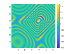
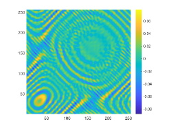
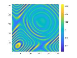
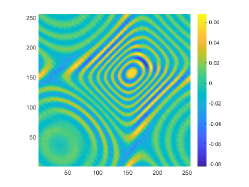
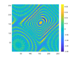
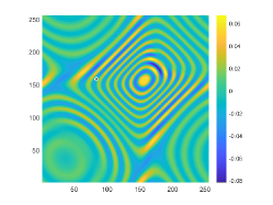
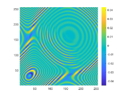
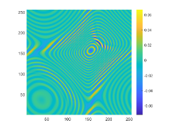
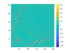
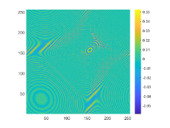
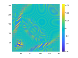
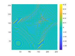
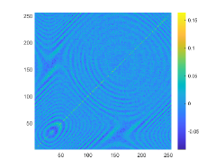
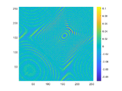
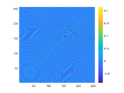
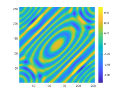
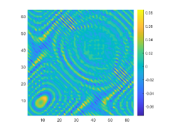
Figure 2. The imaginary parts of Cjmsubscript𝐶𝑗𝑚C_{jm} and Njmssubscriptsuperscript𝑁𝑠𝑗𝑚N^{s}_{jm} with ξ=0.4𝜉0.4\xi=0.4 and ξ=2𝜉2\xi=2 in the case of L=64𝐿64L=64 for the kite (Top) and the peanut (Bottom). The first column displays the imaginary parts of Cjmsubscript𝐶𝑗𝑚C_{jm} with ξ=0.4𝜉0.4\xi=0.4, the second column displays the imaginary parts of Cjmsubscript𝐶𝑗𝑚C_{jm} with ξ=2𝜉2\xi=2 and the third column displays the imaginary parts of Njmssubscriptsuperscript𝑁𝑠𝑗𝑚N^{s}_{jm}.
Refer to caption
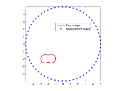
(a) Exact shape
Refer to caption
(b) ξ=0.4𝜉0.4\xi=0.4
Refer to caption
(c) ξ=2𝜉2\xi=2
Refer to caption
(d) Exact shape
Refer to caption
(e) ξ=0.4𝜉0.4\xi=0.4
Refer to caption
(f) ξ=2𝜉2\xi=2
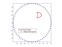
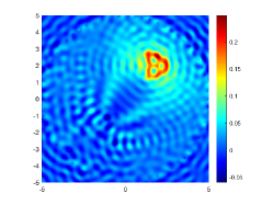
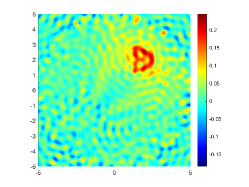
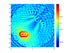
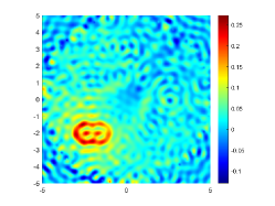
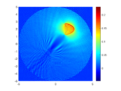
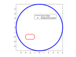
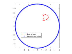
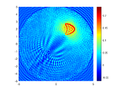
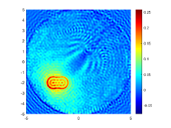
Figure 3. Recoveries of D𝐷\partial D by DCM with ξ=0.4𝜉0.4\xi=0.4 and ξ=2𝜉2\xi=2 in the case of L=64𝐿64L=64 for the kite (Top) and the peanut (Bottom). The first column shows the exact boundary D𝐷\partial D and L=64𝐿64L=64 measurement points, the second column shows the reconstructed D𝐷\partial D with ξ=0.4𝜉0.4\xi=0.4 and the third column shows the reconstructed D𝐷\partial D with ξ=2𝜉2\xi=2.
Refer to caption
(a) Im(Cjm),ξ=0.4Imsubscript𝐶𝑗𝑚𝜉0.4\mathrm{Im}(C_{jm}),\xi=0.4
Refer to caption
(b) Im(Cjm),ξ=2Imsubscript𝐶𝑗𝑚𝜉2\mathrm{Im}(C_{jm}),\xi=2
Refer to caption
(c) Im(Njms)Imsuperscriptsubscript𝑁𝑗𝑚𝑠\mathrm{Im}(N_{jm}^{s})
Refer to caption
(d) Im(Cjm),ξ=0.4Imsubscript𝐶𝑗𝑚𝜉0.4\mathrm{Im}(C_{jm}),\xi=0.4
Refer to caption
(e) Im(Cjm),ξ=2Imsubscript𝐶𝑗𝑚𝜉2\mathrm{Im}(C_{jm}),\xi=2
Refer to caption
(f) Im(Njms)Imsuperscriptsubscript𝑁𝑗𝑚𝑠\mathrm{Im}(N_{jm}^{s})
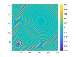
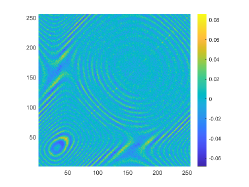
Figure 4. The imaginary parts of Cjmsubscript𝐶𝑗𝑚C_{jm} and Njmssubscriptsuperscript𝑁𝑠𝑗𝑚N^{s}_{jm} with ξ=0.4𝜉0.4\xi=0.4 and ξ=2𝜉2\xi=2 in the case of L=256𝐿256L=256 for the kite (Top) and the peanut (Bottom). The first column displays the imaginary parts of Cjmsubscript𝐶𝑗𝑚C_{jm} with ξ=0.4𝜉0.4\xi=0.4, the second column displays the imaginary parts of Cjmsubscript𝐶𝑗𝑚C_{jm} with ξ=2𝜉2\xi=2 and the third column displays the imaginary parts of Njmssubscriptsuperscript𝑁𝑠𝑗𝑚N^{s}_{jm}.
Refer to caption
(a) Exact shape
Refer to caption
(b) ξ=0.4𝜉0.4\xi=0.4
Refer to caption
(c) ξ=2𝜉2\xi=2
Refer to caption
(d) Exact shape
Refer to caption
(e) ξ=0.4𝜉0.4\xi=0.4
Refer to caption
(f) ξ=2𝜉2\xi=2
Figure 5. Recoveries of D𝐷\partial D by DCM with ξ=0.4𝜉0.4\xi=0.4 and ξ=2𝜉2\xi=2 in the case of L=256𝐿256L=256 for the kite (Top) and the peanut (Bottom). The first column shows the exact boundary D𝐷\partial D and L=256𝐿256L=256 measurement points, the second column shows the reconstructed D𝐷\partial D with ξ=0.4𝜉0.4\xi=0.4 and the third column shows the reconstructed D𝐷\partial D with ξ=2𝜉2\xi=2.

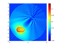
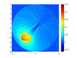
In this example, we are concerned with the imaging of the single obstacle. To this end, two different obstacles are considered, which are respectively kite-shaped and peanut-shaped. Their boundaries are respectively given by

D={(2+0.5(cosθ+0.65cos2θ0.65),2+0.75sinθ):θ[0,2π]}.𝐷conditional-set20.5𝜃0.652𝜃0.6520.75𝜃𝜃02𝜋\displaystyle\partial D=\Big{\{}\big{(}2+0.5(\cos\theta+0.65\cos 2\theta-0.65),2+0.75\sin\theta\big{)}:\theta\in[0,2\pi]\Big{\}}.

and

D={(2+cos2θ+0.25sin2θcosθ,2+cos2θ+0.25sin2θsinθ):θ[0,2π]}.𝐷conditional-set2superscript2𝜃0.25superscript2𝜃𝜃2superscript2𝜃0.25superscript2𝜃𝜃𝜃02𝜋\displaystyle\partial D=\Big{\{}\big{(}-2+\sqrt{\cos^{2}\theta+0.25\sin^{2}\theta}\cos\theta,-2+\sqrt{\cos^{2}\theta+0.25\sin^{2}\theta}\sin\theta\big{)}:\theta\in[0,2\pi]\Big{\}}.

This kite-shaped obstacle is also considered in [17], allowing us to compare our reconstructions with those of [17].

4.1.1. The influence of the perturbation ξ𝜉\xi and the number L𝐿L of incident random sources

We now consider to investigate the influence of the perturbation ξ𝜉\xi and the number L𝐿L of random point sources on the solution of the inverse problem by using noise-free data, i.e., δ=0𝛿0\delta=0. The wavenumber is k=2π𝑘2𝜋k=2\pi.

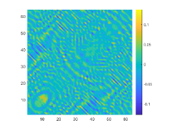
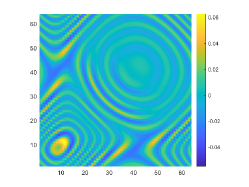
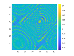
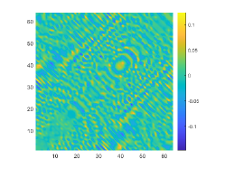
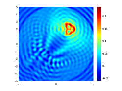
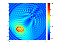
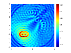
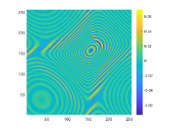
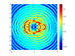
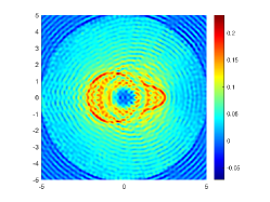
We first look at how ξ𝜉\xi affects the reconstruction. For this purpose, we set ξ=0.4𝜉0.4\xi=0.4 and ξ=2𝜉2\xi=2, respectively. Moreover, we choose L=64𝐿64L=64. The imaginary parts of the cross-correlations Cjmsubscript𝐶𝑗𝑚C_{jm} with ξ=0.4𝜉0.4\xi=0.4 and ξ=2𝜉2\xi=2 for the kite are shown in Fig. 2(a) and (b), and the imaginary parts of the cross-correlations Cjmsubscript𝐶𝑗𝑚C_{jm} for the peanut are shown in Fig. 2(d) and (e). The corresponding approximate imaginary parts of Njmssubscriptsuperscript𝑁𝑠𝑗𝑚N^{s}_{jm} for the kite and peanut are respectively presented in Fig. 2(c) and (f). Fig. 2 shows that larger ξ𝜉\xi will generate larger approximation error between Cjmsubscript𝐶𝑗𝑚C_{jm} and Njmssubscriptsuperscript𝑁𝑠𝑗𝑚N^{s}_{jm}. The boundary reconstructions of our proposed DCM with ξ=0.4𝜉0.4\xi=0.4 and ξ=2𝜉2\xi=2 are shown in Fig. 3. It is clear in Fig. 3 that, our proposed DCM can obtain satisfactory reconstructions. Moreover, Fig. 3 indicates that as ξ𝜉\xi increases, the reconstruction of the location and shape will be accordingly distorted. This is reasonable because Cjmsubscript𝐶𝑗𝑚C_{jm} is the discrete approximation of Njmssubscriptsuperscript𝑁𝑠𝑗𝑚N^{s}_{jm} and the corresponding discrete error that will affect the reconstruction deeply relies on ξ𝜉\xi. It is worth noticing that our proposed DCM also works well for ξ=2𝜉2\xi=2 although Theorem 3.1 does not cover ξ1/2𝜉12\xi\geq 1/2.

It is expected by Theorem 3.1 that the inversion quality can be improved by more incident random sources. Hence, the total number L𝐿L is increased to be L=256𝐿256L=256. In the case of L=256𝐿256L=256, the imaginary parts of the corresponding cross-correlations Cjmsubscript𝐶𝑗𝑚C_{jm} with ξ=0.4𝜉0.4\xi=0.4 and ξ=2𝜉2\xi=2 for the kite can be seen in Fig. 4(a) and (b), and the imaginary parts of the cross-correlations Cjmsubscript𝐶𝑗𝑚C_{jm} for the peanut are shown Fig. 4(d) and (e). The approximate imaginary parts of Njmssubscriptsuperscript𝑁𝑠𝑗𝑚N^{s}_{jm} are shown in Fig. 4(c) and (f). We find from Fig. 4 that compared with the results in Fig. 2, the discrete error between Cjmsubscript𝐶𝑗𝑚C_{jm} and Njmssubscriptsuperscript𝑁𝑠𝑗𝑚N^{s}_{jm} is significantly reduced particularly for ξ=0.4𝜉0.4\xi=0.4. The reconstructions of the kite and peanut for L=256𝐿256L=256 are presented in Fig. 5. As expected, in Fig. 5 the reconstructions are improved when L𝐿L increases. This confirms Theorem 3.1. Therefore, to meet the required conditions of Theorem 3.1 and maintain the high-quality inversion, we set ξ=0.4𝜉0.4\xi=0.4 and L=256𝐿256L=256 in all the following examples. Moreover, the phenomenon in this experiment also holds for the noisy case.

4.1.2. The influence of the wavenumber k𝑘k
Refer to caption
(a) Im(Cjm),k=4πImsubscript𝐶𝑗𝑚𝑘4𝜋\mathrm{Im}(C_{jm}),k=4\pi
Refer to caption
(b) Im(Cjm),k=4πImsubscript𝐶𝑗𝑚𝑘4𝜋\mathrm{Im}(C_{jm}),k=4\pi
Refer to caption
(c) Im(Njms),k=4πImsuperscriptsubscript𝑁𝑗𝑚𝑠𝑘4𝜋\mathrm{Im}(N_{jm}^{s}),k=4\pi
Refer to caption
(d) Im(Njms),k=4πImsuperscriptsubscript𝑁𝑗𝑚𝑠𝑘4𝜋\mathrm{Im}(N_{jm}^{s}),k=4\pi
Refer to caption
(e) Im(Cjm),k=8πImsubscript𝐶𝑗𝑚𝑘8𝜋\mathrm{Im}(C_{jm}),k=8\pi
Refer to caption
(f) Im(Cjm),k=8πImsubscript𝐶𝑗𝑚𝑘8𝜋\mathrm{Im}(C_{jm}),k=8\pi
Refer to caption
(g) Im(Njms),k=8πImsuperscriptsubscript𝑁𝑗𝑚𝑠𝑘8𝜋\mathrm{Im}(N_{jm}^{s}),k=8\pi
Refer to caption
(h) Im(Njms),k=8πImsuperscriptsubscript𝑁𝑗𝑚𝑠𝑘8𝜋\mathrm{Im}(N_{jm}^{s}),k=8\pi
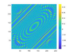
Figure 6. The imaginary parts of Cjmsubscript𝐶𝑗𝑚C_{jm} and Njmssubscriptsuperscript𝑁𝑠𝑗𝑚N^{s}_{jm} with k=4π𝑘4𝜋k=4\pi and k=8π𝑘8𝜋k=8\pi for the kite (Left) and the peanut (Right). The first row displays the imaginary parts of Cjmsubscript𝐶𝑗𝑚C_{jm} with k=4π𝑘4𝜋k=4\pi, the second row displays the imaginary parts of Njmssubscriptsuperscript𝑁𝑠𝑗𝑚N^{s}_{jm} with k=4π𝑘4𝜋k=4\pi, the third row displays the imaginary parts of Cjmsubscript𝐶𝑗𝑚C_{jm} with k=8π𝑘8𝜋k=8\pi and the fourth row displays the imaginary parts of Njmssubscriptsuperscript𝑁𝑠𝑗𝑚N^{s}_{jm} with k=8π𝑘8𝜋k=8\pi.
Refer to caption
(a) Exact shape
Refer to caption
(b) k=4π𝑘4𝜋k=4\pi
Refer to caption
(c) k=8π𝑘8𝜋k=8\pi
Refer to caption
(d) Exact shape
Refer to caption
(e) k=4π𝑘4𝜋k=4\pi
Refer to caption
(f) k=8π𝑘8𝜋k=8\pi
Figure 7. Recoveries of D𝐷\partial D by DCM with k=4π𝑘4𝜋k=4\pi and k=8π𝑘8𝜋k=8\pi for the kite (Top) and the peanut (Bottom). The first column shows the exact boundary D𝐷\partial D and L=256𝐿256L=256 measurement points, the second column shows the reconstructed D𝐷\partial D with k=4π𝑘4𝜋k=4\pi and the third column shows the reconstructed D𝐷\partial D with k=8π𝑘8𝜋k=8\pi.

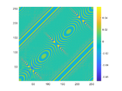
The obstacle reconstructions with different k𝑘k are considered by using noise-free data, i.e., δ=0𝛿0\delta=0. We set k=4π𝑘4𝜋k=4\pi and k=8π𝑘8𝜋k=8\pi. The imaginary parts of the cross-correlations Cjmsubscript𝐶𝑗𝑚C_{jm} with k=4π𝑘4𝜋k=4\pi and k=8π𝑘8𝜋k=8\pi for the kite-shaped obstacle and the peanut-shaped obstacle are plotted in the first and third rows of Fig. 6. The approximate active imaginary parts of Njmssubscriptsuperscript𝑁𝑠𝑗𝑚N^{s}_{jm} are shown in the second and fourth rows of Fig. 6, respectively. The results of Fig. 6 also confirm the formula (3.9) that describes the relationship between Cjmsubscript𝐶𝑗𝑚C_{jm} and Njmssubscriptsuperscript𝑁𝑠𝑗𝑚N^{s}_{jm}. We present the boundary reconstructions of D𝐷\partial D with k=4π𝑘4𝜋k=4\pi and k=8π𝑘8𝜋k=8\pi for the kite and the peanut in Fig. 7.

It is noted in Fig. 7 that with the increase of the wavenumber k𝑘k, more detailed geometrical information can be attained, which can significantly improve inversion quality. This phenomenon occurs mainly because as the wavenumber k𝑘k increases, smaller probe wavelength can be used and kS|ψ(x^,τ)|2dx^𝑘subscript𝑆superscriptsuperscript𝜓^𝑥𝜏2differential-d^𝑥k\int_{S}|\psi^{\infty}(\hat{x},\tau)|^{2}\mathrm{d}\hat{x} in Theorem 3.1 is accordingly increased. Furthermore, compared with the reconstructions of the kite-shaped scatterer in [17] for high wavenumber, reconstructions obtained by our DCM are more accurate.

4.1.3. The influence of the noise level δ𝛿\delta
Refer to caption
(a) Im(Cjmδ),δ=0.2Imsubscriptsuperscript𝐶𝛿𝑗𝑚𝛿0.2\mathrm{Im}(C^{\delta}_{jm}),\delta=0.2
Refer to caption
(b) Im(Cjmδ),δ=0.4Imsubscriptsuperscript𝐶𝛿𝑗𝑚𝛿0.4\mathrm{Im}(C^{\delta}_{jm}),\delta=0.4
Refer to caption
(c) Im(Njms)Imsuperscriptsubscript𝑁𝑗𝑚𝑠\mathrm{Im}(N_{jm}^{s})
Refer to caption
(d) Im(Cjmδ),δ=0.2Imsubscriptsuperscript𝐶𝛿𝑗𝑚𝛿0.2\mathrm{Im}(C^{\delta}_{jm}),\delta=0.2
Refer to caption
(e) Im(Cjmδ),δ=0.4Imsubscriptsuperscript𝐶𝛿𝑗𝑚𝛿0.4\mathrm{Im}(C^{\delta}_{jm}),\delta=0.4
Refer to caption
(f) Im(Njms)Imsuperscriptsubscript𝑁𝑗𝑚𝑠\mathrm{Im}(N_{jm}^{s})
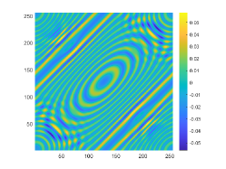
Figure 8. The imaginary parts of Cjmδsubscriptsuperscript𝐶𝛿𝑗𝑚C^{\delta}_{jm} and Njmssubscriptsuperscript𝑁𝑠𝑗𝑚N^{s}_{jm} with δ=0.2𝛿0.2\delta=0.2 and δ=0.4𝛿0.4\delta=0.4 for the kite (Top) and the peanut (Bottom). The first column displays the imaginary parts of Cjmδsubscriptsuperscript𝐶𝛿𝑗𝑚C^{\delta}_{jm} with δ=0.2𝛿0.2\delta=0.2, the second column displays the imaginary parts of Cjmδsubscriptsuperscript𝐶𝛿𝑗𝑚C^{\delta}_{jm} with δ=0.4𝛿0.4\delta=0.4 and the third column displays the imaginary parts of Njmssubscriptsuperscript𝑁𝑠𝑗𝑚N^{s}_{jm}.
Refer to caption
(a) Exact shape
Refer to caption
(b) δ=0.2𝛿0.2\delta=0.2
Refer to caption
(c) δ=0.4𝛿0.4\delta=0.4
Refer to caption
(d) Exact shape
Refer to caption
(e) δ=0.2𝛿0.2\delta=0.2
Refer to caption
(f) δ=0.4𝛿0.4\delta=0.4
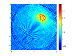
Figure 9. Recoveries of D𝐷\partial D by DCM with δ=0.2𝛿0.2\delta=0.2 and δ=0.4𝛿0.4\delta=0.4 for the kite (Top) and the peanut (Bottom). The first column shows the exact boundary D𝐷\partial D and L=256𝐿256L=256 measurement points, the second column shows the reconstructed D𝐷\partial D with δ=0.2𝛿0.2\delta=0.2 and the third column shows the reconstructed D𝐷\partial D with δ=0.4𝛿0.4\delta=0.4.

The above two experiments are only conducted in the noise-free case. However, the observation data is typically perturbed by the noise due to the limitation of many practical scenarios. Hence, in this example, we shall consider the influence of the noise level δ𝛿\delta. To do so, we set δ=0.2𝛿0.2\delta=0.2 and δ=0.4𝛿0.4\delta=0.4, respectively. The wavenumber is k=4π𝑘4𝜋k=4\pi. We present the imaginary parts of the cross-correlations Cjmδsubscriptsuperscript𝐶𝛿𝑗𝑚C^{\delta}_{jm} with δ=0.2𝛿0.2\delta=0.2 and δ=0.4𝛿0.4\delta=0.4 for the kite-shaped obstacle in Fig. 8(a) and (b), and the imaginary parts of the cross-correlations for the peanut-shaped obstacle are shown in Fig. 8(d) and (e). The approximate active imaginary parts of Njmssubscriptsuperscript𝑁𝑠𝑗𝑚N^{s}_{jm} for the kite and the peanut can be seen in Fig. 8(c) and (f). Clearly, the error between Cjmδsubscriptsuperscript𝐶𝛿𝑗𝑚C^{\delta}_{jm} and Njmssubscriptsuperscript𝑁𝑠𝑗𝑚N^{s}_{jm} will become larger when the noise level δ𝛿\delta increases, which is reasonable since in the noisy case the error between Cjmδsubscriptsuperscript𝐶𝛿𝑗𝑚C^{\delta}_{jm} and Njmssubscriptsuperscript𝑁𝑠𝑗𝑚N^{s}_{jm} is generated by not only the quadrature error of the trapezoidal rule approximation but also the added noise. The recovery results of the boundary D𝐷\partial D are shown in Fig. 9, from which we clearly observe that our proposed DCM can obtain satisfactory reconstructions even for the case of δ=0.4𝛿0.4\delta=0.4. In fact, this is expected since Theorem 3.2 has theoretically indicated that our proposed DCM is extremely stable with respect to the added noise.
4.2. Example 2: Multiple obstacles case

In this example, we aim to investigate the performance of our DCM in the more complicated case of multiple obstacles. The noise level is chosen as δ=0.2𝛿0.2\delta=0.2.

4.2.1. Tow obstacles close to each other
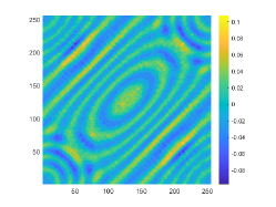
Refer to caption
(a) Im(Cjmδ),k=2πImsubscriptsuperscript𝐶𝛿𝑗𝑚𝑘2𝜋\mathrm{Im}(C^{\delta}_{jm}),k=2\pi
Refer to caption
(b) Im(Njms),k=2πImsuperscriptsubscript𝑁𝑗𝑚𝑠𝑘2𝜋\mathrm{Im}(N_{jm}^{s}),k=2\pi
Refer to caption
(c) Im(Cjmδ),k=4πImsubscriptsuperscript𝐶𝛿𝑗𝑚𝑘4𝜋\mathrm{Im}(C^{\delta}_{jm}),k=4\pi
Refer to caption
(d) Im(Njms),k=4πImsuperscriptsubscript𝑁𝑗𝑚𝑠𝑘4𝜋\mathrm{Im}(N_{jm}^{s}),k=4\pi
Figure 10. The imaginary parts of Cjmδsubscriptsuperscript𝐶𝛿𝑗𝑚C^{\delta}_{jm} and Njmssubscriptsuperscript𝑁𝑠𝑗𝑚N^{s}_{jm} with k=2π𝑘2𝜋k=2\pi (Top) and k=4π𝑘4𝜋k=4\pi (Bottom) for the resolution limit case. The first column displays the imaginary parts of Cjmδsubscriptsuperscript𝐶𝛿𝑗𝑚C^{\delta}_{jm} with k=2π𝑘2𝜋k=2\pi and k=4π𝑘4𝜋k=4\pi, and the second column displays the imaginary parts of Njmssubscriptsuperscript𝑁𝑠𝑗𝑚N^{s}_{jm} with k=2π𝑘2𝜋k=2\pi and k=4π𝑘4𝜋k=4\pi.
Refer to caption
(a) Exact shape
Refer to caption
(b) k=2π𝑘2𝜋k=2\pi
Refer to caption
(c) k=4π𝑘4𝜋k=4\pi
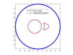
Figure 11. Recoveries of D𝐷\partial D by DCM with k=2π𝑘2𝜋k=2\pi and k=4π𝑘4𝜋k=4\pi for the resolution limit. The first column shows the exact boundary D𝐷\partial D and L=256𝐿256L=256 measurement points, the second column shows the reconstructed D𝐷\partial D with k=2π𝑘2𝜋k=2\pi and the third column shows the reconstructed D𝐷\partial D with k=4π𝑘4𝜋k=4\pi.

We consider the imaging of two scatterers close to each other in this experiment. Thus, the considered obstacle D𝐷D is the union of two bounded simply connected domains, i.e., D=D1D2𝐷subscript𝐷1subscript𝐷2D=D_{1}\bigcup D_{2}. Moreover, these two scatterers are disjoint. Here, the parameterized forms of D1subscript𝐷1D_{1} and D2subscript𝐷2D_{2} are given by

D1={(2+0.5(cosθ+0.65cos2θ0.65),0.75sinθ):θ[0,2π]},subscript𝐷1conditional-set20.5𝜃0.652𝜃0.650.75𝜃𝜃02𝜋\displaystyle\partial D_{1}=\bigg{\{}(2+0.5(\cos\theta+0.65\cos 2\theta-0.65),0.75\sin\theta):\theta\in[0,2\pi]\bigg{\}},

and

D2={(0.7+1.5cosθ,1.5sinθ):θ[0,2π]}.subscript𝐷2conditional-set0.71.5𝜃1.5𝜃𝜃02𝜋\displaystyle\partial D_{2}=\bigg{\{}(-0.7+1.5\cos\theta,1.5\sin\theta):\theta\in[0,2\pi]\bigg{\}}.

Indeed, these two obstacles are very close to each other and the distance two obstacles is about 0.5. Therefore, we set k=2π𝑘2𝜋k=2\pi and k=4π𝑘4𝜋k=4\pi for imaging D𝐷D and the corresponding probe wavelength defined by 2πk2𝜋𝑘\frac{2\pi}{k} are respectively 1 and 0.5. The imaginary parts of the cross-correlations Cjmδsubscriptsuperscript𝐶𝛿𝑗𝑚C^{\delta}_{jm} for k=2π𝑘2𝜋k=2\pi and k=4π𝑘4𝜋k=4\pi are plotted in Fig. 10(a) and (c), respectively. The approximate active imaginary parts of Njmssubscriptsuperscript𝑁𝑠𝑗𝑚N^{s}_{jm} are respectively shown in Fig. 10(b) and (d). Fig. 10 indicates that even for two obstacles close to each other, the approximation relationship between Cjmδsubscriptsuperscript𝐶𝛿𝑗𝑚C^{\delta}_{jm} and Njmssubscriptsuperscript𝑁𝑠𝑗𝑚N^{s}_{jm} also holds. The reconstructions of D𝐷\partial D in the resolution limit case with k=2π𝑘2𝜋k=2\pi and k=4π𝑘4𝜋k=4\pi are presented in Fig. 11. In the k=2π𝑘2𝜋k=2\pi case, the gap between these two obstacles is about half a wavelength. However, we unfortunately find from Fig. 11(b) that for the wavenumber k=2π𝑘2𝜋k=2\pi the considered two obstacles can not be well distinguished. When the wavenumber is increased to k=4π𝑘4𝜋k=4\pi, the gap between two obstacles can be clearly depicted.

4.2.2. Multiscale

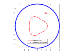
We now turn our attention to the case of multiscale. To this end, we set k=4π𝑘4𝜋k=4\pi and k=8π𝑘8𝜋k=8\pi, respectively. Furthermore, the considered obstacle D=D1D2𝐷subscript𝐷1subscript𝐷2D=D_{1}\bigcup D_{2} is the union of a big pear-shaped obstacle D1subscript𝐷1D_{1} located at (0,0)00(0,0) and a small disk centered at (2,3)23(2,3) with the radius 0.2. Here, the parameterized forms of D1subscript𝐷1D_{1} and D2subscript𝐷2D_{2} are given by

D1={(2+0.3cos3θ)(cosθ,sinθ):θ[0,2π]},subscript𝐷1conditional-set20.33𝜃𝜃𝜃𝜃02𝜋\displaystyle\partial D_{1}=\bigg{\{}(2+0.3\cos 3\theta)(\cos\theta,\sin\theta):\theta\in[0,2\pi]\bigg{\}},

and

D2={(2+0.2cosθ,3+0.2sinθ):θ[0,2π]}.subscript𝐷2conditional-set20.2𝜃30.2𝜃𝜃02𝜋\displaystyle\partial D_{2}=\bigg{\{}(2+0.2\cos\theta,3+0.2\sin\theta):\theta\in[0,2\pi]\bigg{\}}.

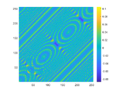
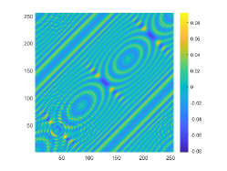
The imaginary parts of the cross-correlations Cjmδsubscriptsuperscript𝐶𝛿𝑗𝑚C^{\delta}_{jm} for k=4π𝑘4𝜋k=4\pi and k=8π𝑘8𝜋k=8\pi in the multiscale case are plotted in Fig. 12(a) and (c), respectively. The approximate active imaginary parts of Njmssubscriptsuperscript𝑁𝑠𝑗𝑚N^{s}_{jm} are respectively shown in Fig. 12(b) and (d). From Fig. 12 we find that Cjmδsubscriptsuperscript𝐶𝛿𝑗𝑚C^{\delta}_{jm} is also the discrete approximation of Njmssubscriptsuperscript𝑁𝑠𝑗𝑚N^{s}_{jm} for the multiscale case. We show the reconstructions of D𝐷\partial D in the multiscale case with k=4π𝑘4𝜋k=4\pi and k=8π𝑘8𝜋k=8\pi in Fig. 13. It is clear in Fig. 13 that our proposed DCM is capable of recovering both the big and small obstacles.
Refer to caption
(a) Im(Cjmδ),k=4πImsubscriptsuperscript𝐶𝛿𝑗𝑚𝑘4𝜋\mathrm{Im}(C^{\delta}_{jm}),k=4\pi
Refer to caption
(b) Im(Njms),k=4πImsuperscriptsubscript𝑁𝑗𝑚𝑠𝑘4𝜋\mathrm{Im}(N_{jm}^{s}),k=4\pi
Refer to caption
(c) Im(Cjmδ),k=8πImsubscriptsuperscript𝐶𝛿𝑗𝑚𝑘8𝜋\mathrm{Im}(C^{\delta}_{jm}),k=8\pi
Refer to caption
(d) Im(Njms),k=8πImsuperscriptsubscript𝑁𝑗𝑚𝑠𝑘8𝜋\mathrm{Im}(N_{jm}^{s}),k=8\pi
Figure 12. The imaginary parts of Cjmδsubscriptsuperscript𝐶𝛿𝑗𝑚C^{\delta}_{jm} and Njmssubscriptsuperscript𝑁𝑠𝑗𝑚N^{s}_{jm} with k=4π𝑘4𝜋k=4\pi (Top) and k=8π𝑘8𝜋k=8\pi (Bottom) for the multiscale case. The first column displays the imaginary parts of Cjmδsubscriptsuperscript𝐶𝛿𝑗𝑚C^{\delta}_{jm} with k=4π𝑘4𝜋k=4\pi and k=8π𝑘8𝜋k=8\pi, and the second column displays the imaginary parts of Njmssubscriptsuperscript𝑁𝑠𝑗𝑚N^{s}_{jm} with k=4π𝑘4𝜋k=4\pi and k=8π𝑘8𝜋k=8\pi.
Refer to caption
(a) Exact shape
Refer to caption
(b) k=4π𝑘4𝜋k=4\pi
Refer to caption
(c) k=8π𝑘8𝜋k=8\pi
Figure 13. Recoveries of D𝐷\partial D by DCM with k=4π𝑘4𝜋k=4\pi and k=8π𝑘8𝜋k=8\pi for the multiscale case. The first column shows the exact boundary D𝐷\partial D and L=256𝐿256L=256 measurement points, the second column shows the reconstructed D𝐷\partial D with k=4π𝑘4𝜋k=4\pi and the third column shows the reconstructed D𝐷\partial D with k=8π𝑘8𝜋k=8\pi.

5. Summary

This work focuses on developing a direct imaging method, known as the doubly cross-correlating method (DCM), for recovering a sound-soft obstacle in a passive imaging system. The fundamental challenges in this passive inverse scattering problem is the randomness of the incident sources, making direct solutions based on collected total fields inefficient. DCM addresses this by providing a cross-correlation between passive observations that can be linked to the active inverse scattering problem using the Helmholtz-Kirchhoff identity, thereby removing the randomness provided by incident point sources. This cross-correlation is then utilized to create an imaging function to visualize the obstacle. Because it relies merely on matrix multiplication, DCM is computationally efficient and simple to implement. Furthermore, the methodology presented in this work can be extended to sound-hard cases, penetrable cases, and even three-dimensional scenarios, which will be investigated in the future.

References

  • [1] H. Ammari, G. Bao, and J. Fleming. An inverse source problem for maxwell’s equations in magnetoencephalography. SIAM Journal on Applied Mathematics, 62(4):1369–1382, 2002.
  • [2] A. P. Austin and L. N. Trefethen. Trigonometric interpolation and quadrature in perturbed points. SIAM Journal on Numerical Analysis, 55(5):2113–2122, 2017.
  • [3] G. Bao, J. Lin, and S. M. Mefire. Numerical reconstruction of electromagnetic inclusions in three dimensions. SIAM Journal on Imaging Sciences, 7(1):558–577, 2014.
  • [4] B. Borden. Mathematical problems in radar inverse scattering. Inverse Problems, 18(1):R1, 2001.
  • [5] C. Borges and L. Greengard. Inverse obstacle scattering in two dimensions with multiple frequency data and multiple angles of incidence. SIAM Journal on Imaging Sciences, 8(1):280–298, 2015.
  • [6] S. N. Chandler-Wilde, I. G. Graham, S. Langdon, and M. Linder. Condition number estimates for combined potential boundary integral operators in acoustic scattering. The Journal of Integral Equations and Applications, 21(2):229–279, 2009.
  • [7] Y. Chang and Y. Guo. Simultaneous recovery of an obstacle and its excitation sources from near-field scattering data. Electronic Research Archive, 30:1296–1321, 2022.
  • [8] Y. Chang, Y. Guo, H. Liu, and D. Zhang. Recovering source location, polarization, and shape of obstacle from elastic scattering data. Journal of Computational Physics, 489(15):112289, 2023.
  • [9] J. Chen, Z. Chen, and G. Huang. Reverse time migration for extended obstacles: acoustic waves. Inverse Problems, 29(8):085005, 2013.
  • [10] J. Chen, Z. Chen, and G. Huang. Reverse time migration for extended obstacles: electromagnetic waves. Inverse Problems, 29(8):085006, 2013.
  • [11] Z. Chen, S. Fang, and G. Huang. A direct imaging method for the half-space inverse scattering problem with phaseless data. Inverse Probl. Imaging, 11:901–916, 2017.
  • [12] Z. Chen and G. Huang. Reverse time migration for reconstructing extended obstacles in the half space. Inverse Problems, 31(5):055007, 2015.
  • [13] Z. Chen and G. Huang. A direct imaging method for electromagnetic scattering data without phase information. SIAM Journal on Imaging Sciences, 9(3):1273–1297, 2016.
  • [14] Z. Chen and G. Huang. Phaseless imaging by reverse time migration: acoustic waves. Numerical Mathematics: Theory, Methods and Applications, 10(1):1–21, 2017.
  • [15] Z. Chen and S. Zhou. A direct imaging method for half-space inverse elastic scattering problems. Inverse Problems, 35(7):075004, 2019.
  • [16] D. Colton and R. Kress. Inverse Acoustic and Electromagnetic Scattering Theory. Springer, New York, 2019.
  • [17] J. Garnier, H. Haddar, and H. Montanelli. The linear sampling method for random sources. SIAM Journal on Imaging Sciences, 16(3):1572–1593, 2023.
  • [18] J. Garnier, H. Haddar, and H. Montanelli. The linear sampling method for data generated by small random scatterers. arXiv preprint arXiv:2403.19482, 2024.
  • [19] J. Garnier and G. Papanicolaou. Passive imaging with ambient noise. Cambridge University Press, Cambridge, 2016.
  • [20] Y. Guo, F. Ma, and D. Zhang. An optimization method for acoustic inverse obstacle scattering problems with multiple incident waves. Inverse Problems in Science and Engineering, 19(4):461–484, 2011.
  • [21] X. Ji, X. Liu, and B. Zhang. Target reconstruction with a reference point scatterer using phaseless far field patterns. SIAM Journal on Imaging Sciences, 12(1):372–391, 2019.
  • [22] A. Kirsch and N. Grinberg. The factorization method for inverse problems, volume 36. OUP Oxford, 2007.
  • [23] A. Kirsch and R. Kress. A numerical method for an inverse scattering problem. Journal of Inverse and Ill-Posed Problems, 3:279–289, 1987.
  • [24] A. Kirsch and R. Kress. An optimization method in inverse acoustic scattering. Boundary Elements IX, vol. 3: Fluid flow and potential applications, ed C.A. Brebbia et al, Berlin, Springer,, pages 3–18, 1987.
  • [25] A. Kirsch and X. Liu. A modification of the factorization method for the classical acoustic inverse scattering problems. Inverse Problems, 30(3):035013, 2014.
  • [26] R. Kress. Newtons method for inverse obstacle scattering meets the method of least squares. Inverse Problems, 19(6):91–104, 2003.
  • [27] R. Kress and W. Rundell. A quasi-newton method in inverse obstacle scattering. Inverse Problems, 10(5):1145–1157, 1994.
  • [28] P. Kuchment. The radon transform and medical imaging. CBMS-NSF Regional Conference Series in Applied Mathematics, Society for Industrial and Applied Mathematics, 2014.
  • [29] J. Li. Reverse time migration for inverse obstacle scattering with a generalized impedance boundary condition. Applicable Analysis, 101(1):48–62, 2022.
  • [30] J. Li, H. Wu, and J. Yang. Reverse time migration for inverse acoustic scattering by locally rough surfaces. arXiv preprint arXiv:2211.11325, 2022.
  • [31] J. Li and J. Yang. Simultaneous recovery of a locally rough interface and the embedded obstacle with the reverse time migration. arXiv preprint arXiv:2211.11329, 2022.
  • [32] J. Li and J. Zou. A direct sampling method for inverse scattering using far-field data. Inverse Problems and Imaging, 7(1):757–775, 2013.
  • [33] X. Liu. A novel sampling method for multiple multiscale targets from scattering amplitudes at a fixed frequency. Inverse Problems, 33(8):085011, 2017.
  • [34] X. Liu, S. Meng, and B. Zhang. Modified sampling method with near field measurements. SIAM Journal on Applied Mathematics, 82(1):244–266, 2022.
  • [35] W. McLean. Strongly elliptic systems and boundary integral equations. Cambridge university press, 2000.
  • [36] R. Potthast. A study on orthogonality sampling. Inverse Problems, 26(7):074015, 2010.
  • [37] P. Serranho. A hybrid method for inverse scattering for shape and impedance. Inverse Problems, 22(2):663–680, 2006.
  • [38] J. Yang, B. Zhang, and H. Zhang. Reconstruction of complex obstacles with generalized impedance boundary conditions from far-field data. SIAM Journal on Applied Mathematics, 74(1):106–124, 2014.
  • [39] Y. Yin and L. Yan. Bayesian model error method for the passive inverse scattering problem. Inverse Problems, 40(6):065005, 2024.
  • [40] B. Zhang and H. Zhang. An approximate factorization method for inverse acoustic scattering with phaseless total-field data. SIAM Journal on Applied Mathematics, 80(5):2271–2298, 2020.
  • [41] D. Zhang, Y. Chang, and Y. Guo. Jointly determining the point sources and obstacle from cauchy data. Inverse Problems, 40(1):015014, 2023.
  • [42] D. Zhang, Y. Guo, Y. Wang, and Y. Chang. Co-inversion of a scattering cavity and its internal sources: uniqueness, decoupling and imaging. Inverse Problems, 39(6):065004, 2023.