A Novel 3D Mapping Representation and its Applications
Abstract
The analysis of mapping relationships and distortions in multidimensional data poses a significant challenge in contemporary research. While Beltrami coefficients offer a precise description of distortions in two-dimensional mappings, current tools lack this capability in the context of three-dimensional space. This paper presents a novel approach: a 3D quasiconformal representation that captures the local dilation of 3D mappings, along with a reconstruction algorithm that establishes a connection between this representation and the corresponding mapping. Experimental results showcase the algorithm’s effectiveness in mapping reconstruction, keyframe interpolation, and mapping compression. These features bear a resemblance to the 2D Linear Beltrami Solver technique. The work presented in this paper offers a promising solution for the precise analysis and adjustment of distortions in 3D data and mappings.
Keywords Quasiconformal mapping, Beltrami coefficient, 3D quasiconformal representation, 3D Linear Beltrami Solver, Keyframe interpolation, 3D mapping compression
1 Introduction
In modern scientific research, one of the main motivations is to process the vast amount of information encountered by human beings. This information includes 1D, 2D, and 3D data, which we encounter daily. Acoustic algorithms have been developed to process 1D information such as voice, while image data captured by cameras, rendered in games, and used in medical scenarios, such as X-ray images, are examples of 2D data. In mathematics, we consider surfaces on a 3D object as 2D and typically parameterize them on the 2D plane for further processing. 3D information includes MRI from brain, CT scans for chest, etc.
When analyzing relationships between pairs or groups of objects, we often use mappings to represent these relationships. However, when working with mappings, it’s important to be mindful of the distortion that can arise from numerical implementations. In the 2D case, Beltrami coefficients, which are based on the Beltrami equation, can be used to measure the distortion of 2D mappings effectively. By controlling or analyzing the Beltrami coefficients of mappings, we can perform registration or shape analysis. However, this approach only works for 2D space. Unfortunately, we currently lack such an effective tool to describe distortion in 3D space precisely.
For a long time, we had no efficient way to reconstruct mappings from Beltrami coefficients. Obtaining Beltrami coefficients from mappings is straightforward, but the inverse direction is not explicitly defined in the Beltrami equation. However, the Linear Beltrami Solver (LBS) [1] has tackled this problem by providing an effective link between Beltrami coefficients and mappings. LBS has been successful in the field of mapping distortion adjustment, enabling the adjustment of distortion in both forward and backward directions. Various algorithms based on LBS have been proposed to solve challenging problems such as efficient parameterization, image registration, segmentation, retargeting, deturbulence, Teichmuller mapping, and harmonic Beltrami signature. Recently, some learning-based methods have been developed based on LBS, leveraging prior knowledge from data and the topological preservation advantages of LBS to effectively address challenging tasks and outperform conventional methods in various aspects.
However, LBS is theoretically based on the Beltrami’s equation, which can only provides a relationship between Beltrami coefficients and mappings in 2D space. when dealing with distortions in 3D space, LBS and its related efficient algorithms cannot be generalized for use in three dimensions. Unlike in 2D space, there is no quasiconformal representation similar to Beltrami coefficients in 3D space, nor is there an equation that relates this representation to its corresponding mapping.
In this paper, we propose a 3D quasiconformal representation that can effectively describe the local dilation of a 3D mapping and an algorithm similar to LBS, connecting this representation and its corresponding mapping. We also propose a keyframe interpolation algorithm and a 3D mapping compression algorithm based on the proposed 3D quasiconformal representation and the reconstruction algorithm. Experimental results show the effectiveness of this algorithm.
2 Contributions
The main contributions of this paper are outlined as follows.
-
1.
We propose an effective 3D quasiconformal representation to describe the local dilation of 3D mappings.
-
2.
We derive a partial differential equation that connects the proposed 3D quasiconformal representation and its corresponding mapping. Similar to LBS, this PDE can be discretized into a linear system, and boundary conditions and landmarks can be imposed easily.
-
3.
We further show that under our discretization scheme, the resulting linear system is symmetric positive definite, meaning that the linear system can be solved efficiently using the conjugate gradient method.
-
4.
Based on the above algorithm, we propose an algorithm for 3D keyframe interpolation in the film and animation industry.
-
5.
Based on the above algorithm, we propose a 3D mapping compression algorithm for 3D unstructured mesh.
3 Related works
The computational method of conformal mapping [2, 3] has proven to be highly beneficial in the field of computer graphics. After the groundbreaking study by Gu et al. [4], there has been significant progress in using the conformal geometry framework for surface processing tasks. The work of Zayer, Rossl, and Seidel [5] already contains implicit generalizations of these ideas. Lui and his coauthors proposed the quasi-conformal extension of the surface registration framework, which includes the map compression [6] and the Linear Beltrami Solver (LBS) introduced in [1]. This solver has been used to develop fast spherical and disk conformal parameterization techniques [7, 8], as well as various registration algorithms for different applications [9, 10, 11, 12, 13, 14, 15, 16, 17, 18, 19, 20, 21, 22, 23, 24]. Additionally, LBS has been utilized in various segmentation algorithms for different applications [25, 26, 27, 28]. Besides, it has also been applied to shape analysis [29, 30, 31, 32, 33, 34]. Learning-based methods based on LBS [35, 36] were also proposed to perform topology-preserving registration in the 2D space. However, due to the limitation of the quasiconformal theory the LBS is based on, these useful techniques have not been generalized to process 3D data.
Some efforts have been made to apply the quasiconformal theory to process data with higher dimensions. In [37], a generalized conformality distortion is first defined to measure the dilatation of a n-dimensional quasiconformal map, after which optimization algorithms are proposed to obtain landmark-matching transformation. Based on this quantity, [38] proposes a general framework for various n-dimensional mapping problems. [39] proposes an n-dimensional measure that is consistent with the classical 2D Beltrami coefficient in terms of the relationship between the magnitude of the quantity and the determinant of the mapping. Although these quantities are effective in measuring and controlling the distortion of mappings, the generalized conformality distortion cannot be used to reconstruct 3D mappings, as they do not contain the complete information (dilation in three orthogonal directions) of mapping, and the lack of information makes obtaining the mappings from the defined quantities impossible. In other words, they are not equivalent quantities to the Beltrami coefficient in the higher dimension.
4 Mathematical background
In the following sections, we will introduce the Mathematical background for this paper. It includes three parts, polar decomposition for decomposing rotation and dilation, quasiconformal mapping in the 2D space, and some observation related to matrix inverse.
4.1 Polar decomposition
In this paper, we focus solely on the left polar decomposition for real rectangular matrices. We begin by denoting the set of real matrices as . The left polar decomposition of a matrix is a factorization of the form , where the columns of the matrix form an orthonormal basis, and is a symmetric positive semi-definite matrix. Specifically, .
To better understand this definition, we first note that is a symmetric semi-definite matrix. By applying the eigenvalue decomposition to this matrix, we have
where is an orthogonal matrix because is symmetric, therefore we also have . The diagonal matrix contains the eigenvalues of . denotes the matrix whose diagonal entries are the square root of the corresponding entries in . Those diagonal entries are the singular values of . Thus, we have .
Therefore, any linear transformation from to is a composition of a rotation/reflection and a dilation.
4.2 2D Quasiconformal maps and Beltrami coefficients
A surface with a conformal structure is known as a Riemann surface. Given two Riemann surfaces and , a map is conformal if it preserves the surface metric up to a multiplicative factor called the conformal factor. Quasiconformal maps are a generalization of conformal maps that are orientation-preserving diffeomorphisms between Riemann surfaces with bounded conformal distortion, meaning that their first-order approximation maps small circles to small ellipses of bounded eccentricity (as shown in Figure 1).
Mathematically, a map is quasiconformal if it satisfies the Beltrami equation
for some complex valued functions with called the Beltrami coefficient. In particular, is conformal around a small neighborhood of a point if and only if , that is
This equation shows that can be considered as a map composed of a translation that maps to , followed by a stretch map , which is postcomposed by a multiplication of a conformal map . Among these terms, causes to map small circles to small ellipses, and controls the stretching effect of . By denoting and , where , and representing in a matrix form, we have
| (1) |
One can check that the eigenvalues for this matrix are and . The eigenvectors for this matrix are and respectively. It is worth noting that the two eigenvectors are orthogonal to each other. The distortion or dilation can be measured by . Thus the Beltrami coefficient gives us important information about the properties of a map.
4.3 An observation related to matrix inverse
In addition, we notice some interesting results related to matrix inverse, which facilitate the derivation in the following sections.
Generally, for any invertible matrix , we have
Representing the row vectors of as , , and , and the column vectors as , , and , we have
| (2) | ||||
| (3) |
5 3D mapping representation
In this section, we will provide a detailed description of our proposed 3D mapping representation for diffeomorphisms. We call it a “representation” because it includes all the information needed to reconstruct the corresponding mapping, which is a feature not present in many existing methods. Therefore we have a reconstruction method for the proposed representation.
The organization of this section is as follows. We begin by extending the Beltrami coefficients to 3D space. Since there is no Beltrami equation for 3D space, we refer to these extended coefficients as 3D quasiconformal representation. Next, we derive an elliptic partial differential equation that relates the mappings to their 3D quasiconformal representation. Finally, we discretize the equation to obtain a linear system. By solving this system with appropriate boundary conditions, we can reconstruct mappings from their representation. Then we summarize the proposed representation and reconstruction algorithm using pseudo code. Experimental results for mapping reconstruction are provided at the end of this section to demonstrate the performance of our algorithm.
5.1 3D quasiconformal representation
Let and be oriented, simply connected open subsets of . Suppose we have a diffeomorphism . denotes the Jacobian matrix of at a point in . Since is diffeomorphic, it is invertible. As a result, the Jacobian determinant is always positive for every point in .
Let be the diagonal matrix containing the singular values of , where by convention, we require that . By polar decomposition, we have
| (4) | ||||
where is a rotation matrix, because the determinant of and are greater than 0, implying that . are the eigenvalues of representing the dilation information, and is an orthogonal matrix containing eigenvectors for dilation.
Recall that in 2D space, the Beltrami coefficient encodes the two dilation and , together with their corresponding directions and , which are orthogonal to each other. Now in 3D space, we have three dilations , , and , together with their corresponding directions represented by the column vectors of , which are also orthogonal to each other, as is symmetric. Therefore, similar to the Beltrami coefficient, encodes the dilation information of the 3D mapping .
Furthermore, it is possible to represent the matrix by Euler angles. To do so, we require that the column vectors of form an orthonormal basis, and . However, the is not necessarily positive, meaning that may not be a rotation matrix. This can be fixed by randomly multiplying a column of by to get a matrix . This modification ensures , indicating that is a rotation matrix, while at the same time, the matrix will not be changed. To see this, the matrix can be reorganized as , where are the column vectors of . Let , then . Thus reversing the direction of makes no change to . This also holds for and .
As is known, a rotation matrix can be written in the following form:
| (5) | ||||
Then we obtain the Euler angles by
| (6) | ||||
In conclusion, we have the following two equivalent ways to define 3D quasiconformal representation for diffeomorphism:
-
1.
The upper triangular part of the matrix . is a symmetric positive definite matrix, therefore the upper triangular part can encode the information of the matrix;
-
2.
The eigenvalues and the Euler angles . The Euler angles encode the information of the eigenvectors, therefore they include the equivalent information of .
Note that both representations include 6 numbers for each point in the domain. The first representation facilitates various computational operations, as the angles are not involved during the computation, while the second representation provides a much clearer geometric meaning. Since the two representations are equivalent and can be easily converted to each other, we will use only the first representation, i.e., the upper triangular part of , in the following sections without further mention.
5.2 The PDE in the continuous case
Recall the assumption that is a diffeomorphism, implying is invertible. Right multiplying by on both side of the above equation, we have
| (9) |
where is the adjugate matrix of . According to the observation mentioned in Equation 2, has the form
| (10) |
where , and are the columns of .
Moving the terms before the matrix C on the right-hand side of Equation 9 to the left, we have
| (11) |
Let be a matrix defined as
| (12) |
We can rewrite Equation 11 in the following form
| (13) |
For , we have
| (14) |
since results in zero vector. This also holds for and .
Therefore, we compute divergence on both sides of Equation 13 to get the following equations
| (15) | ||||
Furthermore, we define as the 3D generalized Laplacian operator.
5.3 Discretisation and implementation
In the 2D case, we typically triangularize the domain to obtain finite elements and then define a piecewise linear function on that domain to approximate a smooth mapping. In the 3D case, we need to define the piecewise linear function on tetrahedrons serving as the elements.
Consider a 3D simply connected domain discretized into a tetrahedral mesh containing vertices and tetrahedrons represented by the set of index sets . Also, the order of the vertices in a tetrahedron should satisfy a condition: the determinant of the matrix consisting of the three vectors , , and must be positive, or equivalently, .
In this setting, the mapping is piecewise linear.
To compute the 3D quasiconformal representation for , we need to compute at each point in . Since is piecewise linear, the Jacobian matrices at each point in the same tetrahedron are equal to each other, resulting in the same polar decomposition and 3D quasiconformal representation. Therefore, we simply need to compute the Jacobian matrices at each tetrahedron , denoted as , and use it to get . The linear function defined on each tetrahedron can be written as
| (16) |
We can then compute the polar decomposition of using Equations 4, which subsequently provides the 3D quasiconformal representation for .
To reconstruct the mapping , we need the matrix , which contains the 3D representation information. Once given the representation at a point , at can be computed according to Equation 12. As every point in shares the same dilation, is a piecewise-constant matrix-valued function, where takes a constant matrix value within each , which we denote as .
To construct the discrete version of Equations 15, we should first derive the discrete gradient operator. For a certain tetrahedron , let , where . Then we have the equation
| (17) |
where
| (18) |
Then moving the matrix to the right, we have
| (19) |
For simplicity, we index the values in by the form , where are the row and column of the indexed entry.
We define
| (20) |
Then we have the following result, from which we know that , , and compose the discrete gradient operator .
| (21) |
The remaining part is the divergence operator. We first look at the definition of divergence. In a connected domain , the divergence of a vector field F evaluated at a point is defined as
| (22) |
where denotes the volume of , is the boundary surface of , is the outward unit normal to , and is the flux of F across .
In the discrete case, a vertex is surrounded by a set of tetrahedrons . Considering that our goal is not to develop a discrete divergence operator that can give precise divergence at every vertex, but to solve Equations 15 to get , , and such that the divergence of these functions is approximately equal to 0, we propose to replace the divergence operator by computing the flux in the discrete setting. The flux of F evaluated at can be written as follows
| (23) |
here we use to denote the triangle opposite to , is the outward unit normal to the triangle , and represents the vector field defined on . In our setting, is a piecewise-constant vector field, where takes a constant vector value within each .
Considering that we shrink to whose corresponding vertices satisfy , , and . Then the flux
since in the discrete setting, , , and . Therefore, if we require , then
where , and therefore, as , . Although the above equation is not strictly equivalent to , it motivates us to approximate using .
To solve the problem, we need to rewrite Equation 23 into a computable form. The quantity in the summation of Equation 23 can be evaluated using the property introduced in Equation 3. By comparing with the matrix in Equation 3, we notice that the three row vectors of satisfy
where represents the volume of with respect to , and .
For vertex , the outward normal vector on is given by
We also know that . The geometric meaning of is shown in Figure 2.
Together, for the term in the summation of flux evaluated at the four vertices of , we have
Then the flux can be rewritten as
Denoting the three row vectors of as , then by substituting , , and into F, we have the following equations
| (24) | ||||
Note that in Equations 24, the components , , and are derived from the source mesh, i.e., and , which are not related to the unknowns , , and , and comes from the given 3D quasiconformal representation. Reorganizing Equations 24, we get three linear systems
| (25) |
In order to introduce boundary conditions, for the given boundary vertices for the function indexed by from to with the target value , we first define a vector , where is the “one-hot” vector that has 1 in the -th entry and zero in the remaining entries. Then a temporary vector can be computed, after which we set the -th entry of to correspondingly to get the vector . Similarly, for the function and , we can generate and .
We define an operation called “masking” as follows: for a given boundary vertex , we set the -th row and -th column of to zero, and the -th diagonal entry to 1.
We perform the masking operation to for all the boundary vertices to get the matrices , , and .
Then we have
| (26) |
and the mapping can then be reconstructed.
5.4 Analysis
In this section, we would like to show that the linear systems 26 are symmetric positive definite (SPD). Compared with triangular mesh encountered in the 2D cases, tetrahedral meshes possess more vertices, resulting in large linear systems that are hard to solve. But if the linear systems are SPD, then we can use efficient numerical methods, such as the conjugate gradient method, to solve it more efficiently.
We will divide this section into two parts, in which we show the symmetry of and the positive definiteness of the linear systems.
5.4.1 Symmetry of
In this section, we would like to show that the matrix in Equations 25 is symmetric. To see this, we may turn first to the incidence matrix of a tetrahedral mesh.
The incidence matrix of a tetrahedral mesh is a matrix that describes the connectivity between the vertices and the tetrahedrons in the mesh. Specifically, it captures which vertices are part of which tetrahedrons. In our setting, the incidence matrix is an matrix, where is the number of tetrahedrons and is the number of vertices. Each row corresponds to a tetrahedron, and each column corresponds to a vertex. If a vertex belongs to a tetrahedron, the corresponding entry in the matrix is set to ; otherwise, it is set to .
Suppose we have a discrete function defined on the vertices of the mesh. If we want to sum up the function values on the vertices of each tetrahedron, we can simply compute , which yields the desired results. If we want to compute the weighted sum, we can simply replace the entries by the weights, and then compute .
In our case, we want to construct a matrix that can compute the discrete gradient for each tetrahedron. Recall that we compute the gradient of over by taking the dot product . In the implementation, is a dimensional vector. To compute for all tetrahedrons, we first construct the incidence matrix for the mesh, and then replace the values in by the corresponding to get the matrix . Then we can compute the gradient over of all tetrahedrons by simply computing . Similarly, we can construct and with and to compute the gradient of over and .
Now we can construct a matrix, where -th row ( from to ) is replaced by the -th row of , -th row is replaced by the -th row of , and -th row is replaced by the -th row of . We denote this matrix as , as it serves as the discrete gradient operator. can be regarded as an block matrix, each block computes the gradient vector for the corresponding tetrahedron . Also, each block has only nonzero columns indexed by , the values of which are .
Then we can consider the matrix , which is a . For any discrete function defined on the tetrahedrons of the mesh, sums up the values on the tetrahedrons surrounding each vertex . Similarly, the weighted sum can be computed by first replacing the values in by the weights.
In our case, has a similar structure to . Suppose we have a discrete vector field defined on the tetrahedrons of the mesh, we can put the vectors into a dimensional vector according to the index of the tetrahedrons in . Then, computing is equivalent to computing .
Recall that our formula has a term. We can further define a block diagonal matrix , each diagonal block of which is , which is a matrix. Obviously, is SPD.
The last component is a block diagonal matrix , each diagonal block of which is . Since the 3D representation assigned to each tetrahedron corresponds to an SPD matrix, the eigenvalues of this matrix are all positive, and they compose the eigenvalues of , we know that is also SPD. Therefore, is SPD.
Together, we have . As is SPD, and and are the diagonal blocks of and respectively, we know that is SPD as well, and as a result, is a symmetric matrix. We denote as in the following section for simplicity. Also, since is SPD, there exists an invertible matrix such that .
5.4.2 Positive definiteness
In this section, we would like to show that , , and in the linear systems 26 are SPD. The proof of symmetry is trivial since the masking operation does not change the symmetry, but the proof of positive definiteness is not trivial, and we first prove some lemmas and propositions which facilitate the proof. For succinctness, in this section, we denote the number of vertices by (i.e., ).
Lemma 1.
, and the vector is the only basis vector in the null space of .
Proof.
Matrix computes the gradient of a discrete function on tetrahedrons. If for some vector , then by definition, the gradient of on every tetrahedron is zero, meaning that for some constant on each tetrahedron. Therefore, is the only basis vector in the null space of . This shows that is in the null space of .
Then we aim to prove the uniqueness. If there exists a nonzero vector such that , then is orthogonal to the row vectors of , or equivalently, , where C denotes the columns space. However, for any nonzero vector satisfying for any constant , we have nonzero vector , , indicating that . In other words, for any nonzero vector , there does not exist a nonzero vector such that . Therefore, the null space of is only span by .
Hence, . ∎
Lemma 2.
Any column (or row) vector in can be expressed as a linear combination of the rest column (or row) vectors.
Proof.
Matrix is symmetric and therefore diagonalizable. Let , where is an orthogonal matrix containing the eigenvectors as columns, and is a diagonal matrix with the eigenvalues. By Lemma 1, , indicating that one of its eigenvalues is zero, and the rest are non-zero. Without loss of generality, let the last diagonal entry in be 0, and the last column of be the vector . In this setting, the last row of is equal to .
Each column of can be expressed as a linear combination of the columns in , or equivalently, the first columns in , as the last eigenvalue is . The linear combination coefficients are stored in .
Let be the first columns of , then is the first rows of . Let be the entry in the last row of , then . Denote the column vectors in as for , then since is an orthogonal matrix, the column vectors are perpendicular to each other, and the length of each vector is , we have:
Randomly pick column vectors from to form the matrix . Then we have:
where is an identity matrix, and is a matrix full of 1s.
Let . Suppose is an eigenvalue of , then , or . We know that the eigenvalue of is on the eigenvector , and 0 on the other eigenvectors. Therefore, the eigenvalues of are on , and on the other eigenvectors. Hence:
Thus, with multiplicity , or with multiplicity , and:
which implies:
which indicates is full rank, and is also full rank. Therefore, any column vectors in form a basis in the -dimensional space, and the remaining vector can be expressed as a linear combination of the basis.
Let be the first columns of and let . Then by the above proof, we know that there exists an dimensional nonzero vector such that . Then we have .
In the left-hand side, is the -th column of , while in the right-hand side, is the matrix containing the remaining column vectors of . The equation means that the -th column vector of can be expressed as a linear combination of the remaining column vectors of , and the coefficients are stored in .
As the index can be randomly chosen, we prove the statement for column vectors. Since the matrix is symmetric, this property can be extended to the row vectors as well. ∎
We can set the -th row and -th column of to zero. With Lemma 2, we know that the rank of this matrix is still .
Also, we know that the vector lies in the null space of this matrix. By setting the -th diagonal entry to , we get a full rank matrix, which is denoted as .
Proposition 1.
is an SPD matrix.
Proof.
Setting the -th column in to zero, we get a new matrix denoted as . By the above definition, we have
where is an matrix whose -th diagonal entry is , and all other entries are zero. The matrix is the same matrix obtained by setting -th row and -th column of to , the rank of which is . Then we decompose any nonzero vector into and , where is the value in the -th entry of , and denotes the vector with the -th component removed.
Then, we have
Since and is full rank, . Together with the definition of , we know that its null space only includes and its row space contains the remaining components. Since contains the complementary components of , is nonzero if is nonzero. Otherwise, if is a zero vector, then is nonzero because is nonzero. Therefore, the two terms and cannot be zero at the same time. Then , which proves the statement. ∎
For any SPD matrix , we set the -th row and -th column of to be zero, and set the -th diagonal entry to , then we get a new matrix .
Proposition 2.
is also SPD.
Proof.
Since is an SPD matrix, it can be decomposed to where contains the eigenvalues, which are all positive.
Then, by setting the -th row of to , we get another matrix . Then we have
where is an matrix whose -th diagonal entry is , and all other entries are zero.
Then we decompose any nonzero vector into and , where is the value in the -th entry of , and denotes the vector with the -th component removed.
Then we have,
where . Since , . Apparently, we notice that the vector is the only basis in the null space of . Since contains the complementary components of , is nonzero if is nonzero. Otherwise, if is a zero vector, then is nonzero because is nonzero. Therefore, the two terms and cannot be zero at the same time. Then , which proves the statement. ∎
With the above Lemmas and Propositions, we can now show that
Theorem 1.
, , and in the linear systems 26 are SPD.
5.5 Pseudo-codes
This section provides a summary of the algorithms discussed in the previous sections by presenting the pseudo-codes for each method, as shown in Algorithm 1 and 2.
5.6 Experiments
This section presents experimental results demonstrating the effectiveness of our proposed 3D quasiconformal representation and reconstruction algorithm on 3D tetrahedral meshes. For each experiment, we first show the source and target meshes with the same number of vertices and connections, thereby forming a mapping. Then we show the reconstructed mapping from the 3D quasiconformal representation obtained from the given mapping. As we believe the proposed representation contains sufficient information about its corresponding mapping, we expect the reconstructed mapping to be as close to the mapping as possible, resulting in small reconstruction errors determined by the norm between the original mappings and the reconstructed mappings.
Also in the following experiments, we use the same boundary condition that
where .
Figures 3,4, and 5 show the reconstruction results for two bijective mappings, and the reconstruction errors are , , and , respectively. These small errors demonstrate that our approach is effective at reconstructing mappings using their 3D quasiconformal representations, yielding precise results for bijective mappings.

6 Applications
The above representation can be applied to 3D animation interpolation and mapping compression. In the following, we will introduce these two applications and show their experimental results.
6.1 3D keyframe interpolation
In the film and animation industry, animation is generally created by first designing two keyframes and then interpolating between them to get the intermediate frames.
In this section, we provide a novel keyframe interpolation method based on the proposed 3D representation, which takes the geometric information of the mapping into account.
Given two keyframes and , which are two triangular meshes with the same number of vertices and triangulation, our first step is to embed them into unit cubic domains and respectively.
Then we fill with vertices. This step is necessary because it can ensure that the resulting mapping can map to without folding. If the vertices are too sparse, there may not be enough freedom for the vertices to move while satisfying the constraint that the mapping should be diffeomorphic.
However, adding too many vertices to the domain should be avoided, as it can significantly increase the dimension of the linear system and slow down the solving process. Therefore, we propose first to use the Poisson disk sampling method [40] to randomly sample points in the domain evenly, and assign to each vertex a threshold, or in other words, a probability, based on the minimal distance between the vertex and the vertices on the triangular mesh. The formula used to generate the threshold is as follows
where denotes the minimal distance between the vertex and the vertices in , is the radius parameter of the Poisson disk sampling, and is the weight to control the sparsity. The first term is used to discard vertices that are too close to , and the second exponential term is used to discard those far away from . Then for each vertex , we assign it a random number in and decide whether to discard it by comparing the random number with .
is then tetrahedralized using tetgen [41]. We need to find a mapping such that:
-
1.
It is a diffeomorphism;
-
2.
It maps the vertices in to those in .
These can be achieved by using the efficient algorithm proposed in [38], which makes use of a generalized conformality term to control the distortion of the mapping.
With this mapping, we can map all the vertices in to diffeomorphically.
After that, we compute the representation for the mapping, which is a valued function. This function is piecewise constant on each tetrahedron.
Next, we can interpolate between the valued function for each tetrahedron and the upper triangular part of the identity matrix correspondingly.
Once we have the interpolated representation, we can reconstruct mappings for each frame with Equations 24 and boundary conditions.
In the following experiments, we show the interpolation results between human face meshes generated using 3D Morphable Model (3DMM) [42, 43], or registered human scans sampled from the FAUST dataset[44].
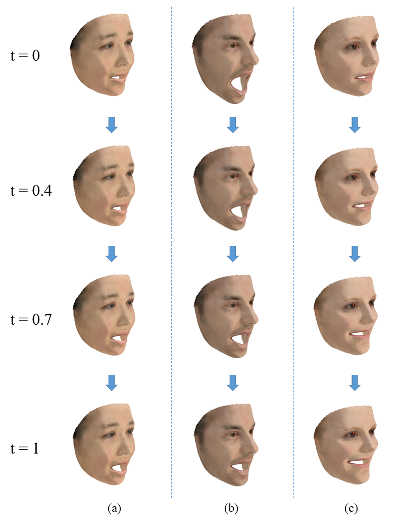
In Figure 6, we show three animation sequences generated using the proposed algorithm. The motion between the two keyframes of each sequence is mild, meaning that the distance between the 3D quasiconformal representations of the keyframes is comparatively small. Therefore, we expect it to work properly, and the experiment demonstrates that it works as expected.
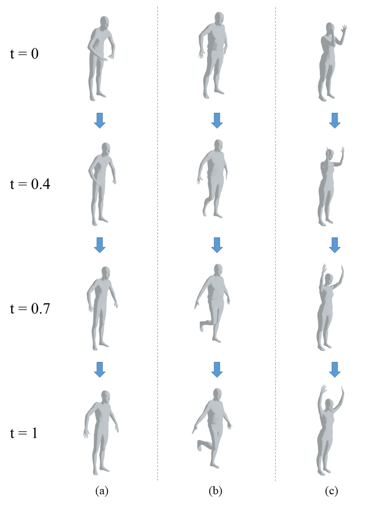
We also try to apply the algorithm to extreme cases, as shown in Figure 7, in which we show three animation sequences of human body motion. The scale of the motion between the two keyframes of each sequence is large, meaning that the distance between the 3D quasiconformal representations of the keyframes is large. The experiment demonstrates that our algorithm may work properly in some extreme cases.
6.2 3D mapping compression
Another application is to use the proposed 3D Representation to compress a 3D mapping.
Compared with 2D mapping, the storage requirement of 3D mappings is much higher. Nowadays, the prosperity of deep learning stimulates the need to create and store large datasets. With the development of the field of 3D animation, 3D data, which are generally much larger than 2D data, should be stored properly.
In this paper, we propose to store 3D mapping data using the proposed 3D representation. This representation has a good localized property, as the representation is defined on each tetrahedron and depicts the local distortion of the corresponding tetrahedron. In the following experiment, we will show that, compared with the coordinate function, our proposed representation has a better spectral property, which makes it suitable for mapping compression.
Our idea is similar to that in [1], in which the author compresses 2D mapping using discrete Fourier transform. However, when it comes to 3D mapping, the number of vertices increases dramatically. When the distribution of the vertices is very uneven, one may need a very dense regular grid to preserve the information of the original mesh precisely, which will boost the computation.
As we already have a mesh structure, it is a natural way to perform spectral analysis on the tetrahedral mesh directly. [45] introduces the idea of performing signal processing on a graph utilizing the graph Laplacian. In a discrete 2D surface with geometric information, signal processing can be applied with the Laplace-Beltrami operator, as introduced in [46, 47]. In the 3D case, the Laplace-Beltrami operator can also be computed using a 3D version cotangent formula [48, 49].
The 3D discrete Laplace-Beltrami operator is a matrix . Let be the subset of containing the tetrahedrons incident to an edge connecting and , then the weight of this edge is computed as
where is the edge connecting the other two vertices in , is the length of ; is the interior dihedral angle of edge connecting and .
Then the nonzero entries representing the edge connecting vertex and is
and diagonal element
for each vertex .
Then, by solving the generalized eigenvalue problem
| (27) |
where is the mass matrix whose diagonal , we obtain a series of eigenvalues satisfying , and their corresponding eigenvector satisfying for all generalized eigenvectors .
Let , then . Substituting it into Equation 27, we have , which is equivalent to . Note that is a symmetric matrix, and is its eigenvector, meaning that if . Thus, , meaning that the generalized eigenvectors of are -orthogonal to each other.
Therefore, we have for matrix whose column vectors are the generalized eigenvectors. Thus we have .
For any discrete function defined on the vertices of a tetrahedral mesh, the -inner product between and eigenvector is defined as
Then
as .
Therefore, we can project any function defined on a tetrahedral mesh to the spectral domain by computing -inner product with the generalized eigenvectors of the discrete Laplace-Beltrami operator. Also, the eigenvalues indicate the frequency of the eigenvectors. A larger eigenvalue corresponds to a higher frequency. With this property, we can perform low-pass or high-pass filtering to any function on the mesh.
In our case, suppose we have a pair of 3D meshes with the same number of vertices and triangulation. This couple forms a mapping. we would like to find a compressed representation for this mapping.
We first construct the discrete Laplace-Beltrami operator and the mass matrix for the source mesh.
Then we solve the generalized eigenvalue problem 27 with the constraint for all generalized eigenvectors to get the sorted eigenvalues and eigenvectors.
With the eigenvalues and eigenvectors, we can start to perform filtering to the 3D quasiconformal representation. A 3D representation is a piecewise linear vector-valued function defined on the tetrahedrons. We can treat this function as a combination of 6 scalar-valued functions, and perform filtering to the 6 functions separately.
For each of the 6 functions, we first interpolate it to the vertices of the mesh. Then we compute the -inner product for each eigenvector to get the spectrum. Based on the spectrum, one can select a threshold , and save and discard the rest. The smaller is, the more storage will be saved, but the reconstruction accuracy will be lower.
To reconstruct the function, one can read the saved spectral components , from the storage device. Then by computing
The vector-valued function representing the 3D representation can be reconstructed. One can reconstruct the mapping subsequently by solving the linear systems 24 with the reconstructed 3D representation.
There are two primary concerns regarding this 3D mapping compression scheme:
-
1.
Dimensionality Mismatch: The interpolated 3D representation is an valued function, whereas the coordinate function is an valued function. Consequently, to ensure that the storage requirements are comparable to those of storing the mapping directly, we must discard half of the spectral components. This process inevitably leads to a loss of information. However, our experimental results demonstrate that this operation is justified, as the significant information is primarily concentrated in the low-frequency region, making the loss due to the removal of high-frequency components relatively minor.
-
2.
Direct Compression of Coordinate Function: One might question why we do not compress the coordinate function directly. Our experiments reveal that attempting direct compression of the coordinate function yields poor results.
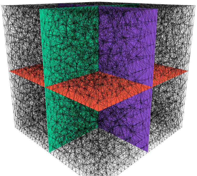
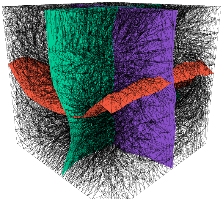
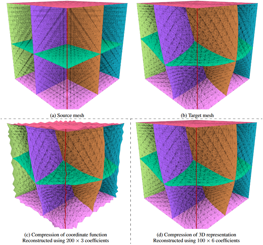
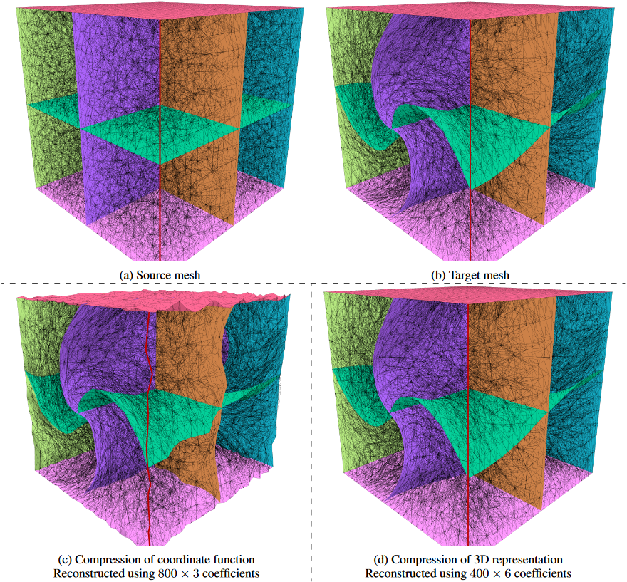
In the following experiments, we apply the above compression scheme to two 3D mappings. The experimental results are shown in Figures 8,9,10 and Figure 11,12,13 respectively.
Figures 8 and 11 show the two mappings and their compression results. (a) and (b) compose a mapping, (c) is the reconstructed result of compressing the coordinate function, and (d) is the reconstructed result of compressing the 3D representation. To illustrate the perturbation of the compressed mapping at the boundary, we have colored four of the outer surfaces of the tetrahedral mesh. Additionally, the edge where the two uncolored, transparent outer surfaces meet is highlighted in red.
In Figure 8, we see that the red edge in (c) deviates from its original position in (b). Also the four colored outer surfaces in (b) become turbulent if the mapping is compressed using the coordinate function. In comparison, the four outer surfaces and the red edge in (d) stay in their original position, as the proposed reconstruction algorithm allows us to introduce boundary conditions.
The deformation of the mapping shown in Figure 11 is much larger. Compared with the mesh in (b), apart from the deviation of the four colored outer surfaces and the red edge, we further notice that the three surfaces inside the cube are also distorted. In comparison, the shape of the three surfaces in (d) is well-preserved, which demonstrates the robustness of our algorithm.
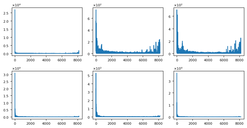
Figures 9 and 12 show the spectrum of the 3D representation for the two mappings. As the 3D representation is a valued function, we have one spectrum for each function respectively. From the two figures, we notice that most of the information is concentrated in the low-frequency domain, therefore, we can safely discard the coefficients corresponding to the high-frequency domain.
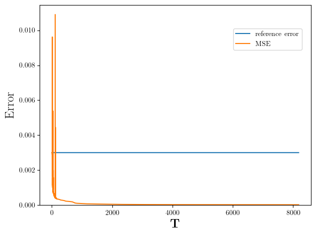
Figures 10 and 13 visualize the mean square error between the compressed mapping and the original one. The reference error is the mean square error between the source and target meshes. We see that as we discard more high-frequency coefficients, the error becomes larger. More importantly, we notice that the curves are flat except when the threshold is small, meaning that we can achieve a high compression ratio with the proposed mapping compression algorithm.
In conclusion, our proposed mapping compression algorithm shows the following superiority,
-
1.
It can be used to compress mapping defined on unstructured mesh;
-
2.
It allows the introduction of boundary conditions;
-
3.
It can compress mappings with a high compression ratio.
7 Conclusion
In this paper, we have proposed an effective 3D quasiconformal representation to describe the local dilation of 3D mappings. This representation, along with the associated reconstruction algorithm similar to Linear Beltrami Solver, allows us to process the mapping in the space of 3D quasiconformal representation.
We demonstrate the effectiveness of our proposed 3D quasiconformal representation and reconstruction algorithm. By reconstructing randomly generated discrete mappings defined on tetrahedral meshes with high precision, we demonstrate the correctness of the proposed reconstruction algorithm and the ability of the representation to encode distortion information.
We also show two applications enabled by the proposed 3D representation and the reconstruction algorithm. In the keyframe interpolation, we propose an alternative algorithm that enables the interpolation between keyframes in the space of 3D quasiconformal representation. The algorithm gives impressive results.
In mapping compression, we propose a compression algorithm for a mapping defined on unstructured mesh. It allows us to introduce boundary conditions so that we can control the domain easily. Also, it can achieve a high compression ratio for mappings with smooth deformation.
In future work, we plan to improve the computational efficiency of our algorithm and extend it to handle more complex deformations. We also aim to explore more applications where our technique could prove useful, including 3D image registration and image segmentation.
In summary, we have introduced an effective tool that, for the first time, fills the gap of describing and manipulating distortions in 3D space. The potential applications of our work are far-reaching, and we hope this newfound capability will prove invaluable for research involving 3D shapes and information.
References
- [1] L. M. Lui, K. C. Lam, T. W. Wong, and X. Gu, “Texture map and video compression using beltrami representation,” SIAM Journal on Imaging Sciences, vol. 6, no. 4, pp. 1880–1902, 2013.
- [2] M. Desbrun, M. Meyer, and P. Alliez, “Intrinsic parameterizations of surface meshes,” in Computer graphics forum, vol. 21. Wiley Online Library, 2002, pp. 209–218.
- [3] B. Lévy, S. Petitjean, N. Ray, and J. Maillot, “Least squares conformal maps for automatic texture atlas generation,” ACM transactions on graphics (TOG), vol. 21, no. 3, pp. 362–371, 2002.
- [4] X. Gu, Y. Wang, T. F. Chan, P. M. Thompson, and S.-T. Yau, “Genus zero surface conformal mapping and its application to brain surface mapping,” IEEE transactions on medical imaging, vol. 23, no. 8, pp. 949–958, 2004.
- [5] R. Zayer, C. Rossl, and H.-P. Seidel, “Discrete tensorial quasi-harmonic maps,” in International Conference on Shape Modeling and Applications 2005 (SMI’05). IEEE, 2005, pp. 276–285.
- [6] L. M. Lui, T. W. Wong, P. Thompson, T. Chan, X. Gu, and S.-T. Yau, “Compression of surface registrations using beltrami coefficients,” in 2010 IEEE Computer Society Conference on Computer Vision and Pattern Recognition. IEEE, 2010, pp. 2839–2846.
- [7] P. T. Choi, K. C. Lam, and L. M. Lui, “Flash: Fast landmark aligned spherical harmonic parameterization for genus-0 closed brain surfaces,” SIAM Journal on Imaging Sciences, vol. 8, no. 1, pp. 67–94, 2015.
- [8] P. T. Choi and L. M. Lui, “Fast disk conformal parameterization of simply-connected open surfaces,” Journal of Scientific Computing, vol. 65, pp. 1065–1090, 2015.
- [9] K. Chen, L. M. Lui, and J. Modersitzki, “Image and surface registration,” in Handbook of Numerical Analysis. Elsevier, 2019, vol. 20, pp. 579–611.
- [10] K. C. Lam, X. Gu, and L. M. Lui, “Genus-one surface registration via teichmüller extremal mapping,” in International Conference on Medical Image Computing and Computer-Assisted Intervention. Springer, 2014, pp. 25–32.
- [11] ——, “Landmark constrained genus-one surface teichmüller map applied to surface registration in medical imaging,” Medical image analysis, vol. 25, no. 1, pp. 45–55, 2015.
- [12] K. C. Lam and L. M. Lui, “Landmark-and intensity-based registration with large deformations via quasi-conformal maps,” SIAM Journal on Imaging Sciences, vol. 7, no. 4, pp. 2364–2392, 2014.
- [13] ——, “Quasi-conformal hybrid multi-modality image registration and its application to medical image fusion,” in International Symposium on Visual Computing. Springer, 2015, pp. 809–818.
- [14] L. M. Lui, K. C. Lam, S.-T. Yau, and X. Gu, “Teichmuller mapping (t-map) and its applications to landmark matching registration,” SIAM Journal on Imaging Sciences, vol. 7, no. 1, pp. 391–426, 2014.
- [15] L. M. Lui and C. Wen, “Geometric registration of high-genus surfaces,” SIAM Journal on Imaging Sciences, vol. 7, no. 1, pp. 337–365, 2014.
- [16] L. M. Lui, T. W. Wong, P. Thompson, T. Chan, X. Gu, and S.-T. Yau, “Shape-based diffeomorphic registration on hippocampal surfaces using beltrami holomorphic flow,” in International Conference on Medical Image Computing and Computer-Assisted Intervention. Springer, 2010, pp. 323–330.
- [17] L. M. Lui, T. W. Wong, W. Zeng, X. Gu, P. M. Thompson, T. F. Chan, and S.-T. Yau, “Optimization of surface registrations using beltrami holomorphic flow,” Journal of scientific computing, vol. 50, no. 3, pp. 557–585, 2012.
- [18] D. Qiu and L. M. Lui, “Inconsistent surface registration via optimization of mapping distortions,” Journal of Scientific Computing, vol. 83, no. 3, pp. 1–31, 2020.
- [19] C. Wen, D. Wang, L. Shi, W. C. Chu, J. C. Cheng, and L. M. Lui, “Landmark constrained registration of high-genus surfaces applied to vestibular system morphometry,” Computerized Medical Imaging and Graphics, vol. 44, pp. 1–12, 2015.
- [20] C. P. Yung, G. P. Choi, K. Chen, and L. M. Lui, “Efficient feature-based image registration by mapping sparsified surfaces,” Journal of Visual Communication and Image Representation, vol. 55, pp. 561–571, 2018.
- [21] W. Zeng, L. Ming Lui, and X. Gu, “Surface registration by optimization in constrained diffeomorphism space,” in Proceedings of the IEEE Conference on Computer Vision and Pattern Recognition, 2014, pp. 4169–4176.
- [22] D. Zhang, A. Theljani, and K. Chen, “On a new diffeomorphic multi-modality image registration model and its convergent gauss-newton solver,” Journal of Mathematical Research with Applications, vol. 39, no. 6, pp. 633–656, 2019.
- [23] M. Zhang, F. Li, X. Wang, Z. Wu, S.-Q. Xin, L.-M. Lui, L. Shi, D. Wang, and Y. He, “Automatic registration of vestibular systems with exact landmark correspondence,” Graphical models, vol. 76, no. 5, pp. 532–541, 2014.
- [24] D. Zhang and K. Chen, “A novel diffeomorphic model for image registration and its algorithm,” Journal of Mathematical Imaging and Vision, vol. 60, no. 8, pp. 1261–1283, 2018.
- [25] H.-L. Chan, S. Yan, L.-M. Lui, and X.-C. Tai, “Topology-preserving image segmentation by beltrami representation of shapes,” Journal of Mathematical Imaging and Vision, vol. 60, no. 3, pp. 401–421, 2018.
- [26] C. Y. Siu, H. L. Chan, and R. L. Ming Lui, “Image segmentation with partial convexity shape prior using discrete conformality structures,” SIAM Journal on Imaging Sciences, vol. 13, no. 4, pp. 2105–2139, 2020.
- [27] D. Zhang, X. cheng Tai, and L. M. Lui, “Topology- and convexity-preserving image segmentation based on image registration,” Applied Mathematical Modelling, vol. 100, p. 218, 2021.
- [28] D. Zhang and L. M. Lui, “Topology-preserving 3d image segmentation based on hyperelastic regularization,” Journal of Scientific Computing, vol. 87, no. 3, pp. 1–33, 2021.
- [29] H. L. Chan, H. Li, and L. M. Lui, “Quasi-conformal statistical shape analysis of hippocampal surfaces for alzheimer’s disease analysis,” Neurocomputing, vol. 175, pp. 177–187, 2016. [Online]. Available: https://www.sciencedirect.com/science/article/pii/S0925231215015064
- [30] H.-L. Chan, H.-M. Yuen, C.-T. Au, K. C.-C. Chan, A. M. Li, and L.-M. Lui, “Quasi-conformal geometry based local deformation analysis of lateral cephalogram for childhood osa classification,” arXiv preprint arXiv:2006.11408, 2020.
- [31] G. P. Choi, H. L. Chan, R. Yong, S. Ranjitkar, A. Brook, G. Townsend, K. Chen, and L. M. Lui, “Tooth morphometry using quasi-conformal theory,” Pattern Recognition, vol. 99, p. 107064, 2020.
- [32] G. P. Choi, D. Qiu, and L. M. Lui, “Shape analysis via inconsistent surface registration,” Proceedings of the Royal Society A, vol. 476, no. 2242, p. 20200147, 2020.
- [33] L. M. Lui, W. Zeng, S.-T. Yau, and X. Gu, “Shape analysis of planar multiply-connected objects using conformal welding,” IEEE transactions on pattern analysis and machine intelligence, vol. 36, no. 7, pp. 1384–1401, 2013.
- [34] T. W. Meng, G. P.-T. Choi, and L. M. Lui, “Tempo: Feature-endowed teichmuller extremal mappings of point clouds,” SIAM Journal on Imaging Sciences, vol. 9, no. 4, pp. 1922–1962, 2016.
- [35] Q. Chen, Z. Li, and L. M. Lui, “A deep learning framework for diffeomorphic mapping problems via quasi-conformal geometry applied to imaging,” arXiv preprint arXiv:2110.10580, 2021.
- [36] Y. Guo, Q. Chen, G. P. Choi, and L. M. Lui, “Automatic landmark detection and registration of brain cortical surfaces via quasi-conformal geometry and convolutional neural networks,” Computers in Biology and Medicine, p. 107185, 2023.
- [37] Y. T. Lee, K. C. Lam, and L. M. Lui, “Landmark-matching transformation with large deformation via n-dimensional quasi-conformal maps,” Journal of Scientific Computing, vol. 67, pp. 926–954, 2016.
- [38] D. Zhang, G. P. Choi, J. Zhang, and L. M. Lui, “A unifying framework for n-dimensional quasi-conformal mappings,” SIAM Journal on Imaging Sciences, vol. 15, no. 2, pp. 960–988, 2022.
- [39] C. Huang, K. Chen, M. Huang, D. Kong, and J. Yuan, “Topology-preserving image registration with novel multi-dimensional beltrami regularization,” Applied Mathematical Modelling, vol. 125, pp. 539–556, 2024.
- [40] R. L. Cook, “Stochastic sampling in computer graphics,” ACM Transactions on Graphics (TOG), vol. 5, no. 1, pp. 51–72, 1986.
- [41] S. Hang, “Tetgen, a delaunay-based quality tetrahedral mesh generator,” ACM Trans. Math. Softw, vol. 41, no. 2, p. 11, 2015.
- [42] V. Blanz and T. Vetter, “A morphable model for the synthesis of 3d faces,” in Proceedings of the 26th Annual Conference on Computer Graphics and Interactive Techniques, ser. SIGGRAPH ’99. USA: ACM Press/Addison-Wesley Publishing Co., 1999, p. 187–194. [Online]. Available: https://doi.org/10.1145/311535.311556
- [43] P. Paysan, R. Knothe, B. Amberg, S. Romdhani, and T. Vetter, “A 3d face model for pose and illumination invariant face recognition,” in 2009 sixth IEEE international conference on advanced video and signal based surveillance. Ieee, 2009, pp. 296–301.
- [44] F. Bogo, J. Romero, M. Loper, and M. J. Black, “Faust: Dataset and evaluation for 3d mesh registration,” in Proceedings of the IEEE conference on computer vision and pattern recognition, 2014, pp. 3794–3801.
- [45] D. I. Shuman, S. K. Narang, P. Frossard, A. Ortega, and P. Vandergheynst, “The emerging field of signal processing on graphs: Extending high-dimensional data analysis to networks and other irregular domains,” IEEE signal processing magazine, vol. 30, no. 3, pp. 83–98, 2013.
- [46] R. M. Rustamov et al., “Laplace-beltrami eigenfunctions for deformation invariant shape representation,” in Symposium on geometry processing, vol. 257, 2007, pp. 225–233.
- [47] K. Crane, “Discrete differential geometry: An applied introduction,” Notices of the AMS, Communication, vol. 1153, 2018.
- [48] ——, “The n-dimensional cotangent formula,” Online note. URL: https://www. cs. cmu. edu/~ kmcrane/Projects/Other/nDCotanFormula. pdf, pp. 11–32, 2019.
- [49] X. Gu, Y. Wang, and S.-T. Yau, “Volumetric Harmonic Map,” Communications in Information & Systems, vol. 3, no. 3, pp. 191 – 202, 2003.