A note on parallel preconditioning for the all-at-once solution of Riesz fractional diffusion equations

The governing Riesz fractional diffusion equations ¹¹1Here it is worth noting that if the Riesz fractional derivative is replaced with the fractional Laplacian, we can just follow the work in [50] for the spatial discretization of one- or two-dimensional model problem and our proposed numerical techniques in the next sections are easy and simple to be adapted for such an extension. of the anomalous diffusion process can be written as

where $u(x,t)$ may represent, for example, a solute concentration, and constant $\kappa_{\gamma}>0$ the diffusion coefficient. This equations is a superdiffusive model largely used in fluid flow analysis, financial modelling and other applications. The Riesz fractional derivative $\partial^{\gamma}u(x,t)/\partial|x|^{\gamma}$ is defined by [51]

in which ${}_{a}D^{\gamma}_{x}$ and ${}_{x}D^{\gamma}_{b}$ are the left and right Riemann-Liouville fractional derivatives of order $\gamma\in(1,2)$ given, respectively, by [5]

and

As $\gamma\rightarrow 2$, it notes that Eq. (2.1) degenerates into the classical diffusion equation [51].

Next, we focus on the numerical solution of Eq. (2.1). We consider a rectangle $\bar{Q}_{T}=\{(x,t):~{}a\leq x\leq b,~{}0\leq t\leq T\}$ discretized on the mesh $\varpi_{h\tau}=\varpi_{h}\times\varpi$, where $\varpi_{h}=\{x_{i}=a+ih,~{}i=0,1,\cdots,N;~{}h=(b-a)/N\}$, and $\varpi_{\tau}=\{t_{k}=k\tau,~{}j=0,1,\cdots,M;~{}\tau=T/M\}$. We denote by $v=\{v_{i}~{}|~{}0\leq i\leq N\}$ any grid function.

A considerable amount of work has been devoted in the past years to the development of fast methods for the approximation of the Riesz and Riemann-Liouville (R-L) fractional derivatives, such as the first-order accurate shifted Grünwald approximation [3, 51] and the second-order accurate weighted-shifted Grünwald difference (WSGD) approximation [9, 52]. Due to the relationship between the two kinds of fractional derivatives, all the numerical schemes proposed for the R-L fractional derivatives can be easily adapted to approximate the Riesz fractional derivative. Although the solution approach described in this work can accomodate any spatial discretized method, we choose the so-called fractional centred difference formula [8] of the Riesz fractional derivatives for clarity.

For any function $u(x)\in L^{1}(\mathbb{R})$, we denote

where the $\gamma$-dependent weight coefficient is defined as

As noted in [8], $\omega^{(\gamma)}_{\ell}=\mathcal{O}(\ell^{-1-\gamma})$ and the fractional centred difference formula $\Delta^{\gamma}_{h}u(x)$ exists for any $u(x)\in L^{1}(\mathbb{R})$. Some properties of the coefficient $\omega^{(\gamma)}_{\ell}$ and the operator $\Delta^{\gamma}_{h}u(x)$ are presented in the following lemmas.

At this stage, let $u(x,t)\in\mathcal{C}^{4,3}_{x,t}([a,b]\times[0,T])$ be a solution to the problem (2.1) and consider Eq. (2.1) at the set of grid points $(x,t)=(x_{i},t_{k})\in\bar{Q}_{T}$ with $i=1,2,\cdots,N-1,~{}k=1,\cdots,M$. The first-order time derivative at the point $t=t_{k}$ is approximated by the second-order backward difference formula, i.e.,

then we define $U^{k}_{i}=u(x_{i},t_{k})$ and $f^{k}_{i}=f(x_{i},t_{k})$ to obtain

where $\{R^{k}_{i}\}$ are small and satisfy the inequality

Note that we cannot omit the small term in the derivation of a two-level difference scheme that is not selfstarting from Eq. (2.7) due to the unknown information of $u(x_{i},t_{1})$. One of the most popular strategies to compute the first time step solution $u^{1}_{i}$ is to use a first-order backward Euler scheme (which is only used once). This yields the following implicit difference scheme [37, 10] for Eq. (2.1):

where

In order to implement the proposed scheme, here we define ${\bm{u}}^{k}=[u(x_{1},t_{k}),u(x_{2},t_{k}),\cdots,u(x_{N-1},t_{k})]^{\top}$ and ${\bm{f}}^{k}=[f(x_{1},t_{k}),f(x_{2},t_{k}),\cdots,f(x_{N-1},t_{k})]^{\top}$; then $\kappa_{\gamma}\Delta^{\gamma}_{h}u^{k}_{i}$ can be written into the matrix-vector product form $A{\bm{u}}^{k}$, where

It is easy to prove that $T_{x}$ is a symmetric positive definite (SPD) Toeplitz matrix (see [8]). Therefore, it can be stored with only $N-1$ entries and the fast Fourier transforms (FFTs) can be applied to carry out the matrix-vector product in $\mathcal{O}(N\log N)$ operations. The matrix-vector form of the 2-step BDF method with start-up backward Euler method for solving the model problem (2.1) can be formulated as follows:

We refer to matrix $A$ as the Jacobian matrix. In particular, we note that the numerical scheme (2.10) has been proved to be unconditionally stable and second-order convergent in the discrete $L^{2}$ norm [10]. Note that it is computationally more efficient than the C-N scheme presented in [8] as it requires one less matrix-vector multiplication per time step.

Instead of computing the solution of (2.10) step-by-step, we try to get an all-at-once approximation by solving the following linear system:

where $I_{s}$ and $I_{t}$ are two identity matrices of order $N_{s}~{}(=N-1)$ and $N_{t}~{}(=M)$, respectively. We denote the above linear system as follows:

where $\mathcal{A}=C\otimes I_{s}-\tau I_{t}\otimes A$ with

and it is clear that $\mathcal{A}$ is invertible, because its all diagonal blocks (i.e, either $I_{s}-\tau A$ or $\frac{3}{2}I_{s}-\tau A$) are invertible [33, 34].

In this subsection, we investigate the properties of the discrete all-at-once formulation (2.11). This will guide us to discuss the design of an efficient solver for such a large linear system.

Proof. Consider the following matrix splitting and then perform the matrix factorization,

where the vector ${\bm{e}}_{1}=[1,0,\cdots,0]^{T}\in\mathbb{R}^{N_{t}}$. According to the Sherman-Morrison formula [53], we can write

On the other hand, we can compute the inverse of $\hat{C}$ as follows,

Therefore, we know that

and

The explicit expression of $C^{-1}$ has the following form:

Since $\hat{C}^{-1}$ is a lower triangular Toeplitz matrix, $\|C^{-1}\|_{1}$ is the absolute sum of elements of its last row, i.e.,

Analogously, $\|C^{-1}\|_{\infty}$ is the absolute sum of elements of its first column, i.e.,

Therefore, the above estimates are proved. $\Box$

Proof. Since $Re(\lambda(A))\leq 0$, we may claim that $\|\mathcal{A}{\bm{z}}\|\geq\|(C\otimes I_{s}){\bm{z}}\|$ for any vector ${\bm{z}}$. In particular, using the properties of the Kronecker product, we may estimate $\sigma_{min}(\mathcal{A})\geq\sigma_{min}(C)$. The latter is computed using the spectral norm of $C^{-1}$, which can be bounded by the following inequality:

According to Lemma 2.3, we have

which proves the second bound.

The first estimate is derived similarly. By applying the triangle inequality, we can write

whereas

so the spectral norms are not greater than 4. Finally, the proof is completed by recalling that $\tau=T/N_{t}$. $\Box$

The condition number can be expected to vary linearly with the main properties of the system, such as number of time steps, length of time interval, and norm of the Jacobian matrix [39, 40, 54]. More refined estimates could be provided by taking into account particular properties of $A$. In Theorem 2.1, the time interval $[0,T]$ may not necessarily be equal to the whole observation range of an application. The global time scheme (2.11) could be applied by splitting the desired interval $[0,\hat{T}]$ into a sequence of subintervals $[0,T],[T,2T],\cdots,[\hat{T}-T,\hat{T}]$ for “large” time steps of size $T$ each, solving by (2.11) for $[(q-1)T,qT],~{}q=1,\cdots,\hat{T}/T$, extracting the last snapshot $x_{Nt}$ and restarting the method using $x_{Nt}$ as the initial state for the next interval. The optimal value of $T$ should provide the fastest computation [39]. Another way to accelerate the solution is to reduce the condition number of the linear system by preconditioning. This standard computational aspect will be considered in the next section.

Since the matrix $C$ defined in (2.13) can be viewed as the sum of a Toeplitz matrix and a rank-1 matrix, it is natural to define our first structuring-circulant preconditioner as

where

is a $\alpha$-circulant matrix of Strang type that can be diagonalized as

with

The matrix $\mathbb{F}_{N_{t}}$ in (3.4b) is the discrete Fourier matrix, and is unitary. In addition, it is worth noting that if we choose $\alpha$ very small, then the condition number of $V_{\alpha}$ increases quickly and therefore large roundoff errors may be introduced in our proposed method; see [36, 19] for a discussion of these issues. Using the property of the Kronecker product, we can factorize $\mathcal{P}_{\alpha}$ as

and this implies that we can compute ${\bm{z}}=\mathcal{P}^{-1}_{\alpha}{\bm{v}}$ via the following three steps:

where ${\bm{z}}_{j}=({\bm{z}}_{j,1}^{\top},{\bm{z}}_{j,2}^{\top},\dots,{\bm{z}}_{j,N_{t}}^{\top})^{\top}$ (with $j=1,2$) and $\lambda^{(\alpha)}_{n}$ is the $n$-th eigenvalue of $C_{\alpha}$. The first and third steps only involve matrix-vector multiplications with $N_{t}$ subvectors, and these can be computed simultaneously by the FFTs²²2It notes that there are also parallel FFTs available at http://www.fftw.org/parallel/parallel-fftw.html. in $N_{t}$ CPUs [54]. The major computational cost is spent in the second step, however this step is naturally parallel for all the $N_{t}$ time steps.

Next, we study the invertibility of the matrix $\mathcal{P}_{\alpha}$. According to Eq. (2.13) and because matrix $A$ is negative definite, the following result assures the invertibility of $\mathcal{P}_{\alpha}$³³3It is unnecessary to keep that $r_{0}\geq|r_{1}|+|r_{2}|$, which is introduced in [35, Remark 4]..

In practice, we often choose $\alpha\in(0,1)$ [35]; then it holds that $\mathcal{R}e(\lambda^{(\alpha)}_{n})>0$ according to Proposition 3.1. In Fig. 1, we plot the complex quantities $\{\lambda^{(\alpha)}_{n}\}^{N_{t}}_{n=1}$ on the complex plane. We see that for $\alpha\in(0,1)$, it holds $\mathcal{R}e(\lambda^{(\alpha)}_{n})>0$ and consequently all the linear systems involved at Step-(b) are positive definite, thus not difficult to solve [31]. As shown in [36], a multigrid method using Richardson iterations as a smoother with an optimized choice of the damping parameter is very effective. By the way, a detailed convergence analysis with multigrid precondioning in the context of the $\tau$ algebra considered in this paper is presented in [38].

In addition, it is not hard to derive the following result.

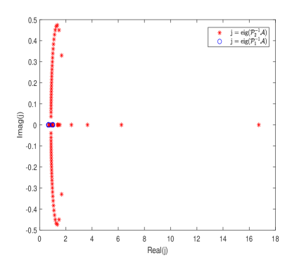
Theorem 3.1 implies that the generalized minimal residual (GMRES) method by Saad and Schultz [56] can compute the exact solution of the preconditioned system $\mathcal{P}^{-1}_{\alpha}\mathcal{A}$ (if it is diagonalizable) in at most $2N_{t}+1$ iterations [56, 23, 33]. Although it should be noted that such a convergence behavior of the preconditioned GMRES is not sharp when $N_{t}$ is not small, the result can give useful clues on the effectiveness of the preconditioner $\mathcal{P}_{\alpha}$ to approximate the all-at-once matrix $\mathcal{A}$. Moreover, in Section 4 we will show numerically that most of the eigenvalues of the preconditioned matrix $\mathcal{P}^{-1}_{\alpha}\mathcal{A}$ actually cluster at point 1 of the spectrum, supporting the theoretical findings of this section on the good potential of the proposed preconditioner $\mathcal{P}_{\alpha}$ to accelerate the iterative solution of $\mathcal{P}^{-1}_{\alpha}\mathcal{A}$.

References

- [1] S.Ş. Bayın, Definition of the Riesz derivative and its application to space fractional quantum mechanics, J. Math. Phys., 57(12) (2016), Article No. 123501, 12 pages. DOI: 10.1063/1.4968819.
- [2] R.L. Magin, Fractional Calculus in Bioengineering, Begell House Publishers, Danbury, CT (2006).
- [3] M.M. Meerschaert, C. Tadjeran, Finite difference approximations for two-sided space-fractional partial differential equations, Appl. Numer. Math., 56(1) (2006), pp. 80-90.
- [4] E. Scalas, R. Gorenflo, F. Mainardi Fractional calculus and continuous-time finance, Physica A, 284(1-4) (2000), pp. 376-384.
- [5] A.A. Kilbas, H.M. Srivastava, J.J. Trujillo, Theory and applications of fractional differential equations, Elsevier, Amsterdam, Netherlands (2006).
- [6] R. Metzler, J. Klafter, The random walk’s guide to anomalous diffusion: a fractional dynamics approach, Phys. Rep., 339(1) (2000), pp. 1-77.
- [7] M. Chen, Y. Wang, X. Cheng, W. Deng, Second-order LOD multigrid method for multidimensional Riesz fractional diffusion equation, BIT, 54(3) (2014), pp. 623-647.
- [8] C. Çelik, M. Duman, Crank-Nicolson method for the fractional diffusion equation with the Riesz fractional derivative, J. Comput. Phys., 231(4) (2012), pp. 1743-1750.
- [9] W.Y. Tian, H. Zhou, W. Deng, A class of second order difference approximations for solving space fractional diffusion equations, Math. Comp., 84(294) (2015), pp. 1703-1727.
- [10] H.-L. Liao, P. Lyu, S. Vong, Second-order BDF time approximation for Riesz space-fractional diffusion equations, Int. J. Comput. Math., 95(1) (2018), pp. 144-158.
- [11] D. Hu, X. Cao, A fourth-order compact ADI scheme for two-dimensional Riesz space fractional nonlinear reaction-diffusion equation, Int. J. Comput. Math., 97(9) (2020), pp. 1928-1948. DOI: 10.1080/00207160.2019.1671587.
- [12] X. Yue, S. Shu, X. Xu, W. Bu, K. Pan, Parallel-in-time multigrid for space-time finite element approximations of two-dimensional space-fractional diffusion equations, Comput. Math. Appl., 78(11) (2019), pp. 3471-3484.
- [13] Y. Xu, Y. Zhang, J. Zhao, Backward difference formulae and spectral Galerkin methods for the Riesz space fractional diffusion equation, Math. Comput. Simul., 166 (2019), pp. 494-507.
- [14] Y. Xu, Y. Zhang, J. Zhao, General linear and spectral Galerkin methods for the Riesz space fractional diffusion equation, Appl. Math. Comput., 364 (2020), Article No. 124664, 12 pages. DOI: 10.1016/j.amc.2019.124664.
- [15] J. Zhao, Y. Zhang, Y. Xu, Implicit Runge-Kutta and spectral Galerkin methods for Riesz space fractional/distributed-order diffusion equation, Comput. Appl. Math., 39(2) (2020), Article No. 47, 27 pages. DOI: 10.1007/s40314-020-1102-3.
- [16] H.-K. Pang, H.-W. Sun, Fast numerical contour integral method for fractional diffusion equations, J. Sci. Comput., 66(1) (2016), pp. 41-66.
- [17] M.J. Gander, M. Neumüller, Analysis of a new space-time parallel multigrid algorithm for parabolic problems, SIAM J. Sci. Comput., 38(4) (2016), pp. A2173-A2208.
- [18] R.D. Falgout, M. Lecouvez, C.S. Woodward, A parallel-in-time algorithm for variable step multistep methods, J. Comput. Sci., 37 (2019), Article No. 101029, 12 pages. DOI: 10.1016/j.jocs.2019.101029.
- [19] S.-L. Wu, T. Zhou, Acceleration of the MGRiT algorithm via the diagonalization technique, SIAM J. Sci. Comput., 41(5) (2019), pp. A3421-A3448.
- [20] M.E. Farquhar, T.J. Moroney, Q. Yang, I.W. Turner, GPU accelerated algorithms for computing matrix function vector products with applications to exponential integrators and fractional diffusion, SIAM J. Sci. Comput., 38(3) (2016), pp. C127-C149.
- [21] S.-L. Wu, T. Zhou, Fast parareal iterations for fractional diffusion equations, J. Comput. Phys., 329 (2017), pp. 210-226.
- [22] Y. Maday, E.M. Rønquist, Parallelization in time through tensor-product space-time solvers, C. R. Math., 346(1-2) (2008), pp. 113-118.
- [23] X.-M. Gu, T.-Z. Huang, X.-L. Zhao, H.-B. Li, L. Li, Strang-type preconditioners for solving fractional diffusion equations by boundary value methods, J. Comput. Appl. Math., 277 (2015), pp. 73-86.
- [24] M.J. Gander, 50 Years of Time Parallel Time Integration, in Multiple Shooting and Time Domain Decomposition Methods (T. Carraro, M. Geiger, S. Körkel, et al., eds.), Contributions in Mathematical and Computational Sciences, vol 9. Springer, Cham, Switzerland (2017), pp. 69-113. DOI: 10.1007/978-3-319-23321-5_3.
- [25] S.-L. Lei, Y.-C. Huang, Fast algorithms for high-order numerical methods for space-fractional diffusion equations, Int. J. Comput. Math., 94(5) (2017), pp. 1062-1078.
- [26] T. Breiten, V. Simoncini, M. Stoll, Low-rank solvers for fractional differential equations, Electron. Trans. Numer. Anal., 45 (2016), pp. 107-132.
- [27] A.T. Weaver, S. Gürol, J. Tshimanga, M. Chrust, A. Piacentini, “Time”-parallel diffusion-based correlation operators, Q. J. R. Meteorol. Soc., 144(716) (2018), pp. 2067-2088.
- [28] D. Bertaccini, F. Durastante, Block structured preconditioners in tensor form for the all-at-once solution of a finite volume fractional diffusion equation, Appl. Math. Lett., 95 (2019), pp. 92-97.
- [29] I. Podlubny, A. Chechkin, T. Skovranek, Y.Q. Chen, B.M.V. Jara, Matrix approach to discrete fractional calculus II: Partial fractional differential equations, J. Comput. Phys., 228(8) (2009), pp. 3137-3153.
- [30] M. Ran, C. Zhang, A high-order accuracy method for solving the fractional diffusion equations, J. Comp. Math., 38(2) (2020), pp. 239-253.
- [31] L. Banjai, D. Peterseim, Parallel multistep methods for linear evolution problems, IMA J. Numer. Anal., 32(3) (2012), pp. 1217-1240.
- [32] Y.-L. Zhao, P.-Y. Zhu, X.-M. Gu, X.-L. Zhao, H.-Y. Jian, A preconditioning technique for all-at-once system from the nonlinear tempered fractional diffusion equation, J. Sci. Comput., 83(1) (2020), Article No. 10, 27 pages. DOI: 10.1007/s10915-020-01193-1.
- [33] E. McDonald, J. Pestana, A. Wathen, Preconditioning and iterative solution of all-at-once systems for evolutionary partial differential equations, SIAM J. Sci. Comput., 40(2) (2018), pp. A1012-A1033.
- [34] A. Goddard, A. Wathen, A note on parallel preconditioning for all-at-once evolutionary PDEs, Electron. Trans. Numer. Anal., 51 (2019), pp. 135-150.
- [35] X.-L. Lin, M. Ng, An all-at-once preconditioner for evolutionary partial differential equations, arXiv preprint, arXiv:2002.01108, submitted to SIAM J. Sci. Comput., 4 Feb. 2020, 17 pages.
- [36] S.-L. Wu, H. Zhang, T. Zhou, Solving time-periodic fractional diffusion equations via diagonalization technique and multigrid, Numer. Linear Algebra Appl., 25(5) (2018), Article No. e2178, 24 pages. DOI: 10.1002/nla.2178.
- [37] O. Bokanowski, K. Debrabant, Backward differentiation formula finite difference schemes for diffusion equations with an obstacle term, IMA J. Numer. Anal., to appear, 6 Jul. 2020, 29 pages. DOI: 10.1093/imanum/draa014.
- [38] M. Donatelli, M. Mazza, S. Serra-Capizzano, Spectral analysis and structure preserving preconditioners for fractional diffusion equations, J. Comput. Phys., 307 (2016), pp. 262-279.
- [39] K. Burrage, Parallel and Sequential Methods for Ordinary Differential Equations, Oxford University Press, New York, NY (1995).
- [40] U.M. Ascher, L.R. Petzold, Computer Methods for Ordinary Differential Equations and Differential-Algebraic Equations, SIAM, Philadelphia, PA (1998).
- [41] C. Lubich, D. Mansour, C. Venkataraman, Backward difference time discretization of parabolic differential equations on evolving surfaces, IMA J. Numer. Anal., 33(4) (2013), pp. 1365-1385.
- [42] E. Emmrich, Error of the two-step BDF for the incompressible Navier-Stokes problem, ESAIM-Math. Model. Numer. Anal., 38(5) (2004), 757-764.
- [43] V. Kučera, M. Vlasák, A priori diffusion-uniform error estimates for nonlinear singularly perturbed problems: BDF2, midpoint and time DG, ESAIM-Math. Model. Numer. Anal., 51(2) (2017), pp. 537-563.
- [44] H. Nishikawa, On large start-up error of BDF2, J. Comput. Phys., 392 (2019), pp. 456-461.
- [45] Q. Zhang, Y. Ren, X. Lin, Y. Xu, Uniform convergence of compact and BDF methods for the space fractional semilinear delay reaction-diffusion equations. Appl. Math. Comput., 358 (2019), pp. 91-110.
- [46] C. Li, M.-M. Li, X. Sun, Finite difference/Galerkin finite element methods for a fractional heat conduction-transfer equation, Math. Meth. Appl. Sci., to appear, 30 Oct. 2019, 20 pages. DOI: 10.1002/mma.5984.
- [47] D. Bini, F. Di Benedetto, A new preconditioner for the parallel solution of positive definite Toeplitz systems, Proceedings of the Second Annual ACM Symposium on Parallel Algorithms and Architectures (SPAA ’90), ACM, New York, NY (1990), pp. 220-223. DOI: 10.1145/97444.97688.
- [48] F. Di Benedetto, Preconditioning of block Toeplitz matrices by sine transforms, SIAM J. Sci. Comput., 18(2) (1997), pp. 499-515.
- [49] S. Serra, Superlinear PCG methods for symmetric Toeplitz systems, Math. Comp., 68(226) (1999), pp. 793-803.
- [50] Z. Hao, Z. Zhang, R. Du, Fractional centered difference scheme for high-dimensional integral fractional Laplacian, J. Comput. Phys., 424 (2021), Article No. 109851, 17 pages. DOI: 10.1016/j.jcp.2020.109851.
- [51] Q. Yang, F. Liu, I. Turner, Numerical methods for fractional partial differential equations with Riesz space fractional derivatives, Appl. Math. Model., 34(1) (2010), pp. 200-218.
- [52] Z.-P. Hao, Z.-Z. Sun, W.-R. Cao, A fourth-order approximation of fractional derivatives with its applications, J. Comput. Phys., 281 (2015), pp. 787-805.
- [53] W.W. Hager, Updating the inverse of a matrix, SIAM Rev. 31(2) (1989), pp. 221-239.
- [54] X.-M. Gu, S.-L. Wu, A parallel-in-time iterative algorithm for Volterra partial integro-differential problems with weakly singular kernel, J. Comput. Phys., 417 (2020), Article No. 109576, 17 pages. DOI: 10.1016/j.jcp.2020.109576.
- [55] P. Jiránek, M. Rozložník, Adaptive version of Simpler GMRES, Numer. Algorithms, 53(1) (2010), pp. 93-112.
- [56] Y. Saad, Iterative Methods for Sparse Linear Systems, 2nd ed., SIAM, Philadelphia, PA (2003).
- [57] M.J. Gander, L. Halpern, Time parallelization for nonlinear problems based on diagonalization, in Domain Decomposition Methods in Science and Engineering XXIII (C.-O. Lee, X.-C. Cai, D.E. Keyes, et al., eds.), Lecture Notes in Computational Science and Engineering, vol. 116, Springer, Cham, Switzerland (2017), pp. 163-170. DOI: 10.1007/978-3-319-52389-7_15.