No.299 Bayi Road, Wuhan 430072, Chinabbinstitutetext: Hubei Key Laboratory of Nuclear Solid Physics, School of Physics and Technology, Wuhan University,
No.299 Bayi Road, Wuhan 430072, China
A note on multi-trace EYM amplitudes in four dimensions
Abstract
In four dimensions, a tree-level double-trace Einstein-Yang-Mills (EYM) amplitude with two negative-helicity gluons (the -configuration) satisfies a symmetric spanning forest formula, which was derived from the graphic expansion rule. On another hand, in the framework of Cachazo-He-Yuan (CHY) formula, the maximally-helicity-violating (MHV) amplitudes are supported by the MHV solution of scattering equations. The relationship between the symmetric formula for double-trace amplitudes, and the MHV sector of Cachazo-He-Yuan (CHY) formula in four dimensions is still not clear. In this note, we promote a series of transformations of the spanning forests in four dimensions and then show a systematic way for decomposing the MHV sector of the CHY formula of double-trace EYM amplitudes. Along this line, the symmetric formula of double-trace MHV amplitudes is directly obtained by the MHV sector of CHY formula. We then prove that EYM amplitude with an arbitrary total number of negative-helicity particles (gravitons and gluons) has to vanish when the number of negative- (or positive-) helicity gluons is less than the number of traces.
Keywords:
Scattering Amplitudes, Gauge Symmetry1 Introduction
The expansion of Einstein-Yang-Mills (EYM)222In this paper, B-field and dilaton are also involved in the theory. amplitudes states that tree-level EYM amplitudes can be expanded in terms of color-ordered Yang-Mills (YM) amplitudes. This expansion was first observed for single-trace amplitudes with one graviton Stieberger:2016lng , then extended to amplitudes with a few gravitons and gluon traces Nandan:2016pya ; Schlotterer:2016cxa . General patterns of the expansions based on a recursive expression were established for not only single-trace amplitudes Fu:2017uzt ; Chiodaroli:2017ngp ; Teng:2017tbo but also multi-trace ones Du:2017gnh . These expansion formulas provided a new angle for understanding several related problems, including: constructing local Bern-Carrasco-Johansson (BCJ) Bern:2008qj numerators Fu:2017uzt ; Du:2017kpo ; Du:2018khm , inducing new amplitude relations by gauge symmetries Fu:2017uzt ; Du:2017kpo ; Du:2018khm ; Hou:2018bwm ; Du:2019vzf , providing an off-shell approach to BCJ duality (and amplitude relations) Wu:2021exa ; Du:2022vsw and evaluating EYM amplitudes in four dimensions Tian:2021dzf . Several discussions at loop amplitudes can also be found (see Porkert:2022efy ; Zhou:2022djx ; Faller:2018vdz for example).
Among the above progresses on the expansion of EYM amplitudes, a symmetric formula of maximally-helicity-violating (MHV) double-trace EYM amplitudes in four dimensions was proposed Tian:2021dzf . In this formula, the two gluon traces are given by two Parke-Taylor Parke:1986gb factors, while gravitons are included by spanning forests that are rooted at gluons. A key feature of this formula is that either the two traces or the gravitons are arranged in an equal footing. Such symmetric pattern was earlier discovered for the tree-level gravity (GR) amplitudes Nguyen:2009jk ; Hodges:2012ym ; Feng:2012sy , the tree-level single-trace EYM amplitudes Du:2016wkt as well as the double-trace pure gluon amplitudes in EYM theory Cachazo:2014nsa , with the MHV configurations.
Apart from the line of EYM expansion, the famous Cachazo-He-Yuan (CHY) Cachazo:2013gna ; Cachazo:2013hca ; Cachazo:2013iea ; Cachazo:2014nsa ; Cachazo:2014xea formula provides another powerful approach to the calculations in four dimensions. By CHY formula, one can substitute the MHV solution (i.e. the solution supporting the MHV amplitudes) of the scattering equations (SE) into the CHY integrand, which involves a Pfaffian and a reduced Pfaffian, straightforwardly and then expand the integrand in a proper way to obtain an expression of MHV amplitudes. This approach verifies the fact that the MHV solution supports the MHV amplitudes. Along this line, the tree-level MHV amplitudes of YM, GR and the single-trace MHV EYM amplitudes have been already evaluated Du:2016blz ; Du:2016wkt . Nevertheless, there are still gaps between the symmetric formula proposed in Tian:2021dzf and the direct evaluation of the CHY formula for double-trace MHV amplitudes. First, the two traces in the CHY formula do not stand in an equal status, in the sense that the Pfaffian part in CHY formula only involves gluons from one trace. Thus the relationship between the MHV sector of CHY formula and the symmetric formula in Tian:2021dzf is not transparent. Second, in Weinzierl:2014vwa ; Du:2016fwe , it was explicitly shown that the reduced Pfaffian with two negative-helicity particles is supported by the MHV solution to SE333Studies of solutions to SE from distinct aspects can be found in the work Roberts:1972abc ; Fairlie:1972abc ; Fairlie:2008dg ; Cachazo:2013hca ; Cachazo:2013gna ; Monteiro:2013rya ; Geyer:2014fka ; Mason:2013sva ; Weinzierl:2014vwa ; Dolan:2015iln ; Cardona:2015ouc ; Cachazo:2016sdc ; He:2016vfi ; Du:2016fwe . by substituting the MHV solution into the reduced Pfaffian, but there are vanishing configurations Cachazo:2014xea ; Tian:2021dzf of multi-trace amplitudes with two negative-helicity particles. More generally, the vanishing configurations for amplitudes with an arbitrary number of negative-helicity particles for GR, YM, single-trace EYM amplitudes and pure gluon multi-trace EYM were already understood in a way via considering the rank of a discriminant matrix (see Cachazo:2014xea for the pure-gluon multi-trace case and Du:2016fwe for the single-trace EYM cases with gravitons). However, these arguments have not been extended to multi-trace cases with an arbitrary number of gravitons yet. In this note, we fill these two gaps. By breaking the symmetry between the two traces and proposing a new formula of double-trace MHV amplitudes, we find the connection between the MHV sector of CHY formula and the symmetric formula of double-trace amplitudes Tian:2021dzf . We further prove that amplitudes with an arbitrary number of negative- (positive-) helicity particles have to vanish when the number of negative- (and/or positive-) helicity gluons is less than the number of gluon traces. This is a complement of the discussion on the vanishing configurations Cachazo:2014xea ; Du:2016fwe .
The structure of this note is arranged as follows. In section 2, we introduce several helpful transformations of the spanning forests and then prove a new formula of double-trace MHV amplitude with two negative-helicity gluons, by breaking the symmetry between the two traces. In section 3, we derive the formula proposed in section 2 along the other line, i.e. the CHY approach, by substituting the MHV solution to SE into Pfaffian. The vanishing configurations for an arbitrary number of negative-helicity particles are studied in section 4. Conclusions of this note are provided in section 5. A one-graviton example for the proof in section 2.2 and the vanishing condition of a determinant introduced in section 4 are provided in the appendix.
2 A new formula of double-trace MHV amplitudes with -configuration
In EYM theory, a tree-level double-trace MHV amplitude (, are the two negative-helicity gluons) with two gluon traces , and the graviton set satisfies the following symmetric spanning forest formula Tian:2021dzf
| (2.1) | |||||
which is written by spinor products Xu:1986xb . On the RHS, the prefactor involves two Parke-Taylor Parke:1986gb factors which encode permutations of gluons in the traces, while the expression in the square brackets is interpreted by spanning forests where gluons and gravitons are considered as nodes. The spanning forests are generated by the following steps:
-
•
Step-1 Split the graviton set into two subsets and .
-
•
Step-2 Choose a pair of gluons , . Construct a path towards passing through some elements of , and a path towards passing through the remaining elements of . Connecting the starting nodes and of the two paths, one obtains a bridge between the two traces.
-
•
Step-3 For a given bridge constructed by the previous step, generate a spanning forest which connects the gravitons in to roots (i.e. gluons and the gravitons on the bridge) via tree structures.
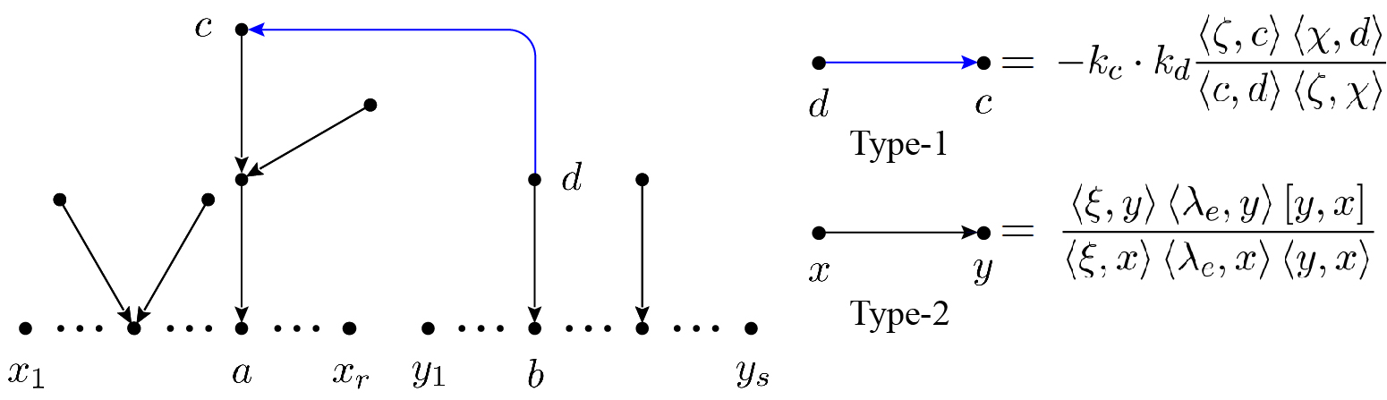
A spanning forest, as shown in Fig. 1, that is generated by the above steps contributes the product of the factors corresponding to each edge. The edge between the nodes and in step-2 (the blue edge in Fig. 1) is called type-1 edge and is accompanied by a factor
| (2.2) |
while other edges pointing from to correspond to
| (2.6) |
are mentioned as type-2 edges. Here, the set of edges on the bridge pointing to the trace and the trace are denoted by and , respectively, while the set of other edges are denoted by . The , , and are arbitrarily chosen (but to avoid the divergence in (2.2)) reference spinors which reflect symmetries of the amplitude Tian:2021dzf . For convenience, we set in this paper. Under this choice, the gauges for edges in and are identical but they are distinct from those for . A typical forest is given by Fig. 1.
In this section, we introduce the following new formula for double-trace MHV amplitudes
| (2.7) | |||||
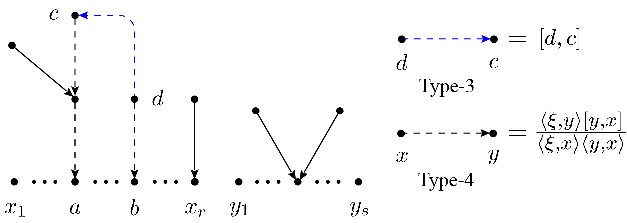
which is equivalent to eq. (2.1). Being different from eq. (2.1), the above equation is based on spanning forests consisting of two mutually disjoint components, which correspond to the two gluon traces, as shown by Fig. 2. In Fig. 2, the two ending nodes and of the bridge now become gluons belonging to the same trace and the node is always nearer to the gluon than the node . The bridge in Fig. 2 is expressed by type-3 and -4 edges , instead, which correspond to the factors , . Other nodes are connected to gluon traces or bridge through type-2 edges.
In the following, helpful transformations satisfied by the spanning forests are introduced, by which we prove that the formula (2.1) where the bridge is constructed between distinct traces can be transformed into the formula (2.7) where both ends of the bridge are moved to a single trace.
2.1 Transformations of spanning forests
To show the two formulas (2.1) and (2.7) are equivalent to each other, we introduce the following three transformations of spanning forests.
Transformation-1:
When the in (2.2) is expressed by spinor products, the expression corresponding to the structure on the LHS of Fig. 3 is given by
| (2.8) |
Note that the minus of the factor for the type-3 edge is absorbed due to the antisymmetry of the spinor product . After dividing out the common factors in the numerator and denominator, the factors involving the reference spinors and are collected as
| (2.9) |
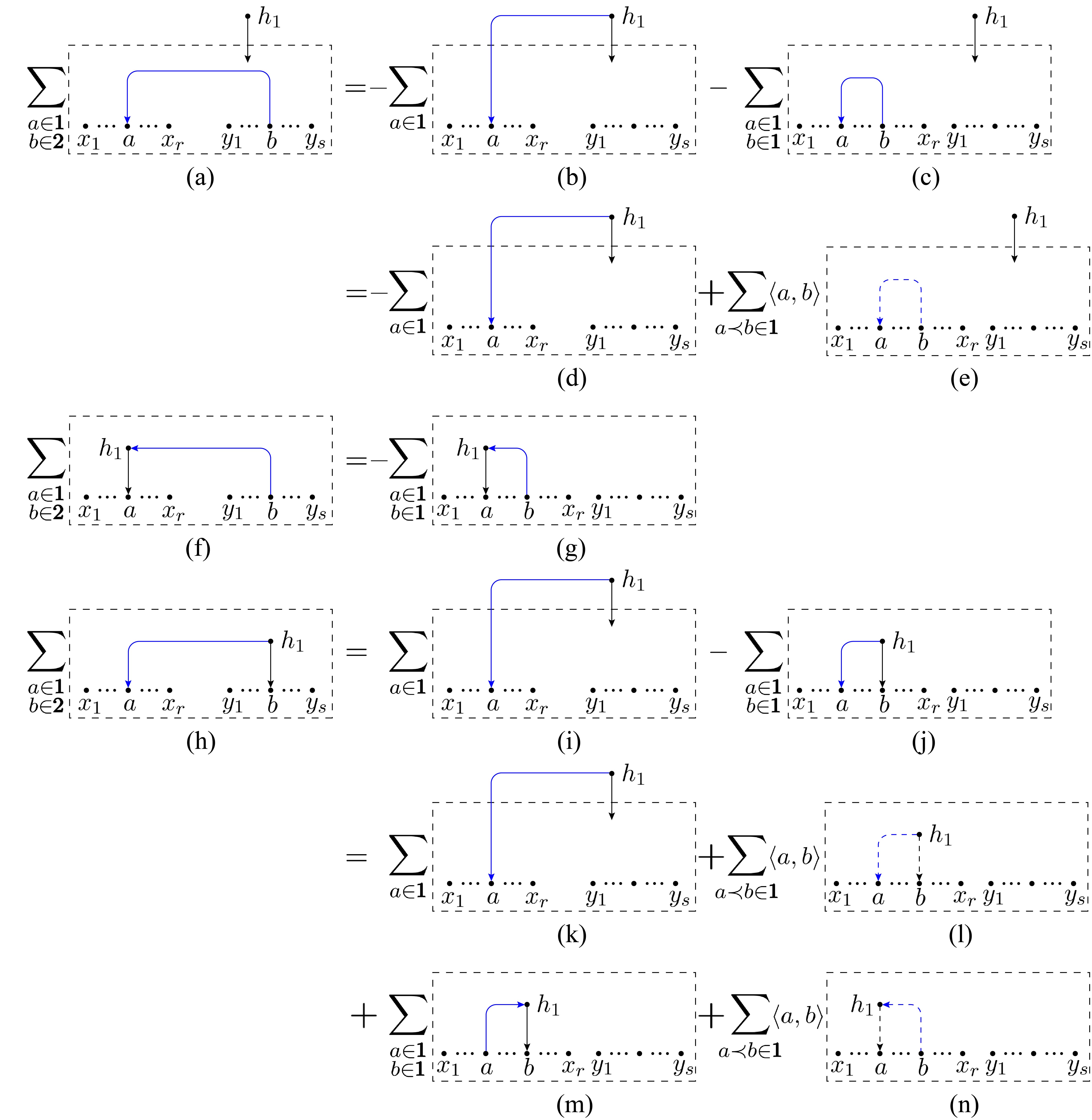
where the Schouten identity has been applied. When the RHS of eq. (2.9) are inserted, the expression (2.8) splits into two terms corresponding to the graphs on the RHS of Fig. 3, where the first contains the type-3 and -4 edges introduced in eq. (2.7) and the second still contains the type-1 and -2 edges in eq. (2.1) but the choices of gauge on both sides of the type-1 edge are exchanged.
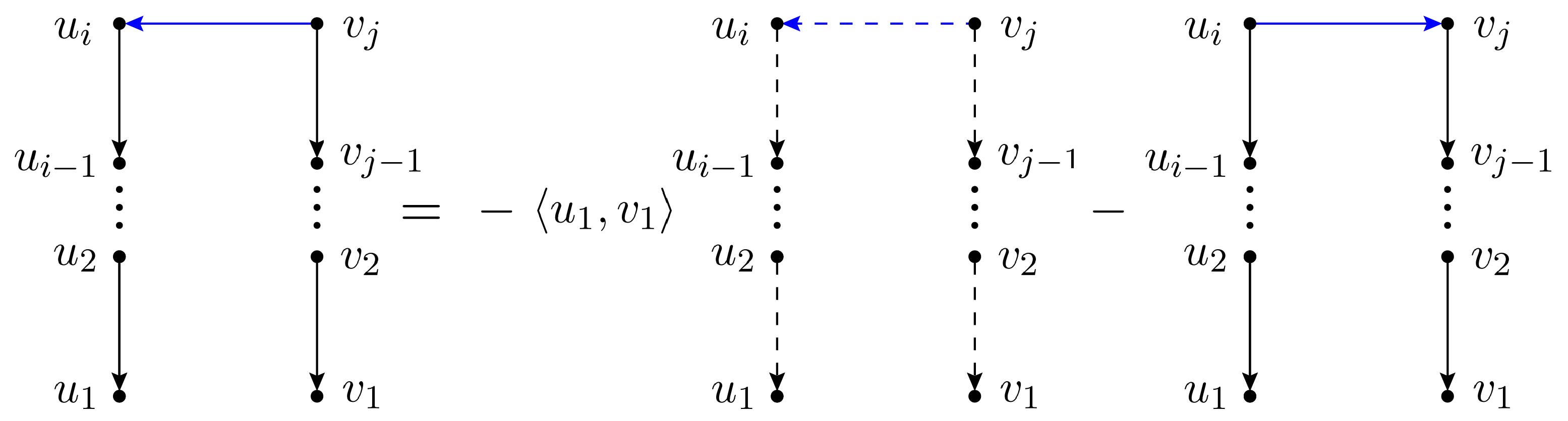
Transformation-2:
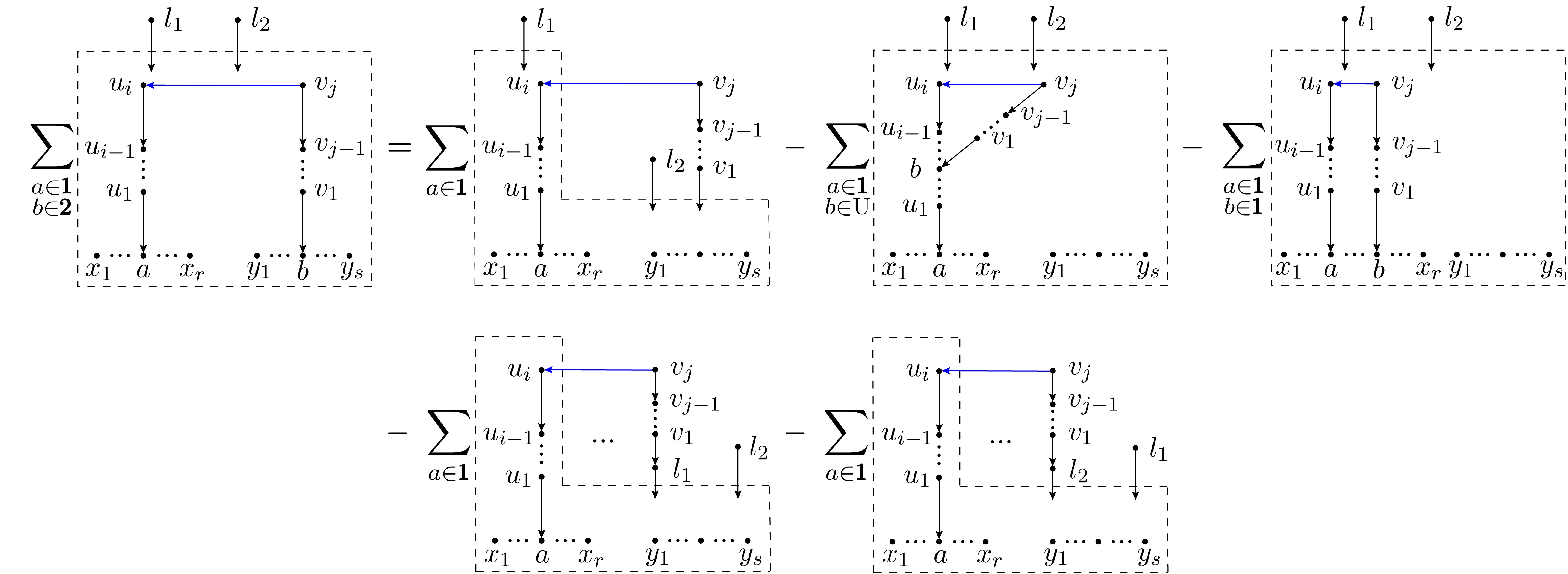
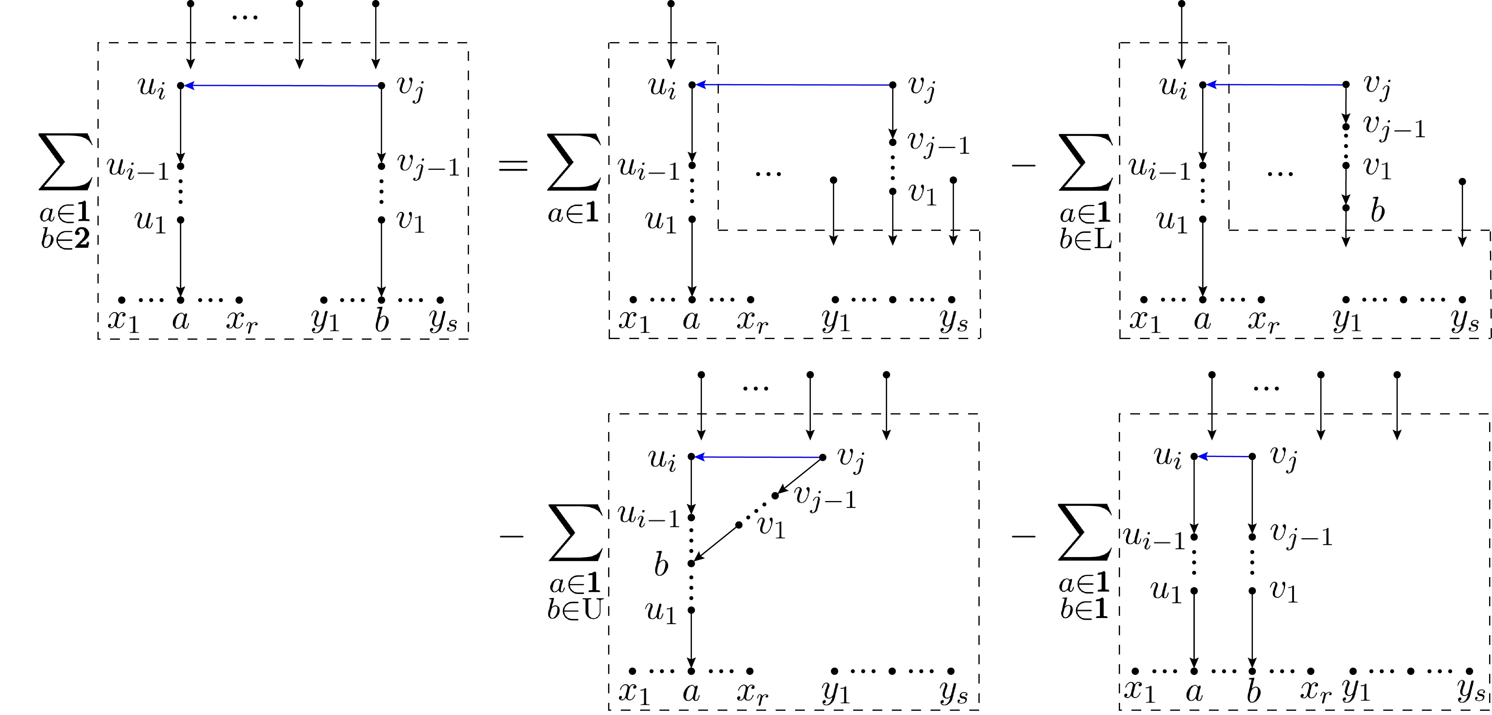
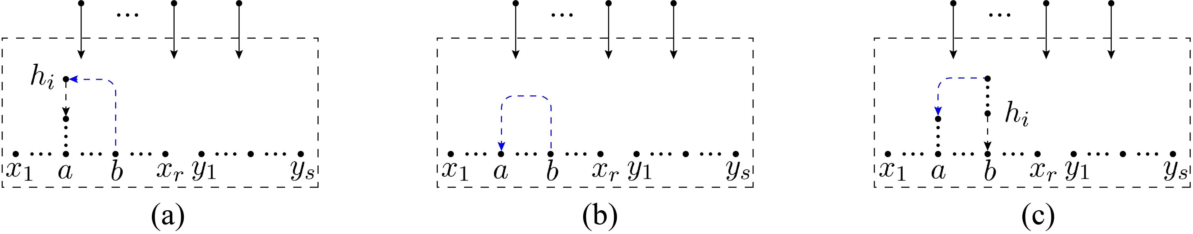
For given , on the LHS of Fig. 4, all nodes in the boxed region are considered as roots. Other nodes are connected to the roots via tree structures. The summation over all possible such spanning forests are implied by the box. In the first graph on the RHS, we sum over all possible spanning forests with keeping the chain structure and then connect the node to via a type-1 edge. The contributions where (the root of the chain ) is (i). a node outside the boxed regions, (ii). a node belonging to as well as (iii). a node in the trace are subtracted as the last three graphs on the RHS of Fig. 4. Then only the cases where is a node in trace survive, thus the equality of Fig. 4 holds. An explicit example for this transformation is given by Fig. 5: According to the definition, the first graph on the RHS of Fig. 4 where two gravitons and belong to the set (the set of gravitons that are not in set ) gives the equation of Fig. 5, which can be verified by moving the last four graphs on the RHS to the LHS.
Transformation-3:
If the set is empty, the first term on the RHS of transformation-2 contains a factor
| (2.10) |
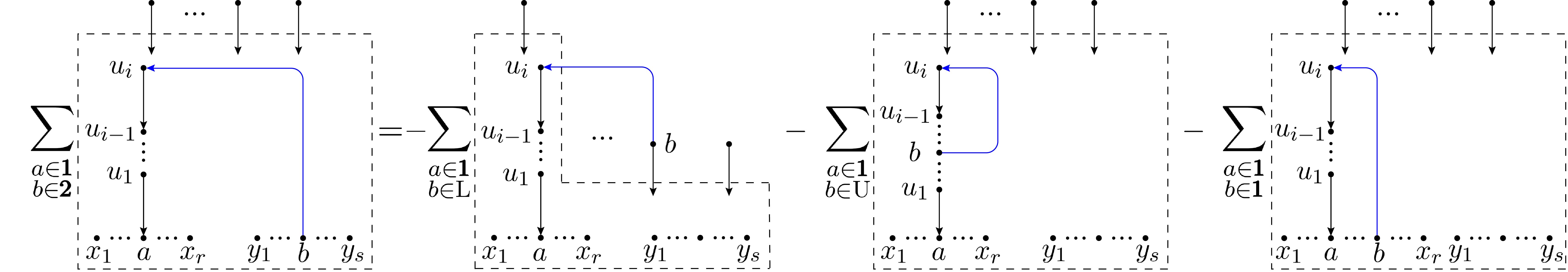
where momentum conservation has been applied. Transformation-2 then turns into the relation shown by Fig. 6.
2.2 The general proof
To prove the formula (2.7), we note that the RHS of (2.1) has the general pattern of the LHS of Fig. 4 or Fig. 6. One can therefore transform these factors according to transformation-2 and -3, whose terms on the RHS can be classified into the following three categories.
-
•
Category-1 The first two graphs on the RHS of Fig. 4 and the first graph on the RHS of Fig. 6 have a common structure: all possible spanning forests while a chain structure (, in the first two terms of Fig. 4 and the single node in Fig. 6) is preserved are summed over and the starting node of this chain is connected to via a type-1 edge. All these graphs belong to category-1.
- •
-
•
Category-3 In the last graph on the RHS of Fig. 4 and the last graph on the RHS of Fig. 6, all graphs where the chain pointing towards a gluon in trace are summed over. The starting node is also connected to , via a type-1 edge. Thus there is a bridge between two gluons belonging to the trace in such a graph.
Now let us track back to the origins of these graphs in distinct categories and see the cancellations among graphs:
-
•
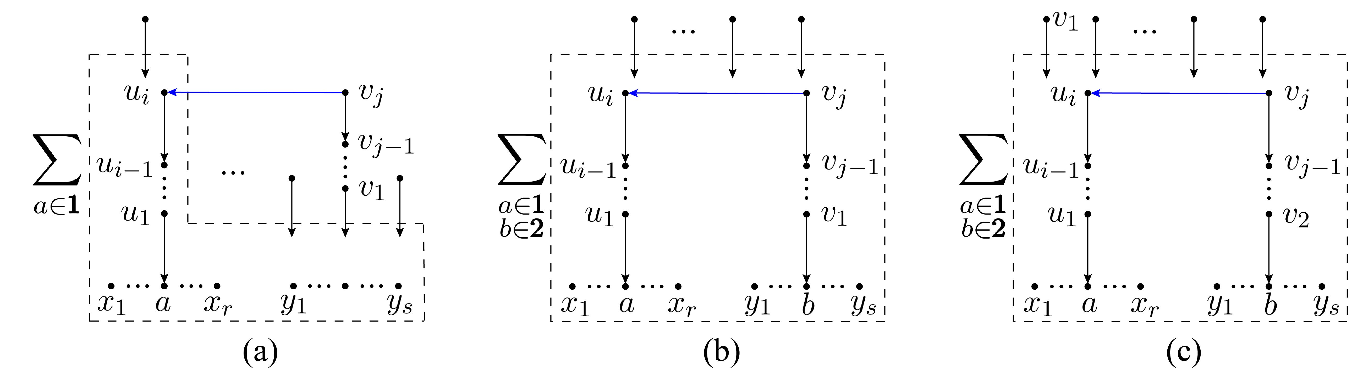
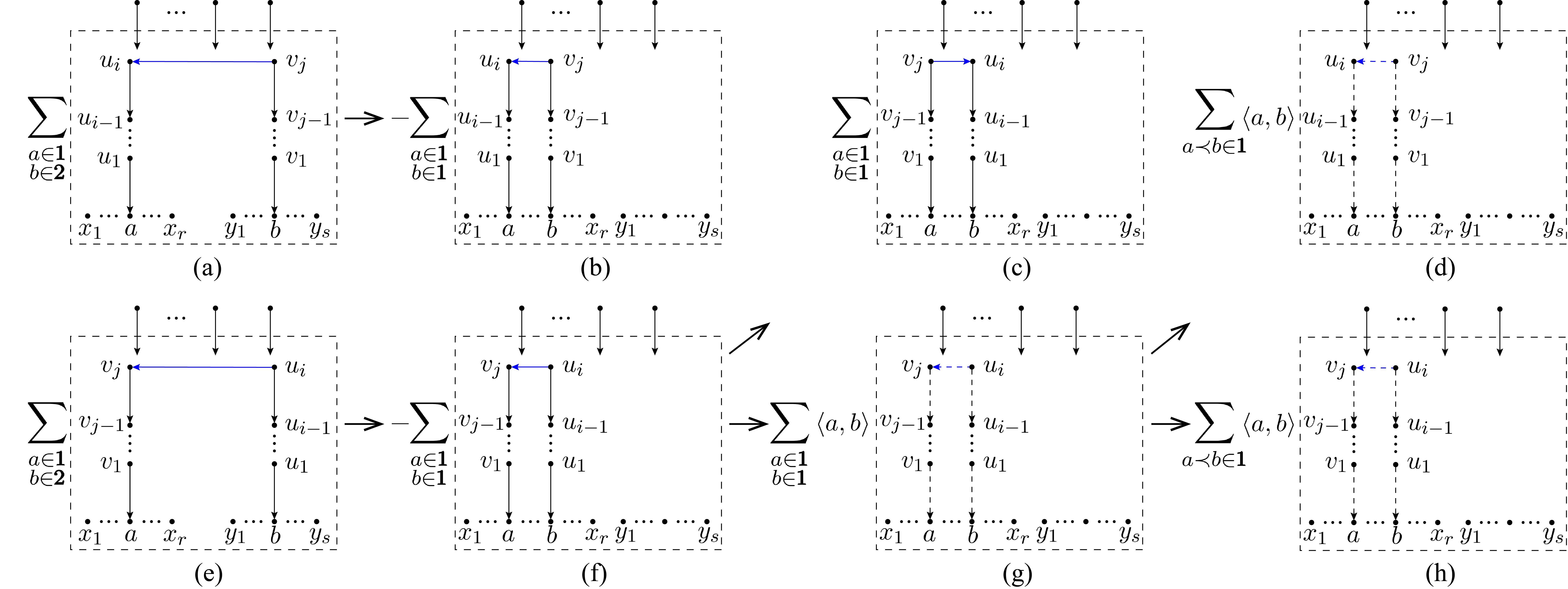
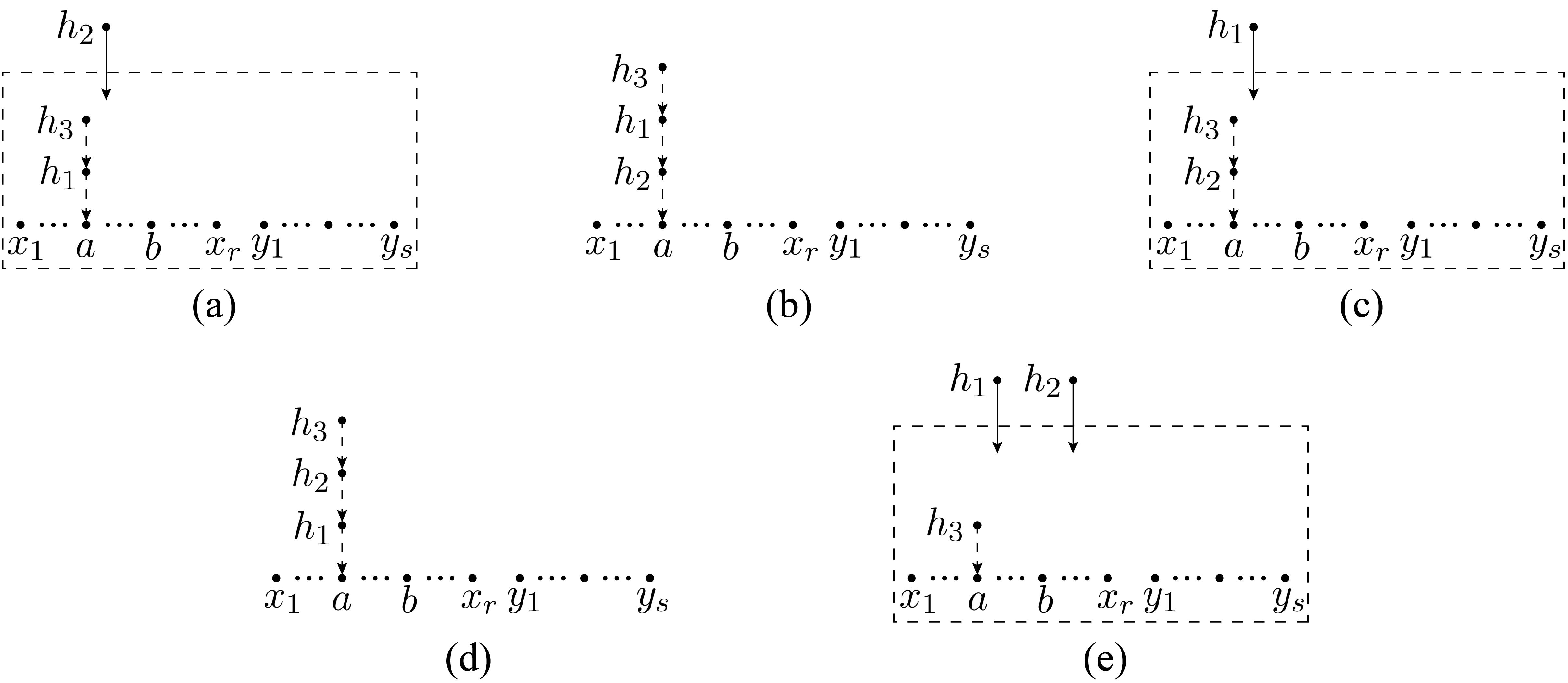
The typical graph of category-1 shown by Fig. 7 (a) where the nodes on the bridge between and are in turn, can only be obtained from the expansions of Fig. 7 (b) and (c). Since Fig. 7 (a) is the first term in the expansion of Fig. 7 (b) but the second term in the expansion of Fig. 7 (c) when transformation-2 is applied, one such figure must appear twice with opposite signs and then cancel in pairs.
-
•
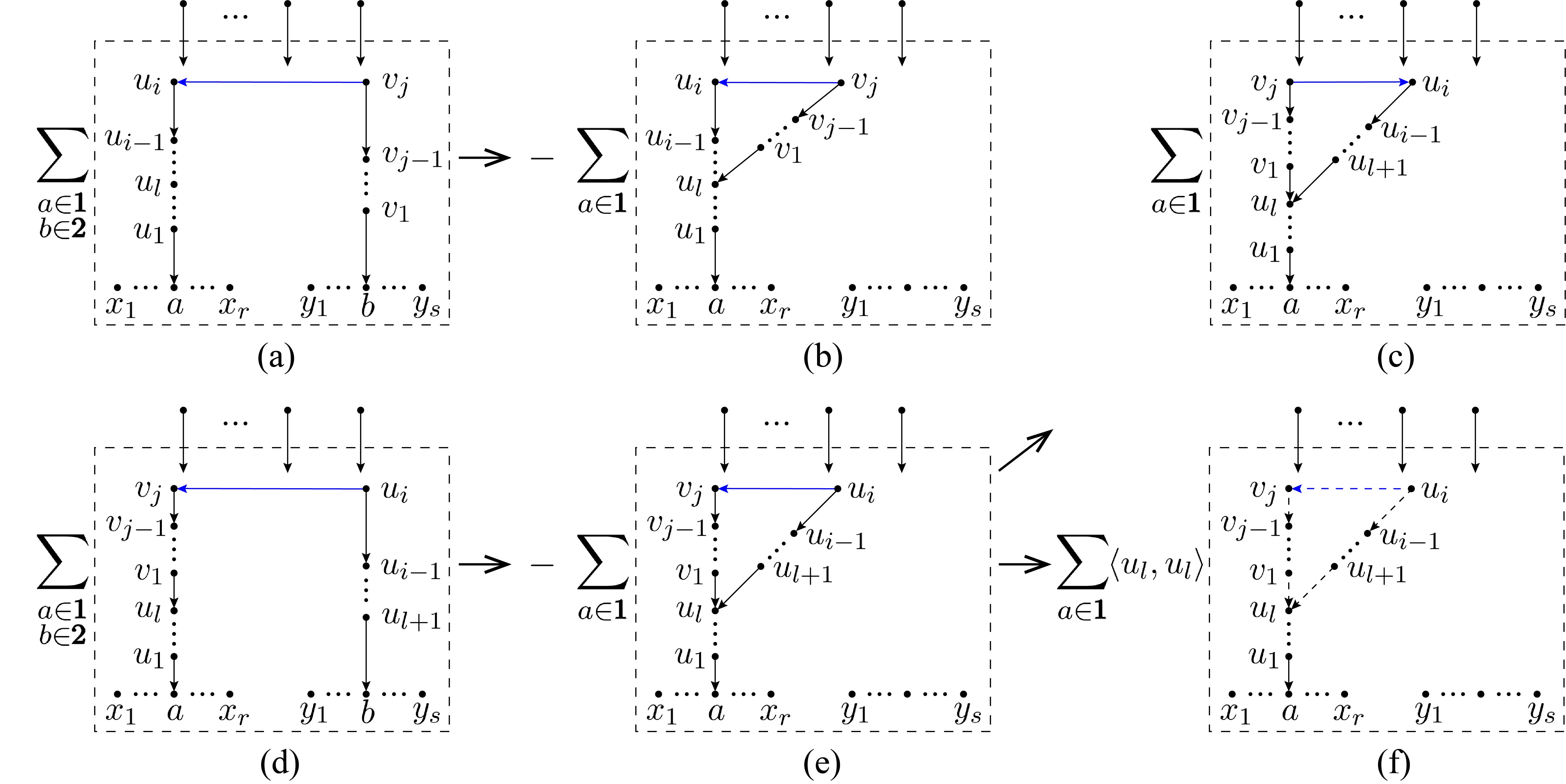
Graphs of category-2 appear in pairs as shown by Fig. 8 (b) and (e), which respectively come from the decomposition of spanning forests (a) and (d). These two graphs are related to one another by exchanging the roles between the chain structures and . The graph (e) further splits into the two graphs (c) and (f), when transformation-1 is applied. The graph (c) cancels with (b), while the graph (f) has to vanish due to the antisymmetry of spinor products. Thus graphs of category-2 have to cancel out.
-
•
Graphs of category-3 also come in pairs as shown by Fig. 9 (b) and (f), which are obtained from the spanning forests (a) and (e). When applying transformation-1 to the graph (f), one gets the two graphs (c) and (g). The graph (c) cancels with (b), while the graph (g) is further expanded into graphs (d) and (h). This is because the summation over can split as
(2.11) When , are renamed by , , respectively, the second summation on the RHS turns into a summation over but the structure between and is reflected, as shown by the graph (d) in Fig. 9 (the direction of the arrow line from to is adjusted by absorbing a minus into the coefficient ).
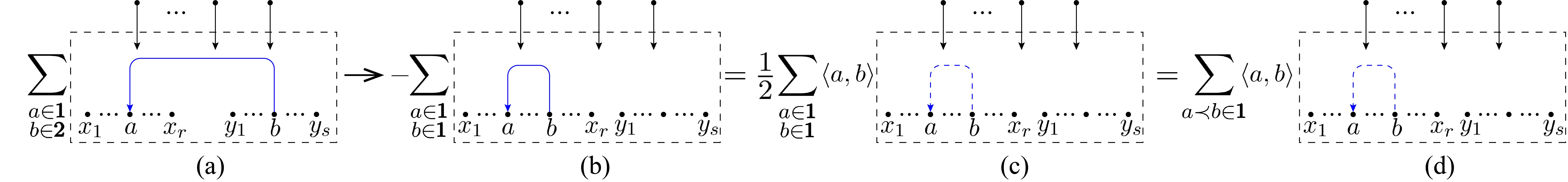
There is a boundary case of category-3 when both sets and are empty, as shown by the graph (b) in Fig. 10, which is obtained after applying transformation-3 to spanning forest (a). When we apply transformation-1 to this graph (b), the LHS of Fig. 3 is same with the second term on the RHS (upto a minus), thus the LHS is half of the first term on the RHS, as shown by the first equality of Fig. 10. The summation over all is further written as twice of the summation over ().
3 CHY approach to double-trace MHV amplitudes with two negative-helicity gluons
In this section, we evaluate the double-trace MHV amplitude in four dimensions by CHY formula directly. We straightforwardly substitute the MHV solution into the (integrated) CHY formula for double-trace amplitudes, then show that this sector reduces into the formula (2.7).
3.1 A review of the CHY formula for multi-trace EYM amplitudes
In the Cachazo-He-Yuan (CHY) framework, an -point scattering amplitude can be given by the following (integrated) formula
| (3.1) |
In the above expression:
-
•
One have summed over solutions () of the following scattering equations for scattering variables
(3.2) where and . In four dimensions, the scattering equations have a special solution (which is called MHV solution)
(3.3) where the spinors , and represent the Mbius freedom of scattering equations.
-
•
The reduced determinant is defined by
(3.4) where is the signature of the permutation that moves the standard ordering to and keeps ascending. The matrix is given by
(3.7) and is the submatrix obtained by removing the -th row and the -th column from .
-
•
The CHY integrand relies on theories. In EYM theory, the CHY integrand for color-odered -trace amplitudes have the following form
(3.8) where is the Parke-Taylor factor for the gluon trace and the reduced Pfaffian is defined as
(3.9) The is an antisymmetric matrix with the following structure
where the three blocks , and are matrices defined as follows
(3.16) The denotes half polarization of the graviton . In the integrand (3.8),
(3.17) where represents .
It is worth pointing out that Pfaffians can be defined recursively
| (3.18) |
A simple but helpful property is the following: if a antisymmetric matrix has the form
| (3.19) |
where both and are blocks, is an all-zero block. The Pfaffian of (3.19) can be reduced as
| (3.20) |
3.2 Evaluating the double-trace -amplitudes by CHY formula
Now let us evaluate the double-trace amplitude with -configuration by CHY formula straightforwardly. When the EYM integrand (3.8) for double-trace amplitude is substituted into the integrated expression (3.1), the amplitude becomes444The sign in (3.17) is absorbed if the , in the Pfaffian are arranged in canonical order.
| (3.21) |
For the sector supported by the MHV solution (3.3), we have
| (3.22) | |||||
where we omit the superscript of for convenience. In the above expression, we have used the property introduced in Du:2016wkt
| (3.23) |
where the , are the two negative-helicity particles, and
| (3.24) |
The submatrix of consists of three blocks , and . The indices of square matrices and correspondingly take values as (i). elements of in order, and (ii). elements in . The block is the submatrix of with row and column indices taking values in and respectively.
In the case that the negative-helicity particles , are gluons, the Lorentz contraction of momenta and polarizations in are expressed by
| (3.25) |
where we choose the reference spinor for all positive-helicity particles as , while that for the negative-helicity particles as . When and are extracted out from rows and columns in , respectively, the amplitude turns into
| (3.26) |
where
| (3.33) |
In the coming subsection, we prove that the summation in eq. (3.26) can be expanded into the expression inside the square brackets of eq. (2.7). Then the result from the MHV sector (i.e. the sector supported by the MHV solution) of CHY formula precisely reduces into the expansion formula (2.7) and is therefore equivalent to the spanning forest form (2.1).
3.3 The expansion of
In this subsection, we expand the and show that this expansion results in the expression in the square brackets of eq. (2.7). We first provide the examples with one and two gravitons, then the general proof.
One-graviton case
The simplest example is the Pfaffian involving one graviton , which is explicitly written as
| (3.34) |
According to the recursive expression (3.18), the Pfaffian can be given by
| (3.35) |
where . The above three terms correspond to the three graphs in Fig. 11 which describe the expansion formula (2.7) with one graviton.
Two-graviton case
The with two gravitons are explicitly given by
| Pf | (3.36) | ||||
where the recursive expansion of Pfaffian (3.18) is applied again. The - are reduced as follows:
- •
-
•
The factor in the third term on the RHS of (3.36) has the following form
(3.38) Since the Hodges determinant Hodges:2012ym is defined as
(3.39) where the reference spinors and are arbitrarily chosen, the determinant is equivalent to the Hodges determinant with two gravitons and . The spanning forest Nguyen:2009jk ; Feng:2012sy corresponding to the Hodges determinant, together with the factor , is shown by Fig. 12 (b).

Figure 13: All two-graviton graphs with () directly connected to via a type-4 edge -
•
and The last two factors and on the RHS of (3.36) are given by
(3.40) Note that (and ) can be obtained by performing the replacements , ( ) simultaneously on the Pfaffian with one graviton, which was already expanded as Fig. 11. When multiplied by the corresponding factor in eq. (3.36) (i.e. the edge between () and ), (and ) becomes terms characterized by Fig. 13.
To summarize, all terms in the expansion of correspond to the graphs Fig. 12 and Fig. 13, which are all contributions of (2.7) for amplitude with two gravitons.
General expansion
The -graviton Pfaffian for double-trace amplitudes is explicitly displayed as
| Pf | (3.51) |
Inspired by the two-graviton example, we expand this Pfaffian by entries on the -th row into three parts:
Part-1: the part involving all terms with . Such a term is given by the Pfaffian of the matrix when the two rows and two columns with respect to and are deleted. Since the new matrix has the form (3.19), according to eq. (3.20), the expansion coefficient of reduces into the determinant of a matrix, as follows
| (3.53) |
To show the expansion of this determinant, let us have a look at the , example. This determinant can be expanded by the third row
| (3.54) | |||||
where the two second-order determinants in the first two terms have the same pattern (3.53), while the last term involves a Hodges determinant. Substituting the corresponding diagram Fig. 12 (a) for the second-order determinant into the first two terms respectively, one reduces the first two terms into (a), (b) and (c), (d) in Fig. 14. The Hodges determinant can be expanded into the sum of all possible diagrams where all gluons play as roots and both gravitons and are connected to the roots via spanning forests. Thus the third term provides the graph Fig. 14 (e). In general, we expand the determinant (3.53) by the last row. The contribution of all terms in this expansion provides all graphs of the structure Fig. 15 (a), where is always the starting node of a chain pointing towards the gluon via type-4 edges, and is directly connected to via a type-3 edge. Thus this determinant produces those graphs where all gravitons on the bridge between and are on the node side.
Part-2: the part containing a factor and a Hodges determinant for all gravitons. According to the spanning forest of Hodges determinant, this part contributes Fig. 15 (b) where and are directly connected to each other by a type-3 edge.
Part-3: the part that is given by a factor multiplying to the following Pfaffian
| Pf | (3.63) |
where the -th row and column have been adjusted to the -th row and column. The above Pfaffian can be obtained from the Pfaffian with gravitons in , through the replacements , , , and . Based on the graphs provided by Pfaffian with gravitons, this part provides the Fig. 15 (c), in which there is at least a graviton living on the side of the bridge between , , and is adjacent to . The edge between and corresponds to the factor .
To sum up, all the three parts of graphs together reproduce all graphs (with all possible configurations of the bridge between and ) that support eq. (2.7).
4 Vanishing configurations
So far, we have calculated the double-trace MHV amplitudes with two negative-helicity gluons by the CHY formula and proven that this result is equivalent to the symmetric one (2.1). As pointed in Cachazo:2014xea ; Tian:2021dzf , the ()-trace amplitudes with two negative-helicity particles as well as the double-trace -amplitudes with at least one negative-helicity graviton have to vanish. This fact, in the framework of CHY formula (3.1) in four dimensions, can be understood as follows: Neither the MHV solution nor any other solution supports these amplitudes. As already pointed in Weinzierl:2014vwa ; Du:2016fwe , the reduced Pfaffian, i.e. , in eq. (3.8) with the MHV configuration (i.e. the -configuration) can only get nonvanishing contribution from the MHV solution. Therefore, one only needs to prove that the corresponding with more than three traces or the double-trace one with at least one negative-helicity graviton has to vanish when the MHV solution (3.3) is substituted. In the following, we first understand this point straightforwardly by using the MHV solution, then provide a more generic discussion on the vanishing condition of multi-trace EYM amplitudes with an arbitrary total number of negative-helicity particles.
4.1 The vanishing configurations with two negative-helicity particles
One can make the following replacement of the double-trace MHV amplitude with -configuration to get the double-trace amplitude with -configuration, in the MHV sector (i.e. the part supported by the MHV solution) of the Pfaffian in :
| (4.1) | |||||
| (4.2) | |||||
| (4.3) |
where is the reference momentum of negative-helicity graviton , and can be any graviton or gluon except . When the factors , are extracted out from the rows and columns respectively, the -block of the simplified matrix (see (3.33)) is a matrix
| (4.6) |
where, we have incorporated the row and column, whose entries have the form , corresponding to in the original - and -blocks of the into , respectively. From this angle, the negative-helicity graviton seems like a gluon trace which contributes a pair of gluons , with momenta and , respectively. The element , which comes from the original -block is also incorporated, as the corresponding diagonal entry of . Correspondingly, the -block becomes a matrix with an vanishing block , and the -block is a matrix.
Since the -block has four rows more than -, -blocks, if we apply the recursive expansion (3.18) repeatedly till all entries of the -block are extracted out of the Pfaffian, the original Pfaffian becomes a combination of the Pfaffians for skew matrices that all come from the -block. Specifically, such a Pfaffian has the following general form
| (4.7) |
which is zero due to Schouten identity. Thus, the double-trace MHV amplitude with - configuration vanishes. Furthermore, if the helicity of more gravitons are chosen to be negative, more rows/columns coming from the - and -blocks of the original Pfaffian will turn into rows and columns of -block, accompanied by the same momentum . Therefore, the Pfaffian is finally expanded into combination of Pfaffians for () submatrices of the -block. When further expanding these Pfaffians, one can always get a combination of Pfaffians with the pattern (4.7), which has to vanish either due to Schouten identity or due to the vanishing of Pfaffian with two identical rows/columns. From this statement, we explicitly prove the fact that an -trace () amplitude with more than two negative-helicity gravitons are not supported by the MHV solution.
Regardless of the helicity configuration, the -block has at least 4 more rows/columns than the -block for an -trace EYM amplitude. By recursively expanding the Pfaffian as shown in the above discussions, one finally gets a combination of Pfaffians with the pattern (4.7). Therefore, the MHV solution to SE does not support the m-trace () amplitude with any helicity configuration.
The above analysis, together with the fact that with two negative-helicity particles is only supported by the MHV solution, implies an amplitude with -configuration has to vanish when it is (i). a single-trace amplitude with two negative-helicity gravitons, (ii). a double-trace amplitude with more than one negative-helicity graviton or (iii). an -trace () amplitude. All these three cases can be unified into the condition where is the number of negative-helicity gluons. This fact was also observed earlier in pure-gluon multi-trace case Cachazo:2014xea . In the next subsection, we will see this condition can be generalized to amplitudes with an arbitrary total number of negative-helicity particles.
4.2 The vanishing configurations with an arbitrary number of negative-helicity particles
To study the vanishing configurations, one may try to follow the discussions in Du:2016fwe , which provides a discriminant matrix whose rank relies on solutions to SE. We find that the main results in Du:2016fwe cannot be trivially extended to multi-trace case, because the proof of the crucial result (5.9) in Du:2016fwe holds when the rank of the discriminant matrix satisfies ( is the number of negative-helicity gravitons). This is sufficient for single-trace discussions, however, in multi-trace case, more vanishing amplitudes exist: even all negative-helicity particles are gluons, the amplitude may also vanish, but the rank of is apparently larger than . On another side, following the line Witten:2003nn and Cachazo:2013zc , the work Cachazo:2014xea has discussed the vanishing condition of multi-trace pure-gluon amplitudes and showed that in this case, the vanishing condition is that the number of negative-helicity gluons is less than the number of traces. In this subsection, we combine the two approaches with the MHV example in the previous subsection to prove that an amplitude with any total number of negative-helicity particles (gravitons and gluons) vanishes when:
| (4.8) |
Note that the number of negative-helicity particles is always assumed to be less than the number of positive-helicity ones , i.e. . If not, one can always exchange the roles between the positive-helicity particles and negative-helicity particles and then get the vanishing condition: . The condition (4.8) can be proved by combining the results proposed in Du:2016fwe with the observation (4.7) in the previous subsection. Now we review two critical points of Du:2016fwe :
-
•
(i). As pointed in Du:2016fwe , solution set to SE can be given by the union of disjoint subsets (). Each subset is the collection of solutions such that the rank of matrix555This matrix is closely related to the in Cachazo:2012kg ; Cachazo:2012pz which provided a twistor string approach to the integrand for supergravity.
(4.11) is . For example, the solution (in fact the MHV solution (3.3)) makes the of rank .
-
•
(ii). As shown in Du:2016fwe , the reduced Pfaffian in (3.8) with negative-helicity particles is only supported by solutions in where . For instance, when , can only be , corresponding to the MHV solution (3.3).
With the above facts in hands, let us study the support of solutions on the in (3.8), or more concretely on the Pfaffian
| (4.15) |
We first extract out all entries of the -block and the -block, using (3.18) repeatedly. The Pfaffian (4.15) is thus expanded in terms of Pfaffians with the following form
| (4.18) |
where () is the number of rows we delete in the original -block, and the row and column indices of become elements of an order- subset of . Noting that the entries of and can be expressed by those in the discriminant matrix (4.11):
| (4.19) |
we rewrite the Pfaffian (4.18) as
| (4.22) |
Here, denote the -subset of the and the common numerators of rows/columns in have been extracted out. For a given solution of SE in , the rank of is , this means any column of can be expanded in terms of independent columns , ,…, . Each column () has the form
| (4.24) |
where, without loss of generality, we have supposed that the first columns of are the independent columns. Since the is a symmetric matix, columns of can also be expanded by . When the in each column of is expanded as a combination of , the determinant of is finally given by a combination of determinants
| (4.89) |
Here, we always move the rows/columns corresponding to negative-helicity gravitons to the first rows/columns for convenience, and are respectively given by and . Each of the superscripts or can take any value of . If we require the full determinant (thus ) vanish, we just require all terms in the expansion (4.89) to be zero. As proved in appendix B, each determinant on the RHS of (4.89) for all possible vanishes if there exist at least three columns with the same . This condition is satisfied by all determinmants on the RHS of (4.89) only when the number of columns satisfy , according to the pigeonhole principle. Therefore we get the vanishing condition (4.8) when the facts and are used.
5 Conclusions
In this note, we studied the relation between the multi-trace EYM amplitudes and the sectors of CHY amplitudes that are supported by distinct solutions to SE. For the double-trace MHV amplitudes with two negative-helicity gravitons, the MHV sector of CHY formula was shown to be reduced into a spanning forest form which consists of two mutually disconnected components. The latter was proven to be equivalent to the symmetric form proposed in Tian:2021dzf . We then show that the MHV sector of the CHY formula for the double-trace amplitudes with - or -configurations and all multi-trace amplitudes has to vanish. Moreover, we further prove that an -trace EYM amplitude where the number of negative- (and/or positive-) helicity gluons is less than the number of gluon traces has to vanish. This work provides an analysis of the nonvanishing double-trace MHV amplitude and the vanishing configurations for EYM amplitudes. We expect an analysis of nonvanishing configurations beyond MHV by either the graphic expansion or CHY formula, the observation that a graviton seems like a gluon trace may play a role in the further work.
Acknowledgements
This work is supported by NSFC under Grant No. 11875206.
Appendix A One-graviton example for the proof in section 2.2
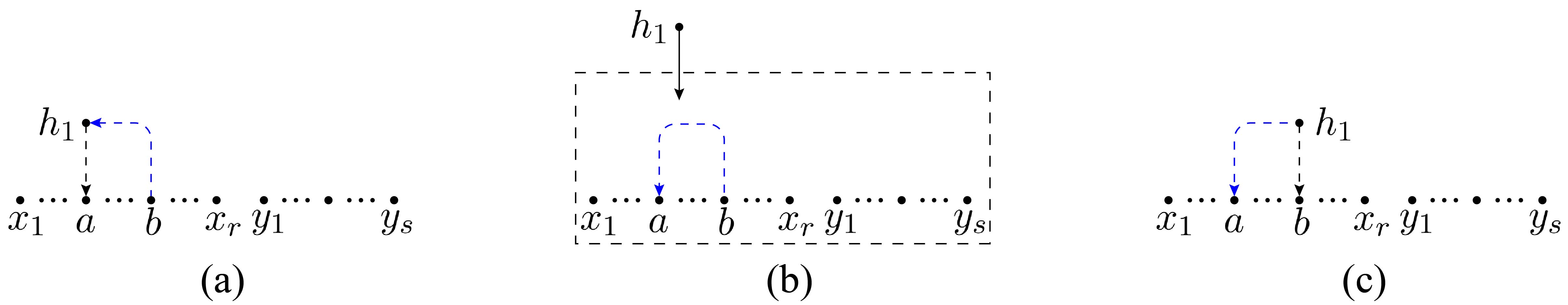
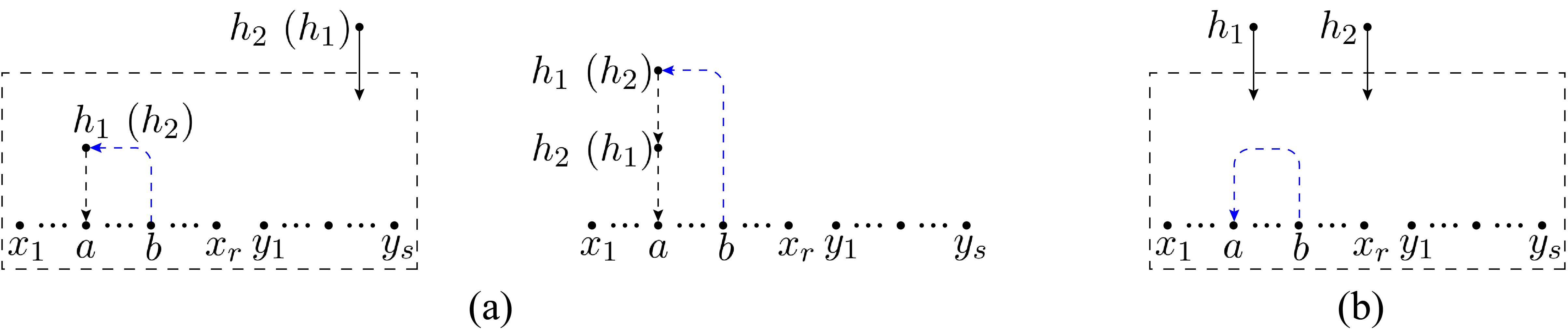
As shown by Fig. 16, there are three spanning forests (a), (f) and (h) for the amplitude with only one graviton , which correspond to the three cases that the graviton is (i) outside the bridge, (ii). on the LHS of the bridge and (iii) on the RHS of the bridge, respectively.
After transforming spanning forest (a) with transformation-3 and then the resulted graph (c) with transformation-1, graphs (d) and (e) are obtained. Graph (g) also comes from the transformation-3 of spanning forest (f). For graph (h), we apply transformation-2 to get graphs (i) and (j), and then apply transformation-2 to graph (j) to get graphs (l), (m), and (n). Since graphs (d) and (k) (graphs (g) and (m)) are the same except for the signs, after they cancel with each other out, the spanning forests for one-graviton amplitude only provide graphs (e), (l) and (n) with bridges formed by type-3 and type-4 edges. Therefore, the formula (2.1) and the formula (2.7) for -amplitude with one graviton are equivalent.
Appendix B The vanishing condition of
Now we consider a matrix on the RHS of (4.89), in which three columns have the same . Any minor corresponding to these three columns has the form:
| (B.4) |
where the form of depends on its position in the matrix (4.89)
| (B.9) |
Each row of determinant (B.4) has a common factor, , or that can be extracted out. Consequently, the determinant (B.4) is proportional to
| (B.13) |
Now we show that the determinant (B.13) vanishes in all possible situations:
- •
-
•
If (B.13) invloves one row or one column obtained from - or -blocks, this column or row can be considered as a column or row which comes from the block while replacing the momentum of the particle by the reference momentum . This has been seen in the MHV case in the previous subsection. Thus we only need to consider the remaining case that all rows and columns correspond to gluons and/or gravitons that come from block .
-
•
When all rows and columns refer to gluons and/or gravitons in original -block, the determinant (B.13) in general has the pattern
(B.17) which is further expanded as
(B.18) By the use of Schouten identity, one can straightforwardly verify that the above expression vanishes for either (i). the row labels , , and the column labels , , refer to distinct elements, or (ii). some of row indices are identical to some of the column indices (i.e. there exist zero entries which come from the diagonal entries of the original matrix ).
References
- (1) S. Stieberger and T. R. Taylor, New relations for Einstein-Yang-Mills amplitudes, Nucl. Phys. B913 (2016) 151–162, [arXiv:1606.09616].
- (2) D. Nandan, J. Plefka, O. Schlotterer, and C. Wen, Einstein-Yang-Mills from pure Yang-Mills amplitudes, JHEP 10 (2016) 070, [arXiv:1607.05701].
- (3) O. Schlotterer, Amplitude relations in heterotic string theory and Einstein-Yang-Mills, JHEP 11 (2016) 074, [arXiv:1608.00130].
- (4) C.-H. Fu, Y.-J. Du, R. Huang, and B. Feng, Expansion of Einstein-Yang-Mills Amplitude, JHEP 09 (2017) 021, [arXiv:1702.08158].
- (5) M. Chiodaroli, M. Gunaydin, H. Johansson, and R. Roiban, Explicit Formulae for Yang-Mills-Einstein Amplitudes from the Double Copy, JHEP 07 (2017) 002, [arXiv:1703.00421].
- (6) F. Teng and B. Feng, Expanding Einstein-Yang-Mills by Yang-Mills in CHY frame, JHEP 05 (2017) 075, [arXiv:1703.01269].
- (7) Y.-J. Du, B. Feng, and F. Teng, Expansion of All Multitrace Tree Level EYM Amplitudes, arXiv:1708.04514.
- (8) Z. Bern, J. J. M. Carrasco, and H. Johansson, New Relations for Gauge-Theory Amplitudes, Phys. Rev. D78 (2008) 085011, [arXiv:0805.3993].
- (9) Y.-J. Du and F. Teng, BCJ numerators from reduced Pfaffian, JHEP 04 (2017) 033, [arXiv:1703.05717].
- (10) Y.-J. Du and Y. Zhang, Gauge invariance induced relations and the equivalence between distinct approaches to NLSM amplitudes, JHEP 07 (2018) 177, [arXiv:1803.01701].
- (11) L. Hou and Y.-J. Du, A graphic approach to gauge invariance induced identity, JHEP 05 (2019) 012, [arXiv:1811.12653].
- (12) Y.-J. Du and L. Hou, A graphic approach to identities induced from multi-trace Einstein-Yang-Mills amplitudes, JHEP 05 (2020) 008, [arXiv:1910.04014].
- (13) K. Wu and Y.-J. Du, Off-shell extended graphic rule and the expansion of Berends-Giele currents in Yang-Mills theory, JHEP 01 (2022) 162, [arXiv:2109.14462].
- (14) Y.-J. Du and K. Wu, Note on graph-based BCJ relation for Berends-Giele currents, arXiv:2207.02374.
- (15) H. Tian, E. Gong, C. Xie, and Y.-J. Du, Evaluating EYM amplitudes in four dimensions by refined graphic expansion, JHEP 04 (2021) 150, [arXiv:2101.02962].
- (16) F. Porkert and O. Schlotterer, One-loop amplitudes in Einstein-Yang-Mills from forward limits, arXiv:2201.12072.
- (17) K. Zhou, Transmutation operators and expansions for -loop Feynman integrands, arXiv:2201.01552.
- (18) J. Faller and J. Plefka, Positive helicity Einstein-Yang-Mills amplitudes from the double copy method, Phys. Rev. D 99 (2019), no. 4 046008, [arXiv:1812.04053].
- (19) S. J. Parke and T. R. Taylor, An Amplitude for Gluon Scattering, Phys. Rev. Lett. 56 (1986) 2459.
- (20) D. Nguyen, M. Spradlin, A. Volovich, and C. Wen, The Tree Formula for MHV Graviton Amplitudes, JHEP 07 (2010) 045, [arXiv:0907.2276].
- (21) A. Hodges, A simple formula for gravitational MHV amplitudes, arXiv:1204.1930.
- (22) B. Feng and S. He, Graphs, determinants and gravity amplitudes, JHEP 10 (2012) 121, [arXiv:1207.3220].
- (23) Y.-J. Du, F. Teng, and Y.-S. Wu, Direct Evaluation of -point single-trace MHV amplitudes in 4d Einstein-Yang-Mills theory using the CHY Formalism, JHEP 09 (2016) 171, [arXiv:1608.00883].
- (24) F. Cachazo, S. He, and E. Y. Yuan, Einstein-Yang-Mills Scattering Amplitudes From Scattering Equations, JHEP 01 (2015) 121, [arXiv:1409.8256].
- (25) F. Cachazo, S. He, and E. Y. Yuan, Scattering equations and Kawai-Lewellen-Tye orthogonality, Phys. Rev. D90 (2014), no. 6 065001, [arXiv:1306.6575].
- (26) F. Cachazo, S. He, and E. Y. Yuan, Scattering of Massless Particles in Arbitrary Dimensions, Phys. Rev. Lett. 113 (2014), no. 17 171601, [arXiv:1307.2199].
- (27) F. Cachazo, S. He, and E. Y. Yuan, Scattering of Massless Particles: Scalars, Gluons and Gravitons, JHEP 07 (2014) 033, [arXiv:1309.0885].
- (28) F. Cachazo, S. He, and E. Y. Yuan, Scattering Equations and Matrices: From Einstein To Yang-Mills, DBI and NLSM, JHEP 07 (2015) 149, [arXiv:1412.3479].
- (29) Y.-j. Du, F. Teng, and Y.-s. Wu, CHY formula and MHV amplitudes, JHEP 05 (2016) 086, [arXiv:1603.08158].
- (30) S. Weinzierl, On the solutions of the scattering equations, JHEP 04 (2014) 092, [arXiv:1402.2516].
- (31) Y.-J. Du, F. Teng, and Y.-S. Wu, Characterizing the solutions to scattering equations that support tree-level Nk MHV gauge/gravity amplitudes, JHEP 11 (2016) 088, [arXiv:1608.06040].
- (32) D. Roberts, Mathematical Structure of Dual Amplitudes. PhD thesis, Durham University, 1972. Available at Durham E-Theses online.
- (33) D. Fairlie and D. Roberts, “Dual Models without Tachyons - a New Approach.” unpublished Durham preprint PRINT-72-2440, 1972.
- (34) D. B. Fairlie, A Coding of Real Null Four-Momenta into World-Sheet Co-ordinates, Adv. Math. Phys. 2009 (2009) 284689, [arXiv:0805.2263].
- (35) R. Monteiro and D. O’Connell, The Kinematic Algebras from the Scattering Equations, JHEP 03 (2014) 110, [arXiv:1311.1151].
- (36) Y. Geyer, A. E. Lipstein, and L. J. Mason, Ambitwistor Strings in Four Dimensions, Phys. Rev. Lett. 113 (2014), no. 8 081602, [arXiv:1404.6219].
- (37) L. Mason and D. Skinner, Ambitwistor strings and the scattering equations, JHEP 07 (2014) 048, [arXiv:1311.2564].
- (38) L. Dolan and P. Goddard, General Solution of the Scattering Equations, arXiv:1511.09441.
- (39) C. Cardona and C. Kalousios, Elimination and recursions in the scattering equations, Phys. Lett. B756 (2016) 180–187, [arXiv:1511.05915].
- (40) F. Cachazo and G. Zhang, Minimal Basis in Four Dimensions and Scalar Blocks, arXiv:1601.06305.
- (41) S. He, Z. Liu, and J.-B. Wu, Scattering Equations, Twistor-string Formulas and Double-soft Limits in Four Dimensions, JHEP 07 (2016) 060, [arXiv:1604.02834].
- (42) Z. Xu, D.-H. Zhang, and L. Chang, Helicity Amplitudes for Multiple Bremsstrahlung in Massless Nonabelian Gauge Theories, Nucl. Phys. B 291 (1987) 392–428.
- (43) E. Witten, Perturbative gauge theory as a string theory in twistor space, Commun. Math. Phys. 252 (2004) 189–258, [hep-th/0312171].
- (44) F. Cachazo, Resultants and Gravity Amplitudes, arXiv:1301.3970.
- (45) F. Cachazo and D. Skinner, Gravity from Rational Curves in Twistor Space, Phys. Rev. Lett. 110 (2013), no. 16 161301, [arXiv:1207.0741].
- (46) F. Cachazo, L. Mason, and D. Skinner, Gravity in Twistor Space and its Grassmannian Formulation, SIGMA 10 (2014) 051, [arXiv:1207.4712].