A Nonnested Augmented Subspace Method for Kohn-Sham Equation
Abstract
In this paper, a novel adaptive finite element method is proposed to solve the Kohn-Sham equation based on the moving mesh (nonnested mesh) adaptive technique and the augmented subspace method. Different from the classical self-consistent field iterative algorithm which requires to solve the Kohn-Sham equation directly in each adaptive finite element space, our algorithm transforms the Kohn-Sham equation into some linear boundary value problems of the same scale in each adaptive finite element space, and then the wavefunctions derived from the linear boundary value problems are corrected by solving a small-scale Kohn-Sham equation defined in a low-dimensional augmented subspace. Since the new algorithm avoids solving large-scale Kohn-Sham equation directly, a significant improvement for the solving efficiency can be obtained. In addition, the adaptive moving mesh technique is used to generate the nonnested adaptive mesh for the nonnested augmented subspace method according to the singularity of the approximate wavefunctions. The modified Hessian matrix of the approximate wavefunctions is used as the metric matrix to redistribute the mesh. Through the moving mesh adaptive technique, the redistributed mesh is almost optimal. A number of numerical experiments are carried out to verify the efficiency and the accuracy of the proposed algorithm.
Keywords. Density functional theory, Kohn-Sham equation, nonnested mesh, augmented subspace method.
AMS subject classifications. 65N30, 65N25, 65L15, 65B99.
1 Introduction
Density functional theory (DFT) is one of the major breakthroughs in quantum physics and quantum chemistry. In the framework of density functional theory, the many-body problem can be simplified as the motion of electrons without interaction in the effective potential field, which includes the Coulomb potential of the external potential field, the Hartree potential generated by the interaction between electrons, and the exchange-correlation potential for the nonclassical Coulomb interaction. For the exchange-correlation potential, it has always been a difficulty in density functional theory. At present, there is no exact analytical expression for the exchange-correlation potential. Generally, it is approximately described by the local density approximation (LDA), the local spin density approximation (LSDA) and the generalized gradient approximation (GGA), etc. The Kohn-Sham equation is one of the most important models in the calculation of electronic structure, which transforms the wavefunctions (in space) describing particle states into density function (in space), so as to reduce the degrees of freedom of equation and reduce the computational work of numerical simulation. The idea of Kohn-Sham equation can be traced back to Thomas-Fermi model in 1927. The model gave a primary description of the electronic structure of atoms. The strict theoretical analysis was described by Hohenberg and Kohn in [26], which proved the correctness and feasibility of using single electron orbit to replace the wavefunctions describing multiple electrons.
So far, lots of numerical methods for solving Kohn-Sham equation have been developed. For instance, plane-wave method [10, 35] is the most popular method in the computational quantum chemistry community. Since the basis function is independent from the ionic position, plane-wave method has advantage in calculating intermolecular force. Combined with the pseudopotential method, plane-wave method plays an important role in the study of the ground and excited states calculations, and geometry optimization of the electronic structures. Although the plane-wave method is the most popular one in the computational quantum chemistry community, it is inefficient in solving non-periodic systems like molecules, nano-clusters, or materials systems with defects, etc. Furthermore, the plane-wave method uses the global basis which significantly affect the scalability on parallel computing platforms. The atomic-orbital-type basis sets [21, 22] are also widely used for simulating materials systems such as molecules and clusters. However, they are well-suited only for isolated systems with special boundary conditions. It is difficult to develop a systematic basis-set for all materials systems. Thus over the past decades, more and more attentions are attracted to develop efficient and scalable grid-based methods such as the finite element method for electronic structure calculations. The advantages of grid-based methods include that it can use unstructured meshes and local basis sets, hence owing high scalability on parallel computing platforms. So far, the applications of the finite element method in solving Kohn-Sham equation have been studied systematically. We refer to [6, 8, 11, 33, 36, 39, 40, 42, 43, 47, 48, 49] and references therein for a comprehensive overview.
In this paper, we propose a nonnested augmented subspace method to solve the Kohn-Sham equation based on the moving mesh adaptive technique and the augmented subspace method. Since the Coulomb potential and Hartree potential have strong singularities, the adaptive mesh refinement is a competitive strategy to improve solving efficiency. Adaptive methods mainly include -adaptive method, -adaptive method and -adaptive method. The -adaptive method uses a posteriori error indicator for local refinement, -adaptive method uses higher-order polynomials on local mesh elements, -adaptive method (moving mesh method) uses control function or metric tensor (also known as metric matrix) for mesh redistribution. In this paper, we adopt the -adaptive method to generate a series of nonnested adaptive finite element spaces. The -adaptive method uses the control function or metric matrix to guide the mesh movement, which can improve the accuracy by moving the grid nodes to the area with large errors. This method can be traced back to Alexander’s work in [3], and then Miller’s work [37, 38] promoted the development of -adaptive method. In 2001, Li and Tang etc [31, 32] proposed the moving mesh method based on harmonic mapping. Later, Di and Li etc [18] applied the moving mesh method based on harmonic mapping to solve the incompressible Navier-Stokes equation. More results about moving mesh method can be found in [19, 20, 53, 54] and the references therein.
Another technique adopted in this paper is the multilevel correction method (augmented subspace method) [27, 34, 51, 52]. The traditional multilevel correction method can only be performed on the nested multilevel space sequence. In this paper, we develop a nonnested multilevel correction technique for Kohn-Sham equation on a nonnested mesh sequence generated by the moving mesh technique. Different from the classical self-consistent field iterative algorithm which requires to solve the Kohn- Sham equation directly in each adaptive finite element space, our algorithm transforms the Kohn-Sham equation into some linear boundary value problems of the same scale on each level of the adaptive refinement mesh sequence, and then the wavefunctions derived from the linear boundary value problems are corrected by solving a small-scale Kohn-Sham equation defined in a low-dimensional augmented subspace. Since the new algorithm avoids solving large-scale Kohm-Sham equation directly, a significant improvement for the efficiency can be obtained. In addition, the adaptive mesh is produced using the moving mesh technique according to the singularity of the wavefunctions, which can dramatically generate a high accuracy with less computational work. In our algorithm, the approximate wavefunctions are used as the adaptive function, and the modified Hessian matrix of the density function is used as the metric matrix to redistribute the mesh. Through the moving mesh adaptive technique, the redistributed mesh is almost optimal. By combining the moving mesh technique and the nonnested augmented subspace method, the solving efficiency for Kohn-Sham equation can be significantly improved.
The remainder of this paper is as follows. Section 2 introduces Kohn-Sham equation and its finite element discretization method. Section 3 introduces the nonnested augmented subspace method for Kohn-Sham equation by using the moving mesh technique and the multilevel correction method. In Section 4, we propose the convergence analysis and the estimate of computational work for the presented algorithm. In Section 5, a number of numerical examples are demonstrated to verify the efficiency and accuracy of the proposed method.
2 Finite element method for Kohn-Sham equation
To describe the Kohn-Sham equation and its finite element discretization, we first introduce some notation. Following [1], we use to denote Sobolev spaces, and use and to denote the associated norms and seminorms, respectively. In case , we denote and , where is in the sense of trace, and denote . For convenience, the symbols , and are used to represent , , and , respectively, where , , , and denote some mesh-independent constants. In this paper, is dropped from the subscript of the norm for simplicity.
Let be the Hilbert space with the inner product
| (2.1) |
where . For any and a subdomain , we define and
Let be a subspace of with orthonormality constraints:
| (2.2) |
where .
We consider a molecular system consisting of nuclei with charges , , and locations , , , respectively, and electrons in the non-relativistic and spin-unpolarized setting. The general form of Kohn-Sham energy functional can be demonstrated as follows
| (2.3) |
for . Here, is the Coulomb potential defined by , is the Hartree energy defined by
| (2.4) |
and is some real function over denoting the exchange-correlation energy.
The ground state of the system is obtained by solving the minimization problem:
| (2.5) |
and we refer to [10, 16] for the existence of a minimizer under some conditions.
The Euler-Lagrange equation corresponding to the minimization problem (2.5) is the well-known Kohn-Sham equation: Find such that
| (2.6) |
where is the Kohn-Sham Hamiltonian operator defined by
| (2.7) |
with , , and . The variational form of the Kohn-Sham equation can be described as follows: Find such that
| (2.8) |
Now, let us define the finite element discretization of (2.8). First we generate a shape regular decomposition of the computing domain . Then, based on the mesh , we construct the linear finite element space denoted by . Define . Then the discrete form of (2.8) can be described as follows: Find such that
| (2.9) |
with .
For simplicity and generality, some assumptions are given for the error analysis of the proposed algorithm in this paper. We would like to mention that the following assumptions are satisfied by many practical physical models. For detail of the assumptions, please refer to [9, 10, 14, 15].
-
•
Assumption A: for some , where denotes the following function set:
(2.10) with and , .
-
•
Assumption B: There exists a constant such that .
-
•
Assumption C: Let be a solution of (2.8). When the mesh size is small enough, the discrete solution satisfies the following estimate
(2.11) (2.12) where and
3 Nonnested augmented subspace method for Kohn-Sham equation
In this section, we design the nonnested augmented subspace method for Kohn-Sham equation based on the moving mesh adaptive technique and the augmented subspace method. In the first two subsections, we introduce some computing techniques including the solving process for exchange-correlation potential and Hartree potential, and the detailed process of moving mesh technique. Then next, we combine these techniques to generate the nonnested augmented subspace method for Kohn-Sham equation.
3.1 The calculation of exchange-correlation potential and Hartree potential
The Kohn-Sham equation contains two nonlinear terms: the Hartree potential and the exchange-correlation potential. In this subsection, we introduce the detailed form for exchange-correlation potential and the solving process for Hartree potential.
Since there is no exact expression for the exchange-correlation potential, we use the local density approximation (LDA) in our numerical simulations. The exchange-correlation potential can be treated as the variational derivative of the exchange-correlation energy to the density function . The exchange-correlation energy is divided into two parts: exchange energy and correlation energy , that is . For the exchange energy, we use the following approximate form given by Kohn and Sham in [30]:
| (3.1) |
with the exchange-correlation potential
| (3.2) |
For the relatively complex correlation energy and correlation potential, we use the expression proposed by Perdew and Zunger in [44]. The correlation energy per electron is:
The corresponding correlation potential is
| (3.3) |
with .
The ground state energy of the molecular system can be calculated through:
| (3.4) |
The last term accounts for the interactions between the nuclei:
| (3.5) |
Next, we introduce the solving process for Hartree potential , which is computed by solving the following Poisson equation:
| (3.6) |
Because the Hartree potential decays with the rate , where is the electron number, the simple use of zero Dirichlet boundary condition will introduce large truncation error on the boundary. To give the evaluation of the Hartree potential on the boundary, a multipole expansion approximation is employed for the boundary values. In our numerical simulations, the following approximation is used:
| (3.7) |
where
In the above expressions, is chosen as .
3.2 Moving mesh adaptive technique
The adaptive methods mainly include -adaptive method, -adaptive method and -adaptive method. The -adaptive method uses a posteriori error indicator for local refinement, -adaptive method uses higher-order polynomials on local mesh elements, -adaptive method uses control function or metric tensor (also known as metric matrix) for mesh redistribution. In this subsection, we introduce the detailed process for the -adaptive method which is used for mesh adaptive refinement in this paper.
The moving mesh adaptive (-adaptive) software packages mostly control mesh movement based on the control function or metric tensor. Some well-known finite element software packages such as AFEPack [18, 31, 32] are based on the control function. Other software packages such as BAMG [24], Mshmet and Mmg [17, 20] are based on metric tensor. Essentially, the control function and the measurement matrix are consistent. From mathematical point of view, they differ only by a constant factor. From the way of controlling the movement of the grid points, the control function is based on the error equal distribution principle, and the measurement matrix is based on the unit volume principle (BAMG) or the unit edge principle (mshmet and Mmg). Here, we use the three-dimensional anisotropic adaptive software Mshmet and Mmg3d (three-dimensional module in Mmg) based on the -unit side length principle, in which the measurement used is the correction of the Hessian matrix of the given adaptive function at the grid node . The detailed form is as follows:
| (3.8) |
where denotes the location of the grid node, denotes an orthogonal matrix composed of the orthogonal eigenfunctions of the Hessian matrix , is defined by
| (3.9) |
To guarantee the positive definite of the measurement matrix, is set to be
| (3.10) |
where is used to control the -interpolation error in the sense of -norm, denotes the eigenvalue of the Hessian matrix , and represent the upper limit of the longest edge scale and the lower limit of the shortest edge scale, respectively. In addition, the coefficient is selected based on the following error estimate (see [2]):
Lemma 3.1.
Let be a mesh element (d-dimensional simplex) of mesh , is a set of all edges on , and is a quadratic differentiable function. Then, we have the following interpolation error estimate
| (3.11) |
where
| (3.12) |
with .
The computation of the right term of (3.11) is nontrivial. Thus, we first assume that there exists a measurement , such that
| (3.13) |
To derive , it is sufficient to require that
| (3.14) |
By defining the measurement , and based on (3.14), we know the measurement satisfies the following unit edge length principle
| (3.15) |
That is, the length of side of element under is 1, which is denoted by
| (3.16) |
In the actual calculation, can be determined by (3.8)(3.10). In fact, in the software package Mshmet, we only need to adjust the parameters err, hmin, hmax to control the edge length of mesh elements. For more detailed introduction to the metric based adaptive mesh using the unit edge length principle, please refer to [2, 20]. For more discussion on metric matrices and control functions, please refer to [19, 53, 54].
Next, we introduce a fast interpolation algorithm between two nonnested meshes. Let and be two different computing domains, and be the corresponding mesh decompositions on these two domains, respectively. The two decompositions are nonnested. Then, we briefly introduce the fast interpolation algorithm proposed by the FreeFEM team to deal with nonnested meshes [23].
Let be the finite element space defined on and . For , the problem is to find such that:
| (3.17) |
A fast interpolation algorithm is proposed in [23] which is of complexity , where is the number of vertices of , is the number of vertices of . The detailed process is presented in Algorithm 1.
3.3 Nonnested augmented subspace method for Kohn-Sham equation
In this subsection, we introduce the nonnested augmented subspace algorithm for Kohn-Sham equation. To simplify the description, we define a nonlinear operator which is composed of the Kohn-Sham Hamiltonian operator and a positive constant:
| (3.18) |
where is a positive constant that can be used to guarantee the coercive property.
The essence of the nonnested augmented method is to transform the solution of the Kohn-Sham equation on the fine mesh into solving the linear boundary value problems of the same scale and solving a small-scale Kohn-Sham equation in a low-dimensional subspace. In order to describe the nonnested augmented subspace algorithm, we generate a coarse mesh and corresponding linear finite element space . The traditional multilevel correction method requires the multilevel finite element space sequence satisfies the nested relationship
| (3.19) |
The nonnested augmented subspace method presented in this paper does not require the mesh and finite element space to meet the above nested property, which guarantees that the augmented subspace method can be used in moving mesh sequence. In Algorithm 2, the flowchart of the moving mesh adaptive algorithm for the Kohn-Sham equation is given.
| (3.20) |
Next, we introduce the an augmented subspace method to solve the Kohn-Sham equation (3.20), which transforms the large-scale nonlinear eigenvalue problem into some linear boundary value problems of the same scale and small-scale Kohn-Sham equations defined in a low-dimensional augmented subspace. Through the augmented subspace method, the total computational work is asymptotically optimal since the dimension of the augmented subspace is small and fixed. The detailed process is described in Algorithm 3.
| (3.22) |
| (3.24) |
From Algorithm 3, we can find that the Kohn-Sham equation (3.24) is defined in a low-dimensional space , thus a small-scale linear eigenvalue problem is needed to be solved in each nonlinear iteration step, which requires little computational work. But the augmented subspace includes the basis functions derived from the fine mesh , so the matrices assembling should be performed on the fine mesh to keep the accuracy.
Next, we introduce the detailed process for solving the small-scale Kohn-Sham equation (3.24) in . For simplicity, we use , , to denote , , , respectively. Define and . Let be the basis functions for . When solving (3.24) by iteration method, a linear eigenvalue problem as follows is required to be solved in each iteration step:
| (3.25) |
where
| (3.26) |
with , , . Here, is the eigenvector to be solved in each iteration step, and , is the number of eigenpair to be solved. The mass matrix remains unchanged during the nonlinear iteration, which can be assembled once at the beginning of Algorithm 3. Hereafter, denotes the -inner product on the mesh .
For the matrices and , the involved basis functions are defined on the fine mesh . Thus, to keep the accuracy, these matrices assembling should be performed on the fine mesh . As we can see, the basis functions remain unchanged during the nonlinear iteration step, thus the matrices and also can be assembled once at the beginning of Algorithm 3.
It is noted that, based on the above discussion, the mass matrix only need to be assembled once at the beginning of the nonlinear iteration in Algorithm 3. No updates are required during the iteration.
Next, we discuss the stiffness matrix . Let us divide the stiffness matrix into linear and nonlinear parts. The linear part is defined by:
| (3.27) |
The nonlinear part consisting of the Hartree potential and exchange-correlation potential is defined by:
| (3.28) |
where and need to be updated in each nonlinear iteration because they depends on the density function that will be updated after each iteration. Let us define . Using the interpolation algorithm defined in Algorithm 1. The matrix involved in can be calculated in the following way
| (3.29) |
where denotes the interpolate operator from to based on Algorithm 1.
The remaining parts and can be calculated by:
| (3.30) |
and
| (3.31) |
Remark 3.1.
Based on the assembling process (3.25)(3.31), the main computational work is spent on (3.28) in each nonlinear iteration. Fortunately, the matrix assembling can be performed in parallel since there is no date transfer, and meanwhile the software package used in this paper has an excellent parallel ability [29, 41], thus we assemble the matrix using parallel computing technique.
3.4 Convergence analysis and computational work estimate
In this subsection, we give the convergence analysis and computational complexity estimate for Algorithms 2 and 3. First, we can obtain the following theorem to guarantee the well-posedness of the linear boundary value problems.
Theorem 3.1.
With sufficiently small mesh size, there exists a positive constant such that the following coercive property holds true
| (3.32) |
where
| (3.33) |
Proof.
For the Coulomb potential , using the following uncertainty principle lemma [45]:
| (3.34) |
we obtain
| (3.35) | |||||
For the Hartree potential, using (3.34) and Hölder inequality, we have
| (3.36) | |||||
For the exchange-correlation potential, we have
| (3.37) |
From Assumption A, we have . For the first part of (3.37), the following estimate holds
| (3.38) |
with and . Using Assumption B, we can further derive
| (3.39) | |||||
Inserting (3.39) into (3.37) and using Holder inequality, we can derive
| (3.40) |
where is the mesh-independent constant involved in embedding theorem , when .
Theorem 3.2.
Under Assumption A-C, the eigenpair approximation derived by by Algorithm 3 has following error estimates
| (3.42) |
| (3.43) |
where the projection operator is defined by: and
| (3.44) |
Proof.
From (2.8) and (3.44), the following equation holds true for :
| (3.45) |
Then from (3.22) and (3.45), we obtain
| (3.46) |
Now let us estimate the equation (3.46) termwise. We deduce from triangle inequality that
For the Hartree potential, using the uncertain principle lemma, the following inequalities hold
| (3.47) |
For any , based on Assumption B, the exchange-correlation potential can be estimated by
| (3.48) |
where with .
For the first part of (3.48), we have
| (3.49) |
For the second and third parts of (3.48), using the proof technique for (3.40), the following estimate holds
| (3.50) |
Using (3.48), (3.49) and (3.50), there holds
| (3.51) |
Taking in (3.46), due to Lemma 3.1, (3.47), (3.48) and (3.51), we derive
| (3.52) |
which yields
| (3.53) | |||||
Since is a subspace of , the Kohn-Sham equation (3.24) can be regarded as a subspace approximation for (2.9). From Assumption C and (3.53), we have
This is the desired result (3.42). The estimate (3.43) can be obtained by Assumption C, and the proof is completed. ∎
Theorem 3.2 shows that the augmented subspace method defined by Algorithm 3 can really improve the accuracy after each iteration, which is the base for designing the nonnested augmented subspace method for Kohn-Sham equation.
Next, we estimate the computational work of the nonnested augmented subspace method. In this paper, we use Mshmet and Mmg3d [17, 20] to realize the moving mesh process. Therefore, the unit mesh principle shall be met [17, 20]. That is, for any , there holds
| (3.54) |
where is the metric on the mesh element , is the union of the boundaries of . Based on the definition of and the unit mesh principle (3.54), we can change the length of each edge through adjusting the value of , which then leads to the following relationship for the number of degrees of freedom:
| (3.55) |
where denotes the coarsening rate between two consecutive meshes.
Let denote the computational work in the th finite element space, denote the computational work for solving the Kohn-Sham equation in the first adaptive spaces, denote the number of mesh levels, denote the nonlinear iteration times, denote the number of processes. We use parallel computing technique to assemble the matrix in step 3 of Algorithm 3, and the resultant algebraic system is solved by the parallel algebraic multigrid method. Thus the computational work for the linear boundary value problems is . For the small-scale nonlinear eigenvalue problem involved in step 4 of Algorithm 3, the matrices are assembled through parallel computing technique, and the small-scale algebraic eigenvalue problem is solved in serial computing with computational work . Then the total computational work in the th finite element space is
| (3.56) |
Theorem 3.3.
Proof.
Remark 3.2.
For complicated molecular system, the number of the desired eigenpairs and the number of nonlinear iteration times will be large. But fortunately, the software package FreeFEM [29] has a good scalability. Thus, when the number of processes is large, we can still derive an asymptotically optimal computational work estimate.
4 Numerical experiments
In this section, we provide four numerical examples to validate the efficiency of the proposed nonnested augmented subspace method in this paper. These numerical examples are implemented on the high performance computing platform LSSC-IV in the State Key Laboratory of Scientific and Engineering Computing, Chinese Academy of Sciences. Each computing node has two 18-core Intel Xeon Gold 6140 processors at 2.3 GHz and 192 GB memory. All the parallel solving processes in this paper use 72 cores. We adopt the open source finite element software package FreeFEM [23, 29] to do the numerical simulation. The anisotropic measurement is generated by the Meshmet of Hessian matrix based on adaptive function (density function), and the adaptive mesh is generated by the software package Mmg3d [17, 20]. The involved linear boundary value problems are solved by PETSc-GAMG [5], and the linear eigenvalue problems are solved by Krylov-Schur method [25] in SLEPc [46]. In all the numerical experiments, we set the threshold in Algorithm 2 to be , and set the positive constant in Algorithm 3 to be .
For the nonlinear eigenvalue problems, we use the Anderson mixing scheme to accelerate the convergence rate [4]. The detailed process can be described as follows: Let and represent the input and output electron densities of the -th self-consistent iteration. To input the -th self-consistent iteration, is computed as follows:
| (4.1) |
where
| (4.2) |
and the sum of the coefficients equals to one, i.e.,
| (4.3) |
According to (4.3), the equation (4.2) can be written as
| (4.4) |
Here the positive integer , and the depth of the mixing scheme is defined by depth, is a given weight value.
Denoting and . Based on (4.4), there holds
| (4.5) |
The coefficients are determined by minimizing , which amounts to solve the following equations:
| (4.6) |
In our numerical experiments, we choose the depth, the damping coefficient .
4.1 Kohn-Sham equation for Helium
In the first example, we solve the following Kohn-Sham equation for Helium:
| (4.7) |
where . In this example, the electron density . The exchange-correlation potential is chosen according to (3.2) and (3.3). The experimental value of non-relativistic ground state energy of Helium atom is -2.90372 hartree [50].
Here, we use three types of algorithms to solve the Kohn-Sham equation (4.7). The first one uses the self-consistent field iteration to solve (4.7) directly on the fixed structure mesh. The second one uses the self-consistent field iteration to solve (4.7) directly on the adaptive moving mesh (i.e. step 3 of Algorithm 2 is solved directly by the self-consistent field iteration). The third one uses the nonnested augmented subspace method to solve (4.7). In the moving mesh adaptive process, the metric matrix is given by the modified Hessian matrix (3.8) of . The tolerance in Algorithm 2 is set to be . The tolerance in Algorithm 3 is set to be .
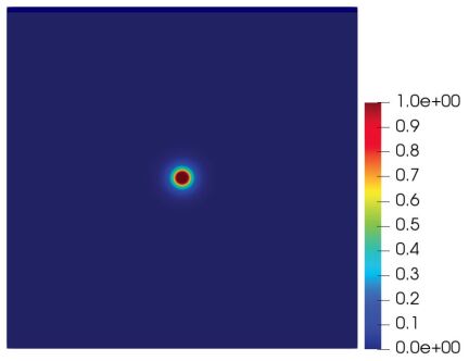
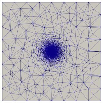
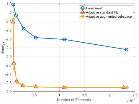
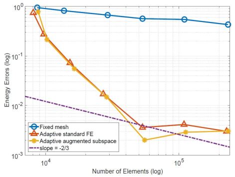
The density function and the adaptive mesh of the nonnested augmented subspace method are presented in Figure 1. The ground state energy and the corresponding error estimates derived by these three methods are presented in Figure 2. It can be seen from Figure 2 that the ground state energy of Helium atom first decreases quickly and then tends to be stable with the adaptive refinement of the mesh. Besides, we also can see that the adaptive iterative methods have a better accuracy than the finite element method with the uniform mesh.
4.2 Kohn-Sham equation for Hydrogen-Lithium
In the second example, we solve the following Kohn-Sham equation for Hydrogen-Lithium:
| (4.8) |
where . In this equation, the electron density , is the position of lithium atom and hydrogen atom and we take , . The exchange-correlation potential is chosen according to (3.2) and (3.3). The experimental value of non relativistic ground state energy of Hydrogen-Lithium molecular system is -8.070 hartree [12]. In this example, we set the tolerance in Algorithm 2 to be and tolerance in Algorithm 3 to be . We also use these three numerical methods as described in the first example to solve (4.8).
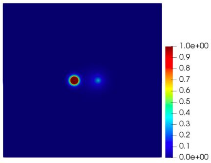
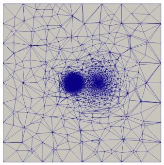
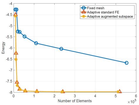
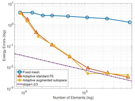
The density function and the adaptive mesh for Hydrogen-Lithium are presented in Figure 3. The ground state energy and the corresponding error estimates derived by these three methods are presented in Figure 4. It can be seen from Figure 4 that the ground state energy of Hydrogen-Lithium decreases quickly to a stable constant with the adaptive refinement of the mesh. Besides, we also can see that the adaptive iterative methods have a better accuracy than the finite element method with uniform mesh. At the same time, it can be seen that the convergence rate of Algorithm 3 tends to with mesh refinement.
| Elements (Direct method) | 9008 | 11463 | 15943 | 29015 | 57078 | 113729 | 240435 | 518786 |
|---|---|---|---|---|---|---|---|---|
| Time (Direct method) | 7.024 | 10.231 | 14.188 | 18.587 | 23.694 | 32.339 | 46.215 | 74.595 |
| Elements (Algorithm 3) | 8819 | 11240 | 17235 | 31297 | 55690 | 113168 | 236780 | 510949 |
| Time (Algorithm 3) | 8.642 | 11.176 | 15.370 | 19.260 | 23.340 | 30.560 | 38.086 | 49.016 |
In Table 1, we present the computational time of the nonnested augmented subspace method and the direct adaptive finite element method (i.e. solve the Kohn-Sham equation directly using the moving mesh adaptive technique). It can be seen that the nonnested augmented subspace method is more efficient when the number of mesh elements reaches 55690 or more, and the advantage is more obvious with the increase of the number of mesh elements.
4.3 Kohn-Sham equation for Methane
In the third example, we consider the Kohm-Sham equation for Methane. To show the efficiency of the nonnested augmented subspace method intuitively, we also use these three methods described in Example 4.1 to solve the Methane molecules. The computational domain is set to be , and the atomic positions of Methane are shown in Table 2.
| Atom | x | y | z | Nuclear charge |
|---|---|---|---|---|
| 0.0000 | 0.0000 | 0.0000 | 6 | |
| 1.3092 | 1.3092 | 1.3092 | 1 | |
| -1.3092 | -1.3092 | 1.3092 | 1 | |
| 1.3092 | -1.3092 | -1.3092 | 1 | |
| -1.3092 | 1.3092 | -1.3092 | 1 |
For a full potential calculation, there are total ten electrons. Since we don’t consider spin polarisation, five eigenpairs need to be calculated. The tolerance setting in Algorithms 2 and 3 is the same as that of Example 4.1. The reference value of non relativistic ground state energy of methane molecule is set to be -40.41 hartree [28].
Figure 5 shows the electron density distribution and adaptive mesh of Methane molecule. Figure 6 shows the change curve of ground state energy and the corresponding error estimates for Methane molecule with the increasement of the number of mesh elements.
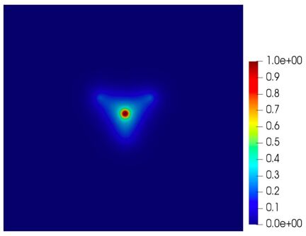
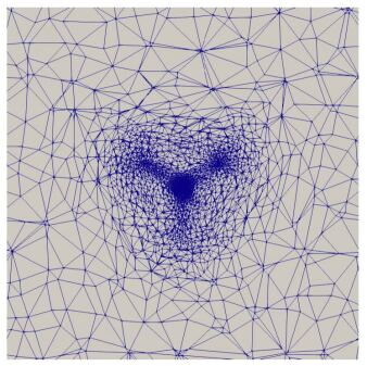
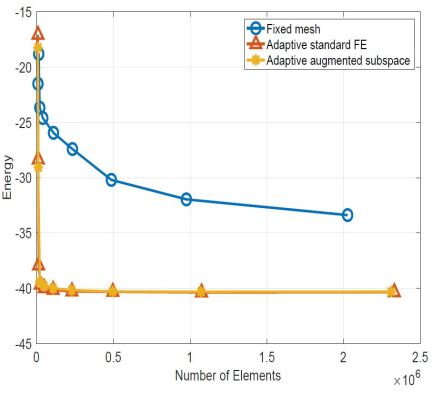
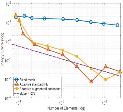
Table 3 shows the computational time of the nonnested augmented subspace method and the direct adaptive finite element method. It can be seen that when the number of mesh elements reaches 499064, the nonnested augmented subspace method has an advantages in solving efficiency over the direct adaptive finite element method.
| Elements (Direct method) | 10208 | 11496 | 22267 | 45982 | 102415 | 225074 | 492919 | 1072524 | 2329210 |
|---|---|---|---|---|---|---|---|---|---|
| Time (Direct method) | 10.904 | 15.141 | 20.737 | 29.902 | 42.412 | 68.716 | 140.839 | 312.876 | 756.633 |
| Elements (Algorithm 3) | 10545 | 10599 | 22682 | 51646 | 108014 | 230730 | 499064 | 1083722 | 2342607 |
| Time (Algorithm 3) | 10.762 | 14.027 | 19.386 | 30.579 | 53.005 | 70.812 | 86.976 | 149.184 | 209.735 |
4.4 Kohn-Sham equation for Benzene
In the last example, we consider the Kohn-Sham equation for the Benzene molecule. The computational domain is taken as , and the atomic positions of Methane are shown in Table 4.
| Atom | x | y | z | Nuclear charge |
|---|---|---|---|---|
| 0.0000 | 1.3970 | 0.0000 | 6 | |
| 1.2098 | 0.6985 | 0.0000 | 6 | |
| 1.2098 | -0.6985 | 0.0000 | 6 | |
| 0.0000 | -1.3970 | 0.0000 | 6 | |
| -1.2098 | -0.6985 | 0.0000 | 6 | |
| -1.2098 | 0.6985 | 0.0000 | 6 | |
| 0.0000 | 2.4810 | 0.0000 | 1 | |
| 2.1486 | 1.2405 | 0.0000 | 1 | |
| 2.1486 | -1.2405 | 0.0000 | 1 | |
| 0.0000 | -2.4810 | 0.0000 | 1 | |
| -2.1486 | -1.2405 | 0.0000 | 1 | |
| -2.1486 | 1.2405 | 0.0000 | 1 |
For a full potential calculation, there are total 42 electrons. Since we don’t consider spin polarisation, 21 eigenpairs need to be calculated. The tolerance setting in Algorithms 2 and 3 is the same as that of Example 4.1. The reference value of non relativistic ground state energy of methane molecule is set to be -231.78 hartree [28].
| Elements (Direct method) | 8946 | 13095 | 21675 | 58635 | 198145 | 535501 | 1245081 | 2789529 |
|---|---|---|---|---|---|---|---|---|
| Time (Direct method) | 19.079 | 28.454 | 40.958 | 63.495 | 109.606 | 223.390 | 470.353 | 1027.426 |
| Elements (Algorithm 3) | 8897 | 12505 | 20535 | 62348 | 207362 | 550236 | 1262297 | 2796022 |
| Time (Algorithm 3) | 14.235 | 21.239 | 35.367 | 62.337 | 79.789 | 133.229 | 187.119 | 294.440 |
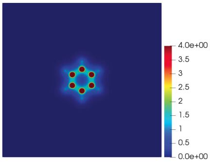
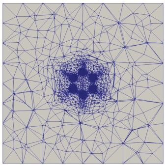
Three numerical methods described in Example 4.1 are tested in this example. Figure 7 shows the electron density and adaptive mesh of the nonnested augmented subspace method. It can be seen from Figure 7 that the mesh nodes gather in the region with singular electron density (near the atomic centers), while in the region far away from the atomic centers, the mesh node distribution is sparse, which is consistent with the distribution of electron density function.
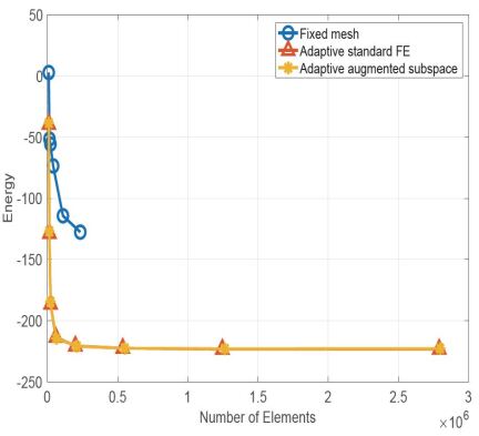
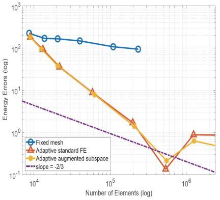
Figure 8 shows the decline curve of ground state energy and corresponding error estimates with mesh adaptive movement. From Figure 8, we can see that compared with the moving mesh adaptive method (red line and yellow line), the finite element method performed on the fixed structural mesh (blue line) derives a slower convergence rate. Moreover, when the number of mesh elements reaches 233280, the nonlinear iteration on fixed structure mesh still does not converge even if the Anderson acceleration technology is adopted.
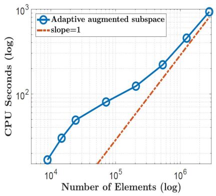
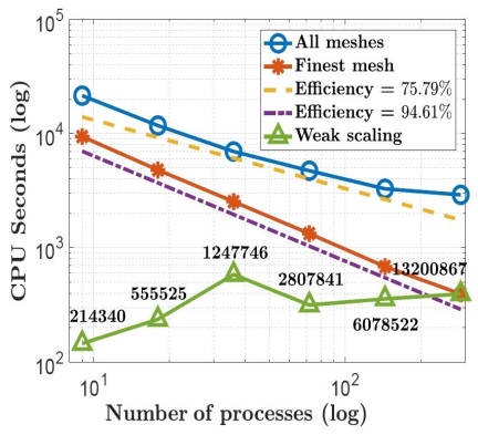
Table 5 compares the computational time of the nonnested augmented subspace method and the direct adaptive finite element method. It can be seen that when the number of mesh elements reaches 207362, the nonnested augmented subspace method has advantage in solving efficiency over the direct adaptive finite element method.
In addition, we also present the computational time of the nonnested augmented subspace method for Benzene in Figure 9 to test its linear complexity and the parallel scalability. Figure 9 shows that when the number of mesh elements reaches 500000, the nonnested augmented subspace method has a linear computational complexity with the increase of the number of mesh elements. The strong scalability and weak scalability is also presented in Figure 9. In Figure 9, the label “All meshes” (blue line) represents the total computational time from the coarsest mesh to the finest mesh. The labeled “finest mesh” (red line) represents only the computational time in the finest mesh, The green line is the result of weak scalability, and 9, 18, 36, 72, 144 and 288 processes are used, respectively. From Figure 9, we can find that the nonnested augmented subspace method has a good scalability.
5 Concluding remarks
In this paper, a nonnested augmented subspace method is proposed to solve the Kohn-Sham equation based on the moving mesh adaptive technique and augmented subspace method. Because the moving mesh adaptive technology is used to generate nonnested mesh sequence, the redistributed mesh is almost optimal. In the solving process, we transform the classical nonlinear eigenvalue problem on a fine mesh into a series of linear boundary value problems of the same scale on the adaptive mesh sequence, and subsequently correct the approximate solutions by solving the small-scale nonlinear eigenvalue problems in a special low-dimensional augmented subspace. Since solving large-scale nonlinear eigenvalue problem is avoided which is time-consuming, the total solving efficiency can be greatly improved. Some numerical experiments are also presented to verify the computational efficiency and energy accuracy of the algorithm proposed in this paper.
6 Acknowledgement
This research is supported partly by National Key R&D Program of China 2019YFA0709600, 2019YFA0709601, National Natural Science Foundations of China (Grant Nos. 11922120, 11871489 and 11771434), FDCT of Macao SAR (0082/2020/A2), MYRG of University of Macau (MYRG2020-00265-FST), the National Center for Mathematics and Interdisciplinary Science, CAS, Beijing Municipal Natural Science Foundation (Grant No. 1232001), and the General projects of science and technology plan of Beijing Municipal Education Commission (Grant No. KM202110005011).
References
- [1] R. A. Adams, Sobolev spaces, Academic Press, New York, 1975.
- [2] F. Alauzet and P.J. Frey, Estimateur d’erreur géométrique et métriques anisotropes pour l’adaptation de maillage. partie i : aspects théoriques, Rapport de recherche RR-4759, INRIA, 2003.
- [3] R. Alexander, P. Manselli and K. Miller, Moving finite elements for the Stefan problem in two dimensions, Ren. Accad., 1979, Naz. Lincei (Rome) LXVII:57–61.
- [4] D. Anderson, Iterative procedures for nonlinear integral equations, J. Assoc. Comput. Mach., 12 (1965), 547–560.
- [5] S. Balay, S. Abhyankar, M. Adams, et al., PETSc users manual, Technical Report ANL-95/11- Revision 3.13, 2020.
- [6] G. Bao, G. Hu and D. Liu, Numerical solution of the Kohn-Sham equation by finite element methods with an adaptive mesh redistribution technique, J. Sci. Comput., 55(2) (2012), 372–391.
- [7] T. L. Beck, Real-space mesh techniques in density functional theory, Rev. Modern Phys., 72 (2000), 1041–1080.
- [8] E. J. Bylaska, M. Host and J. H. Weare, Adaptive finite element method for solving the exact Kohn-Sham equation of density functional theory, J. Chem. Theory Comput., 5 (2009), 937–948.
- [9] E. Cancès, R. Chakir and Y. Maday, Numerical analysis of nonlinear eigenvalue problems, J. Sci. Comput., 45(1–3) (2010), 90–117.
- [10] E. Cancès, R. Chakir and Y. Maday, Numerical analysis of the planewave discretization of some orbital-free and Kohn-Sham models, ESAIM Math. Model. Numer. Anal., 46 (2012), 341–388.
- [11] A. Castro, H. Appel, M. Oliveira, C. A. Rozzi, X. Andrade, F. Lorenzen, M. A. L. Marques, E. K. U. Gross, A. Rubio, Octopus: A tool for the application of time-dependent density functional theory, Phys. Status Solidi B, 243 (2006), 2465–2488.
- [12] W. Cencek and J. Rychlewski, Benchmark calculations for and LiH molecules using explicitly correlated Gaussian functions, Chem. Phys. Lett., 320 (2000), 549–552.
- [13] J. R. Chelikowsky, N. Troullier and Y. Saad, Finite-difference pseudopotential method: Electronic structure calculations without a basis, Phys. Rev. Lett., 72 (1994), 1240–1243.
- [14] H. Chen, X. Dai, X. Gong, L. He, Z. Yang and A. Zhou, Adaptive finite element approximations for Kohn-Sham models, Multi. Model. Simul., 12(4) (2014), 1828–1869.
- [15] H. Chen, L. He and A. Zhou, Finite element approximations of nonlinear eigenvalue problems in quantum physics, Comput. Methods Appl. Mech. Engrg., 200(21) (2011), 1846–1865.
- [16] H. Chen, X. Gong, L. He, Z. Yang and A. Zhou, Numerical analysis of finite dimensional approximations of Kohn-Sham models, Adv. Comput. Math., 38 (2013), 225–256.
- [17] C. Dapogny, C. Dobrzynski and P.J. Frey, Three-dimensional adaptive domain remeshing, implicit domain meshing, and applications to free and moving boundary problems, J. Comput. Phys., 262 (2014), 358–378.
- [18] Y. Di, R. Li, T. Tang, et al., Moving mesh finite element method for the incompressible Navier-Stokes equations, SIAM J. Sci. Comput., 26(3) (2005), 1036–1056.
- [19] Y. Di, H. Xie and X. Yin, Anisotropic meshes and stabilization parameter design of linear SUPG method for 2D convection-dominated convection-diffusion equations, J. Sci. Comput., 76(1) (2018), 48–68.
- [20] P.J. Frey and F. Alauzet, Anisotropic mesh adaptation for CFD computations, Comput. Methods Appl. Mech. Engrg, 194 (2005), 5068–5682.
- [21] W. J. Hehre, R. F. Stewart and J. A. Pople, Self-consistent molecular-orbital methods. I. Use of Gaussian expansions of Slater-type atomic orbitals, J. Chem. Phys., 51 (1969), 2657–2664.
- [22] F. Jensen, Introduction to Computational Chemistry, Wiley Publishers, 1999.
- [23] F. Hecht, FreeFEM documentation release 4.6, 2020, https://doc.freefem.org/pdf/ FreeFEM-documentation.pdf.
- [24] F. Hecht, Bidimensional anisotropic mesh generator. Technical report, INRIA, Roc-quencourt, 1997. Sourcecode: http://www-rocq1.inria.fr/gamma/cdrom/www/bamg/eng.htm.
- [25] V. Hernandez, J.E. Roman, A. Tomas, et al., Krylov-Schur methods in SLEPc, SLEPc Technical Report STR-7, 2007. http://slepc.upv.es.
- [26] P. Hohenberg and W. Kohn, Inhomogeneous electron gas, Phys. Rev., 136 (1964), B864–B871.
- [27] S. Jia, H. Xie, M. Xie and F. Xu, A full multigrid method for nonlinear eigenvalue problems, Science China: Mathematics, 59 (2016), 2037–2048.
- [28] R. Johnson, Nist computational chemistry comparison and benchmark database, 2011, http://cccbdb. nist.gov.
- [29] P. Jolivet, F. Hecht, F. Nataf, et al., Scalable domain decomposition preconditioners for heterogeneous elliptic problems, Proceedings of the 2013 ACM/IEEE conference on Supercomputing. SC13. Best paper finalist. ACM, 80 (2013), 1–11.
- [30] W. Kohn and L. Sham, Self-consistent equations including exchange and correlation effects, Phys. Rev. A, 140 (1965), 1133–1138.
- [31] R. Li, T. Tang and P.W. Zhang, Moving mesh methods in multiple dimensions based on harmonic maps, J. Comput. Phys., 170 (2001), 562–588.
- [32] R. Li, T. Tang and P.W. Zhang, A moving mesh finite element algorithm for singular problems in two and three space dimensions, J. Comput. Phys., 177 (2002), 365–393.
- [33] L. Lin, J. Lu, L. Ying and W. E, Adaptive local basis set for Kohn-Sham density functional theory in a discontinuous Galerkin framework I: Total energy calculation, J. Comput. Phys., 231 (2012), 2140–2154.
- [34] Q. Lin and H. Xie, A multi-level correction scheme for eigenvalue problems, Math. Comp., 84(291) (2015), 71–88.
- [35] B. Liu, H. Chen, G. Dusson, J. Fang and X. Gao, An adaptive planewave method for electronic structure calculations, 2021, arXiv:2012.14806v2.
- [36] A. Masud and R. Kannan, B-splines and NURBS based finite element methods for Kohn-Sham equations, Comput. Methods Appl. Mech. Engrg., 241-244 (2012), 112–127.
- [37] K. Miller and R.N. Miller, Moving finite element methods I, SIAM J. Numer. Anal., 18 (1981) 1019–1032.
- [38] K. Miller, Moving finite element methods II, SIAM J. Numer. Anal., 18 (1981), 1033–1057.
- [39] N. A. Modine, G. Zumbach and E. Kaxiras, Adaptive-coordinate real-space electronic-structure calculations for atoms, molecules and solids, Phys. Rev. B, 55 (1997), 289–301.
- [40] P. Motamarri, M. Nowak, K. Leiter, J. Knap and V. Gavini, Higher-order adaptive finite-element methods for Kohn-Sham density functional theory, J. Comput. Phys., 253 (2013), 308–343.
- [41] J. Moulin, P. Jolivet and O. Marquet, Augmented Lagrangian preconditioner for large-scale hydrodynamic stability analysis, Comput. Methods Appl. Mech. Engrg., 351 (2019), 718–743.
- [42] J. E. Pask, B. M. Klein, P. A. Sterne and C. Y. Fong, Finite element methods in electronic-structure theory, Comput. Phys. Comm., 135 (2001), 1–34.
- [43] J. E. Pask and P. A. Sterne, Finite element methods in ab initio electronic structure calculations, Model. Simul. Mater. Sci. Eng., 13 (2005), R71–R96.
- [44] J. Perdew, A. Zunger, Self-interaction correction to density-functional approximation for many-electron systems, Phys. Rev., 23 (1981), 5048–5079.
- [45] M. Reed and B. Simon, Methods of Modern Mathematical Physics, Academic Press, New York, 1975.
- [46] J.E. Roman, C. Campos, E. Romero, et al., Krylov-Schur methods in SLEPc, Technical Report DSIC-II/24/02, 2020. http://slepc.upv.es.
- [47] V. Schauer and C. Linder, All-electron Kohn-Sham density functional theory on hierarchic finite element spaces, J. Comput. Phys., 250 (2013), 644–664.
- [48] C. K. Skylaris, P. D. Haynes, A. A. Mostofi and M. C. Payne, Introducing ONETEP: Linear-scaling density functional simulations on parallel computers, J. Chem. Phys., 122 (2005), 084119.
- [49] P. Suryanarayana, V. Gavini, T. Blesgen, K. Bhattacharya and M. Ortiz, Non-periodic finite-element formulation of Kohn-Sham density functional theory, J. Mech. Phys. Solids, 58 (2010), 256–280.
- [50] A. Veillard and E. Clementi, Correlation energy in atomic systems. V. Degeneracy effects for the secondrow atoms, J. Chem. Phys., 49 (1968), 2415–2421.
- [51] H. Xie, A multigrid method for eigenvalue problem, J. Comput. Phys., 274 (2014), 550–561.
- [52] H. Xie, A multigrid method for nonlinear eigenvalue problems, Science China: Mathematics (Chinese), 45(8) (2015), 1193–1204.
- [53] H. Xie and X. Yin, Metric tensors for the interpolation error and its gradient in norm, J. Comput. Phys., 256 (2014), 543–562.
- [54] W.Z. Huang and R.D. Russell, Adaptive moving mesh methods, Springer, New York, 2011.