This paper was converted on www.awesomepapers.org from LaTeX by an anonymous user.
Want to know more? Visit the Converter page.

A nonlinear semigroup approach to Hamilton-Jacobi equations–revisited

Panrui Ni    Lin Wang
Abstract

We consider the Hamilton-Jacobi equation

H(x,Du)+λ(x)u=c,xM,{H}(x,Du)+\lambda(x)u=c,\quad x\in M,

where MM is a connected, closed and smooth Riemannian manifold. The functions H(x,p){H}(x,p) and λ(x)\lambda(x) are continuous. H(x,p){H}(x,p) is convex, coercive with respect to pp, and λ(x)\lambda(x) changes the signs. The first breakthrough to this model was achieved by Jin-Yan-Zhao [11] under the Tonelli conditions. In this paper, we consider more detailed structure of the viscosity solution set and large time behavior of the viscosity solution on the Cauchy problem.

Keywords. Hamilton-Jacobi equations, viscosity solutions, weak KAM theory

Panrui Ni: Shanghai Center for Mathematical Sciences, Fudan University, Shanghai 200433, China; e-mail: [email protected]
      Lin Wang: School of Mathematics and Statistics, Beijing Institute of Technology, Beijing 100081, China; e-mail: [email protected]
Mathematics Subject Classification (2020): 37J50; 35F21; 35D40

1 Introduction and main results

Inspired by Aubry-Mather theory and weak KAM theory for classical Hamiltonian systems, an action minimizing method for contact Hamiltonian systems was developed in a series of papers [16, 17, 18, 19, 20]. Let H:TM×H:T^{*}M\times\mathbb{R}\to\mathbb{R} be a contact Hamiltonian. It turns out that the dependence of HH on the contact variable uu plays a crucial role in exploiting the dynamics generated by HH. By using previous dynamical approaches, some progress on viscosity solutions of Hamilton-Jacobi (HJ) equations have been achieved [16, 18, 20]. In particular, the structure of the set of solutions can be sketched if HH is uniformly Lipschitz in uu based on the works mentioned before. Shortly after [18] occurred, [12] generalized the results to ergodic problems by using PDE approachs. More recently, for a class of HJ equations with non-monotone dependence on uu, the first breakthrough was achieved by Jin-Yan-Zhao [11] under the Tonelli conditions. In that work, they provided a description of the solution set of the stationary equation (formulated as (E0) below) and revealed a bifurcation phenomenon with respect to the value cc in the right hand side, which opened a way to exploit further properties of viscosity solutions beyond well-posedness for HJ equations with non-monotone dependence on uu. The main results in this paper are motivated by [11].

Let us consider the stationary equation:

H(x,Du)+λ(x)u=c,xM.{H}(x,Du)+\lambda(x)u=c,\quad x\in M. (E0)

Throughout this paper, we assume MM is a closed, connected and smooth Riemannian manifold. DD denotes the spacial gradient with respect to xMx\in M. Denote by TMTM and TMT^{*}M the tangent bundle and cotangent bundle of MM respectively. Let H:TMH:T^{*}M\rightarrow\mathbb{R} satisfy

  • (C):

    H(x,p)H(x,p) is continuous;

  • (CON):

    H(x,p)H(x,p) is convex in pp, for any xMx\in M;

  • (CER):

    H(x,p)H(x,p) is coercive in pp, i.e. limpx+H(x,p)=+\lim_{\|p\|_{x}\rightarrow+\infty}H(x,p)=+\infty, where x\|\cdot\|_{x} denotes the norms induced by gg on both TMTM and TMT^{*}M.

Correspondingly, one has the Lagrangian associated to HH:

L(x,x˙):=suppTxM{x˙,pxH(x,p)},L(x,\dot{x}):=\sup_{p\in T^{*}_{x}M}\{\langle\dot{x},p\rangle_{x}-H(x,p)\},

where ,x\langle\cdot,\cdot\rangle_{x} represents the canonical pairing between TxMT_{x}M and TxMT^{*}_{x}M. The Lagrangian L(x,x˙)L(x,\dot{x}) satisfies the following properties:

  • (LSC):

    L(x,x˙)L(x,\dot{x}) is lower semicontinous in x˙\dot{x}, and continuous on the interior of its domain dom(L):={(x,x˙)TM:L(x,x˙)<+}\textrm{dom}(L):=\{(x,\dot{x})\in TM:\ L(x,\dot{x})<+\infty\};

  • (CON):

    L(x,x˙)L(x,\dot{x}) is convex in x˙\dot{x}, for any xMx\in M.

We also assume λ(x)\lambda(x) is continuous and satisfies

  • (±\pm):

    there exist x1,x2Mx_{1},x_{2}\in M such that λ(x1)>0\lambda(x_{1})>0 and λ(x2)<0\lambda(x_{2})<0.

Throughout this paper, we define

λ0:=λ(x)>0,\lambda_{0}:=\|\lambda(x)\|_{\infty}>0, (1.1)

where \|\cdot\|_{\infty} stands for the supremum norm of the functions on their domains. From an economical point of view, the assumption (±\pm) may be corresponding to a model with fluctuating interest rates. To be more precise, the rates depend on the space variable and admit values above and below zero at some places. From a theoretical point of view, it is a toy model of the HJ equations with non-monotone dependence on uu. Based on this model, we revealed some different phenomena from the cases with monotone dependence on uu can be revealed.

Remark 1.1.

The model (E0) has been considered in [21]. In that paper, the function λ(x)\lambda(x) is non-negative and positive on the projected Aubry set of H(x,p)H(x,p). In this case, the solution of (E0) is unique. The asymptotic behavior of the solution of (E0) is also studied in [21] when λ00\lambda_{0}\to 0. When λ00\lambda_{0}\to 0 and the assumption (±\pm) holds, the family of solutions of (E0) may diverge, one can refer to [13] for an example.

In [14], the well-posedness of the Lax-Oleinik semigroup was verified for contact HJ equations under very mild conditions. By virtue of that, we generalize the results in [11] to the cases from the Tonelli conditions to the assumptions (C), (CON) and (CER) above. Henceforth, for simplicity of notation, we omit the word “viscosity”, if it is not necessary to be mentioned.

Proposition 1.2 (Generalization of [11]).

Let

c0:=infuC(M)supxM{H(x,Du)+λ(x)u}.c_{0}:=\inf_{u\in C^{\infty}(M)}\sup_{x\in M}\bigg{\{}H(x,Du)+\lambda(x)u\bigg{\}}.

Then c0c_{0} is finite. Given cc0c\geq c_{0}, the W1,\|\cdot\|_{W^{1,\infty}}-norm of all subsolutions of (E0) is bounded. Moreover,

  • (1)

    (E0) has a solution if and only if cc0c\geq c_{0};

  • (2)

    if c>c0c>c_{0}, then (E0) has at least two solutions.

The definition of c0c_{0} is inspired by [5]. In light of that, c0c_{0} is called the critical value. Now we consider the most general case

H(x,u(x),Du(x))=c,xM,H(x,u(x),Du(x))=c,\quad x\in M,

where the Hamiltonian H(x,u,p)H(x,u,p) is continuous, superlinear in pp and uniformly Lipschitz in uu. It was pointed out in [12] that there is a constant cc\in\mathbb{R} such that the above equation has viscosity solutions. Here we give some examples on the set \mathfrak{C} of all such cc’s, which reveals the essential difference between the monotone cases and the non-monotone cases:

  • for classical Tonelli Hamiltonian H(x,p)H(x,p), the set ={c0}\mathfrak{C}=\{c_{0}\}. The number c0c_{0} is called the effective Hamiltonian or the Mañé critical value;

  • for the discounted Hamilton-Jacobi equation, i.e., the Hamiltonian is of the form λu+H(x,p)\lambda u+H(x,p) with λ>0\lambda>0, the set =\mathfrak{C}=\mathbb{R}, see for example [6];

  • for the model (E0) considered here, the set =[c0,+)\mathfrak{C}=[c_{0},+\infty). Here we note that the non-emptiness of \mathfrak{C} is proved under (CER) instead of H(x,p)H(x,p) is superlinear in pp. In view of the existence result in [12], it means Proposition 1.2 is a non-trivial generalization of [11];

  • for the Hamiltonian periodically depending on uu, i.e., H(x,u+1,p)H(x,u,p)H(x,u+1,p)\equiv H(x,u,p), the set \mathfrak{C} is a bounded closed interval, see [15].

Different from the Tonelli case considered in [11], some new ingredients are needed for a priori estimates of subsolutions under the assumptions (C), (CON) and (CER). Those estimates will be provided in Section 3. The remaining parts of the proof of Proposition 1.2 are similar to the one in [11]. We postpone it to Appendix A.3 for consistency.

Motivated by Proposition 1.2, we are devoted to exploiting more detailed information of this model. First of all, we obtain

Theorem 1.

Let cc0c\geq c_{0}. There exist the maximal element umaxu_{\max} and the minimal element uminu_{\min} in the set of solutions of (E0).

Remark 1.3.

The viscosity solutions are equivalent to backward weak KAM solutions in our settings (see [14, Proposition D.4]). In terms of the correspondence between backward and forward weak KAM solutions (see Proposition 2.7 below), it follows from Theorem 1 that there exist the maximal and minimal forward weak KAM solutions of (E0). We denote umin+u^{+}_{\min} (resp. umax+u^{+}_{\max}) the minimal (resp. maximal) froward weak KAM solution of (E0). By Proposition 2.8(3)(4), there hold
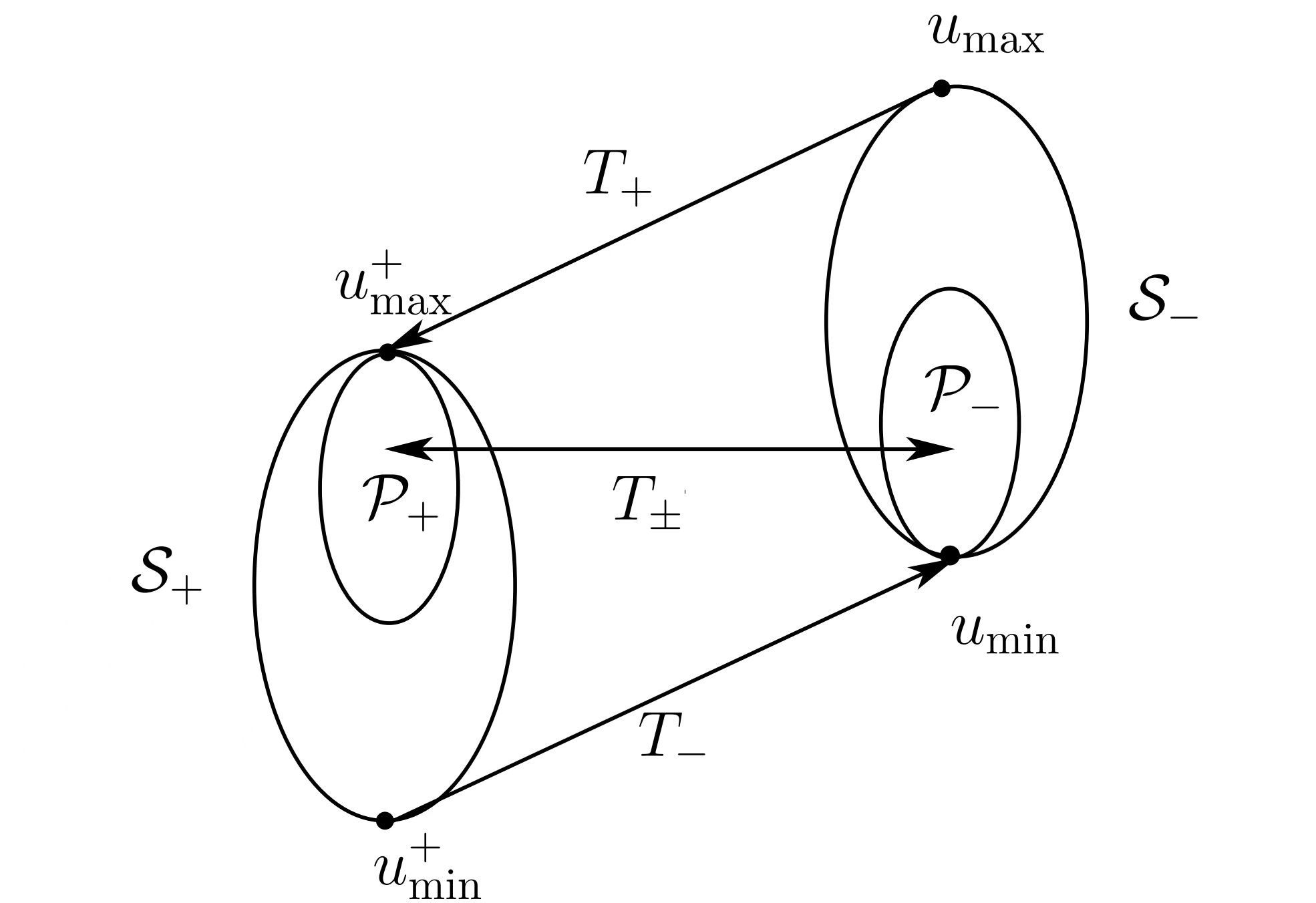
umin+umin=limt+Ttumin+,limt+Tt+umax=umax+umax.u^{+}_{\min}\leq u_{\min}=\lim_{t\to+\infty}T_{t}^{-}u^{+}_{\min},\quad\lim_{t\to+\infty}T_{t}^{+}u_{\max}=u^{+}_{\max}\leq u_{\max}.
Refer to caption
Figure 1: The structure of the solution set of (E0)

Let 𝒮\mathcal{S}_{-} (resp. 𝒮+\mathcal{S}_{+}) be the set of all backward (resp. forward) weak KAM solutions. Given u±𝒮±u_{\pm}\in\mathcal{S}_{\pm}, if

u=limtTtu+,u+=limtTt+u,u_{-}=\lim_{t\to\infty}T_{t}^{-}u_{+},\quad u_{+}=\lim_{t\to\infty}T_{t}^{+}u_{-},

then uu_{-} (resp. u+u_{+}) is called a conjugated backward (resp. forward) weak KAM solution. See Figure 1 for a rough description of structure of the solution set of (E0) in general cases, where 𝕋±:=limtTt±\mathbb{T}_{\pm}:=\lim_{t\to\infty}T_{t}^{\pm}, and 𝒫\mathcal{P}_{-} (resp. 𝒫+\mathcal{P}_{+}) denotes the set of all conjugated backward (resp. forward) weak KAM solutions. For further statement on conjugated weak KAM solutions, one can refer to [10, Theorem 6.5 and Theorem 7.1].

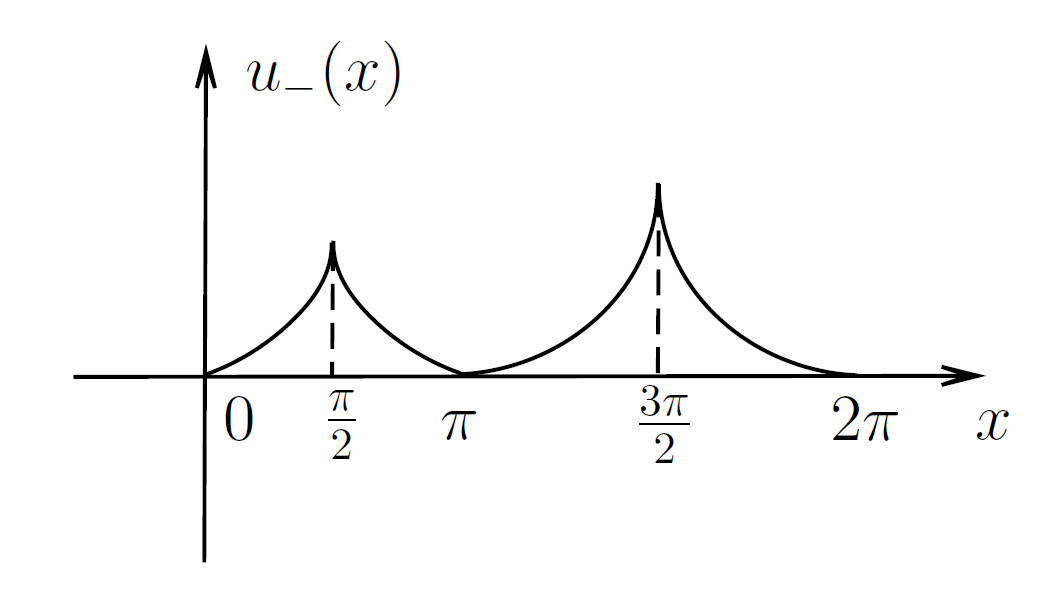
By Proposition 1.2(2), (E0) has at least two solutions if c>c0c>c_{0}. Then a natural question is to figure out what happens if c=c0c=c_{0}. In [11], Jin, Yan and Zhao considered the following example:

Example 1.4.
|u(x)|2+sinxu(x)=c,x𝕊1[0,2π),|u^{\prime}(x)|^{2}+\sin x\cdot u(x)=c,\quad x\in\mathbb{S}^{1}\simeq[0,2\pi), (1.2)

where 𝕊1\mathbb{S}^{1} denotes a flat circle with a fundamental domain [0,2π)[0,2\pi).

It was shown that c0=0c_{0}=0 and there are uncountably many solutions of (1.2) in the critical case. A rough picture of certain solutions is given by Figure 2. See [11, Theorem 3.5] for more details.

Refer to caption
Figure 2: Certain solutions of (1.2) with c=0c=0

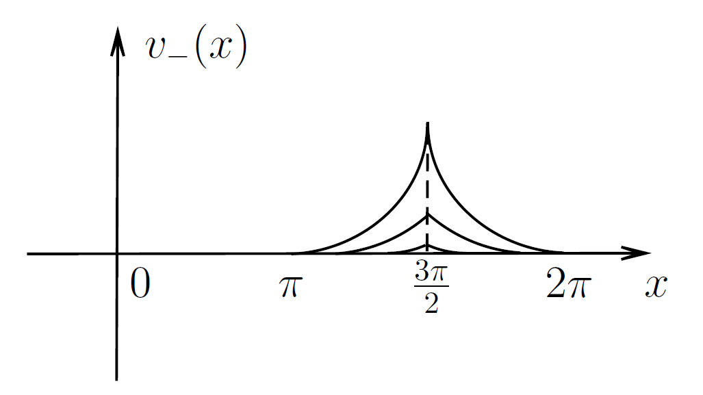
As a complement, we consider

Example 1.5.
12|u(x)|2+sinxu(x)+cos2x1=c,x𝕊1[0,2π).\frac{1}{2}|u^{\prime}(x)|^{2}+\sin x\cdot u(x)+\cos 2x-1=c,\quad x\in\mathbb{S}^{1}\simeq[0,2\pi). (1.3)

We will prove that the critical value is also c0=0c_{0}=0, but (1.3) admits a unique solution in the critical case. A rough picture of the solution is given by Figure 3. See Remark 4.2 below for certain generalization of Example 1.5. Those two examples above show various possibilities about the solution set of (E0) in the critical case.

Refer to caption
Figure 3: The unique solution of (1.3) with c=0c=0

In the second part, we consider the evolutionary equation:

{tu(x,t)+H(x,Du(x,t))+λ(x)u(x,t)=c,(x,t)M×(0,+).u(x,0)=φ(x),xM,\left\{\begin{aligned} &\partial_{t}u(x,t)+H(x,Du(x,t))+\lambda(x)u(x,t)=c,\quad(x,t)\in M\times(0,+\infty).\\ &u(x,0)=\varphi(x),\quad x\in M,\\ \end{aligned}\right. (CP)

where φC(M)\varphi\in C(M). It is well known that the viscosity solution of (CP) is unique (see [10, Corollary 3.2] for instance). By [14, Theorem 1], this solution can be represented by u(x,t):=Ttφ(x)u(x,t):=T_{t}^{-}\varphi(x), where Tt:C(M)C(M)T^{-}_{t}:C(M)\rightarrow C(M) is defined implicitly by

Ttφ(x)=infγ(t)=x{φ(γ(0))+0t[L(γ(τ),γ˙(τ))λ(γ(τ))Tτφ(γ(τ))+c]dτ},T^{-}_{t}\varphi(x)=\inf_{\gamma(t)=x}\left\{\varphi(\gamma(0))+\int_{0}^{t}\bigl{[}L(\gamma(\tau),\dot{\gamma}(\tau))-\lambda(\gamma(\tau))T^{-}_{\tau}\varphi(\gamma(\tau))+c\bigl{]}{d}\tau\right\}, (T-)

where the infimum is taken among absolutely continuous curves γ:[0,t]M\gamma:[0,t]\rightarrow M with γ(t)=x\gamma(t)=x.

In order to obtain equi-Lipschitz continuity of {Ttφ}tδ\{T_{t}^{-}\varphi\}_{t\geq\delta} for a given δ>0\delta>0, we have to strengthen the assumptions on HH from (CON), (CER) to the following:

  • (\star)

    H(x,p)H(x,p) is strictly convex in pp for any xMx\in M, and there is a superlinear function θ:[0,+)[0,+)\theta:[0,+\infty)\to[0,+\infty) such that H(x,p)θ(p)H(x,p)\geq\theta(\|p\|).

Under the assumption (\star), the equi-Lipschitz continuity of {Ttφ}tδ\{T_{t}^{-}\varphi\}_{t\geq\delta} follows from the locally Lipschitz property and boundedness of TtφT_{t}^{-}\varphi on M×(0,+)M\times(0,+\infty). From the weak KAM point of view, that kind of locally Lipschitz property can be verified by a standard procedure once we have the Lipschitz regularity of minimizers of Ttφ(x)T_{t}^{-}\varphi(x) (see [7, Lemma 4.6.3]). However, HH is only supposed to be continuous in our setting. Then one can not use the method of characteristics to improve regularity of these minimizers. Following [2], we will deal with that issue by using the method of energy estimates. A key ingredient of that method is to establish the Erdmann condition for a non-smooth energy function. More precisely, we obtain the following result, whose proof is given in Appendix A.4.

Proposition 1.6.

Assume (\star) holds. If Ttφ(x)T^{-}_{t}\varphi(x) has a bound independent of tt, then the family {Ttφ}tδ\{T_{t}^{-}\varphi\}_{t\geq\delta} is equi-Lipschitz continuous, where δ\delta is an arbitrarily positive constant.

Let us recall umaxu_{\max} denotes the maximal solution of (E0), and umin+u^{+}_{\min} denotes its minimal froward weak KAM solution. By Remark 1.3, umin+umaxu^{+}_{\min}\leq u_{\max} on MM. Both of them play an important role in characterizing the large time behavior of the solution of (CP). By assuming (\star) holds, we obtain the following two results.

Theorem 2.

Let u(x,t)u(x,t) be the solution of (CP) with cc0c\geq c_{0}. Then

  • (1)

    if the initial data φumax\varphi\geq u_{\max}, then u(x,t)u(x,t) converges to umaxu_{\max} uniformly on MM as t+t\to+\infty;

  • (2)

    if there is a point x0Mx_{0}\in M such that φ(x0)<umin+(x0)\varphi(x_{0})<u^{+}_{\min}(x_{0}), then u(x,t)u(x,t) tends to -\infty uniformly on MM as t+t\to+\infty.

Theorem 3.

Let u(x,t)u(x,t) be the solution of (CP) with c>c0c>c_{0}. If the initial data φ>umin+\varphi>u^{+}_{\min}, then u(x,t)u(x,t) converges to umaxu_{\max} uniformly on MM as t+t\to+\infty.

Remark 1.7.

For φumin+\varphi\geq u^{+}_{\min}, if there exists x0Mx_{0}\in M such that φ(x0)=umin+(x0)\varphi(x_{0})=u^{+}_{\min}(x_{0}), then u(x,t)u(x,t) may not converge to umaxu_{\max}.

  • In Example 1.4 with c=0c=0, for each solution vv of (1.2), it is easy to construct an initial data φ\varphi satisfying φ0umin+\varphi\geq 0\geq u^{+}_{\min} and

    {xM|φ(x)=umin+(x)}\{x\in M\ |\ \varphi(x)=u^{+}_{\min}(x)\}\neq\emptyset

    such that u(x,t)u(x,t) converges to vv uniformly on MM. In fact, one can take φ=v\varphi=v for instance.

  • For Example 1.4 with c=1c=1, by [11, Theorem 3.14], umin=sinxumaxu_{\min}=\sin x\neq u_{\max} and

    {xM|umin(x)=umin+(x)}.\{x\in M\ |\ u_{\min}(x)=u^{+}_{\min}(x)\}\neq\emptyset.

    Then one can take φ=sinx\varphi=\sin x such that u(x,t)u(x,t) converges to uminu_{\min} uniformly on MM.

The rest of this paper is organized as follows. Section 2 gives some preliminaries on Tt±T_{t}^{\pm}, weak KAM solutions and Aubry sets. In Section 3, a priori estimates on subsolutions of (E0) are established. The proof of Theorem 1 and a detailed analysis of Example 1.5 are given in Section 4. Theorem 2 and Theorem 3 are proved in Section 5 For the sake of completeness, some auxiliary results are proved in Appendix A.

2 Preliminaries

In this part, we collect some facts on Tt±T_{t}^{\pm}, weak KAM solutions and Aubry sets. These facts hold under more general assumptions on the dependence of uu. Consider the evolutionary equation:

{tu(x,t)+H(x,u(x,t),Du(x,t))=0,(x,t)M×(0,+).u(x,0)=φ(x),xM.\left\{\begin{aligned} &\partial_{t}u(x,t)+H(x,u(x,t),Du(x,t))=0,\quad(x,t)\in M\times(0,+\infty).\\ &u(x,0)=\varphi(x),\quad x\in M.\\ \end{aligned}\right. (A0)

and the stationary equation:

H(x,u(x),Du(x))=0H(x,u(x),Du(x))=0 (B0)

We denote by (x,u,p)(x,u,p) a point in TM×T^{*}M\times\mathbb{R}, where (x,p)TM(x,p)\in T^{*}M and uu\in\mathbb{R}. Let H:TM×H:T^{*}M\times\mathbb{R}\rightarrow\mathbb{R} be a continuous Hamiltonian satisfying

  • (CON):

    H(x,u,p)H(x,u,p) is convex in pp, for any (x,u)M×(x,u)\in M\times\mathbb{R};

  • (CER):

    H(x,u,p)H(x,u,p) is coercive in pp, i.e. limpx+(infxMH(x,0,p))=+\lim_{\|p\|_{x}\rightarrow+\infty}(\inf_{x\in M}H(x,0,p))=+\infty;

  • (LIP):

    H(x,u,p)H(x,u,p) is Lipschitz in uu, uniformly with respect to (x,p)(x,p), i.e., there exists Θ>0\Theta>0 such that |H(x,u,p)H(x,v,p)|Θ|uv||H(x,u,p)-H(x,v,p)|\leq\Theta|u-v|, for all (x,p)TM(x,p)\in\ T^{*}M and all u,vu,v\in\mathbb{R}.

Correspondingly, one has the Lagrangian associated to HH:

L(x,u,x˙):=suppTxM{x˙,pH(x,u,p)}.L(x,u,\dot{x}):=\sup_{p\in T^{*}_{x}M}\{\langle\dot{x},p\rangle-H(x,u,p)\}.

Due to the absence of superlinearity of HH, the corresponding Lagrangian LL may take the value ++\infty. Define

dom(L):={(x,x˙,u)TM×|L(x,u,x˙)<+}.\text{dom}(L):=\{(x,\dot{x},u)\in TM\times\mathbb{R}\ |\ L(x,u,\dot{x})<+\infty\}.

Then L(x,u,x˙)L(x,u,\dot{x}) satisfies the following properties:

  • (LSC):

    L(x,u,x˙)L(x,u,\dot{x}) is lower semicontinuous, and continuous on the interior of dom(L)×\textrm{dom}(L)\times\mathbb{R};

  • (CON):

    L(x,u,x˙)L(x,u,\dot{x}) is convex in x˙\dot{x}, for any (x,u)M×(x,u)\in M\times\mathbb{R};

  • (LIP):

    L(x,u,x˙)L(x,u,\dot{x}) is Lipschitz in uu, uniformly with respect to (x,x˙)(x,\dot{x}), i.e., there exists Θ>0\Theta>0 such that |L(x,u,x˙)L(x,v,x˙)|Θ|uv||L(x,u,\dot{x})-L(x,v,\dot{x})|\leq\Theta|u-v|, for all (x,x˙)dom(L)(x,\dot{x})\in\ \textrm{dom}(L) and all u,vu,v\in\mathbb{R}.

Proposition 2.1.

[14, Theorem 1] Both backward Lax-Oleinik semigroup

Ttφ(x)=infγ(t)=x{φ(γ(0))+0tL(γ(τ),Tτφ(γ(τ)),γ˙(τ))dτ}T^{-}_{t}\varphi(x)=\inf_{\gamma(t)=x}\left\{\varphi(\gamma(0))+\int_{0}^{t}L(\gamma(\tau),T^{-}_{\tau}\varphi(\gamma(\tau)),\dot{\gamma}(\tau))\textrm{d}\tau\right\} (2.1)

and forward Lax-Oleinik semigroup

Tt+φ(x)=supγ(0)=x{φ(γ(t))0tL(γ(τ),Ttτ+φ(γ(τ)),γ˙(τ))𝑑τ}.T^{+}_{t}\varphi(x)=\sup_{\gamma(0)=x}\left\{\varphi(\gamma(t))-\int_{0}^{t}L(\gamma(\tau),T^{+}_{t-\tau}\varphi(\gamma(\tau)),\dot{\gamma}(\tau))d\tau\right\}. (2.2)

are well-defined for φC(M)\varphi\in C(M). The infimum (resp. supremum) is taken among absolutely continuous curves γ:[0,t]M\gamma:[0,t]\rightarrow M with γ(t)=x\gamma(t)=x (resp. γ(0)=x\gamma(0)=x). If φ\varphi is continuous, then u(x,t):=Ttφ(x)u(x,t):=T^{-}_{t}\varphi(x) represents the unique continuous viscosity solution of (A0). If φ\varphi is Lipschitz continuous, then u(x,t):=Ttφ(x)u(x,t):=T^{-}_{t}\varphi(x) is also Lipschitz continuous on M×[0,+)M\times[0,+\infty).

Proposition 2.2.

[14, Proposition 3.1] The Lax-Oleinik semigroups have the following properties

  • (1)

    For φ1\varphi_{1} and φ2C(M)\varphi_{2}\in C(M), if φ1(x)<φ2(x)\varphi_{1}(x)<\varphi_{2}(x) for all xMx\in M, we have Ttφ1(x)<Ttφ2(x)T^{-}_{t}\varphi_{1}(x)<T^{-}_{t}\varphi_{2}(x) and Tt+φ1(x)<Tt+φ2(x)T^{+}_{t}\varphi_{1}(x)<T^{+}_{t}\varphi_{2}(x) for all (x,t)M×(0,+)(x,t)\in M\times(0,+\infty).

  • (2)

    Given any φ\varphi and ψC(M)\psi\in C(M), we have TtφTtψeΘtφψ\|T^{-}_{t}\varphi-T^{-}_{t}\psi\|_{\infty}\leq e^{\Theta t}\|\varphi-\psi\|_{\infty} and Tt+φTt+ψeΘtφψ\|T^{+}_{t}\varphi-T^{+}_{t}\psi\|_{\infty}\leq e^{\Theta t}\|\varphi-\psi\|_{\infty} for all t>0t>0.

Following Fathi [7], one can extend the definitions of backward and forward weak KAM solutions of equation (B0) by using absolutely continuous calibrated curves instead of C1C^{1} curves.

Definition 2.3.

A function uC(M)u_{-}\in C(M) is called a backward weak KAM solution of (B0) if

  • (1)

    For each absolutely continuous curve γ:[t,t]M\gamma:[t^{\prime},t]\rightarrow M, we have

    u(γ(t))u(γ(t))ttL(γ(s),u(γ(s)),γ˙(s))𝑑s.u_{-}(\gamma(t))-u_{-}(\gamma(t^{\prime}))\leq\int_{t^{\prime}}^{t}L(\gamma(s),u_{-}(\gamma(s)),\dot{\gamma}(s))ds.

    The above condition reads that uu_{-} is dominated by LL and denoted by uLu_{-}\prec L.

  • (2)

    For each xMx\in M, there exists an absolutely continuous curve γ:(,0]M\gamma_{-}:(-\infty,0]\rightarrow M with γ(0)=x\gamma_{-}(0)=x such that

    u(x)u(γ(t))=t0L(γ(s),u(γ(s)),γ˙(s))𝑑s,t<0.u_{-}(x)-u_{-}(\gamma_{-}(t))=\int_{t}^{0}L(\gamma_{-}(s),u_{-}(\gamma_{-}(s)),\dot{\gamma}_{-}(s))ds,\quad\forall t<0.

    The curves satisfying the above equality are called (u,L,0)(u_{-},L,0)-calibrated curves.

A forward weak KAM solution of (B0) can be defined in a similar manner. Similar to [19, Proposition 2.8], one has

Proposition 2.4.

Let φC(M)\varphi\in C(M). Then

Tt+(φ)=T¯tφ,Tt(φ)=T¯t+φ,t0.\displaystyle-T^{+}_{t}(-\varphi)=\bar{T}^{-}_{t}\varphi,\quad-T^{-}_{t}(-\varphi)=\bar{T}^{+}_{t}\varphi,\quad\forall t\geq 0. (2.3)

where T¯t±\bar{T}_{t}^{\pm} denote the Lax-Oleinik semigroups associated to L(x,u,x˙)L(x,-u,-\dot{x}).

The following two results are well known for Hamilton-Jacobi equations independent of uu. They are also true in contact cases. We will prove them in Appendixes A.1 and A.2. Proposition 2.5 provides some equivalent characterizations of Lipschitz subsolutions. Proposition 2.6 shows that Tt+T^{+}_{t} is a ‘weak inverse’ of TtT^{-}_{t}.

Proposition 2.5.

Let φLip(M)\varphi\in Lip(M). The following conditions are equivalent:

  • (1)

    φ\varphi is a Lipschitz subsolution of (B0);

  • (2)

    φL\varphi\prec L;

  • (3)

    for each t0t\geq 0,

    TtφφTt+φ.T_{t}^{-}\varphi\geq\varphi\geq T_{t}^{+}\varphi.
Proposition 2.6.

For each φC(M)\varphi\in C(M), we have Tt+TtφφTtTt+φT^{+}_{t}\circ T^{-}_{t}\varphi\leq\varphi\leq T^{-}_{t}\circ T^{+}_{t}\varphi for all t0t\geq 0.

The following three results come from [14], which give some connections among the fixed points of Tt±T_{t}^{\pm}, the lower (resp. upper) half limit, backward (resp. forward) weak KAM solutions and Aubry sets.

Proposition 2.7.

[14, Proposition D.4] Let uC(M)u_{-}\in C(M). The following statements are equivalent:

  • (1)

    uu_{-} is a fixed point of TtT^{-}_{t};

  • (2)

    uu_{-} is a backward weak KAM solution of (B0);

  • (3)

    uu_{-} is a viscosity solution of (B0).

Similarly, let v+C(M)v_{+}\in C(M). The following statements are equivalent:

  • (1’)

    v+v_{+} is a fixed point of Tt+T^{+}_{t};

  • (2’)

    v+v_{+} is a forward weak KAM solution of (B0);

  • (3)’

    v+-v_{+} is a viscosity solution of H(x,u(x),Du(x))=0H(x,-u(x),-Du(x))=0.

Proposition 2.8.

[14, Theorem 3 and Remark 3.5] Let φC(M)\varphi\in C(M).

  • (1)

    If Ttφ(x)T^{-}_{t}\varphi(x) has a bound independent of tt, then the lower half limit

    φˇ(x)=limr0+inf{Ttφ(y):d(x,y)<r,t>1/r}\check{\varphi}(x)=\lim_{r\rightarrow 0+}\inf\{T^{-}_{t}\varphi(y):\ d(x,y)<r,\ t>1/r\}

    is a Lipschitz solution of (B0).

  • (2)

    If Tt+φ(x)T^{+}_{t}\varphi(x) has a bound independent of tt, then the upper half limit

    φ^(x)=limr0+sup{Tt+φ(y):d(x,y)<r,t>1/r},\hat{\varphi}(x)=\lim_{r\rightarrow 0+}\sup\{T^{+}_{t}\varphi(y):\ d(x,y)<r,\ t>1/r\},

    is a Lipschitz forward weak KAM solution of (B0).

  • (3)

    Let uu_{-} be a solution of (B0). Then Tt+uuT_{t}^{+}u_{-}\leq u_{-}. The limit u+:=limt+Tt+uu_{+}:=\lim_{t\rightarrow+\infty}T_{t}^{+}u_{-} exists, and u+u_{+} is a forward weak KAM solution of (B0).

  • (4)

    Let v+v_{+} be a forward weak KAM solution of (B0). Then Ttv+v+T_{t}^{-}v_{+}\geq v_{+}. The limit v:=limt+Ttv+v_{-}:=\lim_{t\rightarrow+\infty}T_{t}^{-}v_{+} exists, and vv_{-} is a solution of (B0).

Proposition 2.9.

[14, Theorem 3] Let uu_{-} (resp. u+u_{+}) be a solution (resp. forward weak KAM solution) of (B0). We define the projected Aubry set with respect to uu_{-} by

u:={xM:u(x)=limt+Tt+u(x)}.\mathcal{I}_{u_{-}}:=\{x\in M:\ u_{-}(x)=\lim_{t\rightarrow+\infty}T^{+}_{t}u_{-}(x)\}.

Correspondingly, we define the projected Aubry set with respect to u+u_{+} by

u+:={xM:u+(x)=limt+Ttu+(x)}.\mathcal{I}_{u_{+}}:=\{x\in M:\ u_{+}(x)=\lim_{t\rightarrow+\infty}T^{-}_{t}u_{+}(x)\}.

Both u\mathcal{I}_{u_{-}} and u+\mathcal{I}_{u_{+}} are nonempty. In particular, if u+(x)=limt+Tt+u(x)u_{+}(x)=\lim_{t\rightarrow+\infty}T^{+}_{t}u_{-}(x) and u(x)=limt+Ttu+(x)u_{-}(x)=\lim_{t\rightarrow+\infty}T^{-}_{t}u_{+}(x), then

u=u+,\mathcal{I}_{u_{-}}=\mathcal{I}_{u_{+}},

which is also denoted by (u,u+)\mathcal{I}_{(u_{-},u_{+})}, following the notation introduced by Fathi [7].

3 Some estimates on subsolutions

In this section, we assume the existence of subsolutions of (E0) and prove some a priori estimates on subsolutions. The existence of subsolutions will be verified for cc0c\geq c_{0} in Proposition A.6 below.

Let L(x,x˙)L(x,\dot{x}) be the Legendre transformation of H(x,p)H(x,p). Let Tt±T_{t}^{\pm} be the Lax-Oleinik semigroups associated to

L(x,x˙)λ(x)u(x)+c.L(x,\dot{x})-\lambda(x)u(x)+c.

Similar to [9, Proposition 2.1], one can prove the local boundedness of L(x,x˙)L(x,\dot{x}) in a neighborhood of the zero section of TMTM.

Lemma 3.1.

Let H(x,p)H(x,p) satisfy (C)(CON)(CER), there exist constants δ>0\delta>0 and CL>0C_{L}>0 such that the Lagrangian L(x,x˙)L(x,\dot{x}) associated to H(x,p)H(x,p) satisfies

L(x,ξ)CL,(x,ξ)M×B¯(0,δ).L(x,\xi)\leq C_{L},\quad\forall(x,\xi)\in M\times\bar{B}(0,\delta). (3.1)

Throughout this paper, we define

μ:=diam(M)/δ,\mu:=\textrm{diam}(M)/\delta, (3.2)

where diam(M)\textrm{diam}(M) denotes the diameter of MM.

Lemma 3.2.

Let φC(M)\varphi\in C(M).

  • (1)

    TtφT^{-}_{t}\varphi has an upper bound independent of tt;

  • (2)

    Tt+φT^{+}_{t}\varphi has a lower bound independent of tt.

Proof.

Take x1Mx_{1}\in M with λ(x1)>0\lambda(x_{1})>0. We first show

Ttφ(x1)max{φ(x1),L(x1,0)+cλ(x1)},t0.T^{-}_{t}\varphi(x_{1})\leq\max\bigg{\{}\varphi(x_{1}),\frac{L(x_{1},0)+c}{\lambda(x_{1})}\bigg{\}},\quad\forall t\geq 0.

Otherwise, there is t>0t>0 such that

Ttφ(x1)>max{φ(x1),L(x1,0)+cλ(x1)}L(x1,0)+cλ(x1).T^{-}_{t}\varphi(x_{1})>\max\bigg{\{}\varphi(x_{1}),\frac{L(x_{1},0)+c}{\lambda(x_{1})}\bigg{\}}\geq\frac{L(x_{1},0)+c}{\lambda(x_{1})}.

There are two cases:

(i) For all s[0,t]s\in[0,t], we have

Tsφ(x1)>L(x1,0)+cλ(x1).T^{-}_{s}\varphi(x_{1})>\frac{L(x_{1},0)+c}{\lambda(x_{1})}.

Take the constant curve γx1\gamma\equiv x_{1}, we have

Ttφ(x1)φ(x1)+0t[L(x1,0)+cλ(x1)Tsφ(x1)]𝑑s<φ(x1),T^{-}_{t}\varphi(x_{1})\leq\varphi(x_{1})+\int_{0}^{t}\bigg{[}L(x_{1},0)+c-\lambda(x_{1})T^{-}_{s}\varphi(x_{1})\bigg{]}ds<\varphi(x_{1}),

which also leads to a contradiction.

(ii) There is t00t_{0}\geq 0 such that

Tt0φ(x1)=L(x1,0)+cλ(x1),T^{-}_{t_{0}}\varphi(x_{1})=\frac{L(x_{1},0)+c}{\lambda(x_{1})},

and

Tsφ(x1)>L(x1,0)+cλ(x1),s(t0,t].T^{-}_{s}\varphi(x_{1})>\frac{L(x_{1},0)+c}{\lambda(x_{1})},\quad\forall s\in(t_{0},t].

Take the constant curve γx1\gamma\equiv x_{1}, we have

Ttφ(x1)Tt0φ(x1)+0t[L(x1,0)+cλ(x1)Tsφ(x1)]𝑑s<L(x1,0)+cλ(x1),T^{-}_{t}\varphi(x_{1})\leq T^{-}_{t_{0}}\varphi(x_{1})+\int_{0}^{t}\bigg{[}L(x_{1},0)+c-\lambda(x_{1})T^{-}_{s}\varphi(x_{1})\bigg{]}ds<\frac{L(x_{1},0)+c}{\lambda(x_{1})},

which leads to a contradiction.

We then prove that for all xMx\in M and all t>0t>0, Ttφ(x)T_{t}^{-}\varphi(x) is bounded from above. It suffices to prove that for all xMx\in M and t>0t>0, Tt+μφ(x)T_{t+\mu}^{-}\varphi(x) is bounded from above, where μ\mu is given by (3.2). Let α:[0,μ]M\alpha:[0,\mu]\rightarrow M be a geodesic connecting x1x_{1} and xx with constant speed, then α˙δ\|\dot{\alpha}\|\leq\delta. Let

K0:=max{φ(x1),L(x1,0)+cλ(x1)}.K_{0}:=\max\bigg{\{}\varphi(x_{1}),\frac{L(x_{1},0)+c}{\lambda(x_{1})}\bigg{\}}.

Given xx1x\neq x_{1}. We assume Tt+μφ(x)>K0T^{-}_{t+\mu}\varphi(x)>K_{0}. Otherwise the proof is completed. Since Ttφ(x1)K0T^{-}_{t}\varphi(x_{1})\leq K_{0}, there exists σ[0,μ)\sigma\in[0,\mu) such that Tt+σφ(α(σ))=K0T^{-}_{{t}+\sigma}\varphi(\alpha(\sigma))=K_{0} and Tt+sφ(α(s))>K0T^{-}_{{t}+s}\varphi(\alpha(s))>K_{0} for all s(σ,μ]s\in(\sigma,\mu]. By definition

Tt+sφ(α(s))\displaystyle T^{-}_{{t}+s}\varphi(\alpha(s)) Tt+σφ(α(σ))+σs[L(α(τ),α˙(τ))λ(α(τ))Tt+τφ(α(τ))+c]𝑑τ\displaystyle\leq T^{-}_{{t}+\sigma}\varphi(\alpha(\sigma))+\int_{\sigma}^{s}\bigg{[}L(\alpha(\tau),\dot{\alpha}(\tau))-\lambda(\alpha(\tau))\cdot T^{-}_{{t}+\tau}\varphi(\alpha(\tau))+c\bigg{]}d\tau
=K0+σs[L(α(τ),α˙(τ))λ(α(τ))Tt+τφ(α(τ))+c]𝑑τ,\displaystyle=K_{0}+\int_{\sigma}^{s}\bigg{[}L(\alpha(\tau),\dot{\alpha}(\tau))-\lambda(\alpha(\tau))\cdot T^{-}_{{t}+\tau}\varphi(\alpha(\tau))+c\bigg{]}d\tau,

which implies

Tt+sφ(α(s))K0σs[L(α(τ),α˙(τ))λ(α(τ))Tt+τφ(α(τ))+c]𝑑τ\displaystyle T^{-}_{{t}+s}\varphi(\alpha(s))-K_{0}\leq\int_{\sigma}^{s}\bigg{[}L(\alpha(\tau),\dot{\alpha}(\tau))-\lambda(\alpha(\tau))\cdot T^{-}_{{t}+\tau}\varphi(\alpha(\tau))+c\bigg{]}d\tau
σs[L(α(τ),α˙(τ))λ(α(τ))K0+c]𝑑τ+λ0σs[Tt+τφ(α(τ))K0]𝑑τ\displaystyle\leq\int_{\sigma}^{s}\bigg{[}L(\alpha(\tau),\dot{\alpha}(\tau))-\lambda(\alpha(\tau))\cdot K_{0}+c\bigg{]}d\tau+\lambda_{0}\int_{\sigma}^{s}\bigg{[}T^{-}_{{t}+\tau}\varphi(\alpha(\tau))-K_{0}\bigg{]}d\tau
L0μ+λ0σs[Tt+τφ(α(τ))K0]𝑑τ,\displaystyle\leq L_{0}\mu+\lambda_{0}\int_{\sigma}^{s}\bigg{[}T^{-}_{{t}+\tau}\varphi(\alpha(\tau))-K_{0}\bigg{]}d\tau,

where λ0\lambda_{0} is given by (1.1) and

L0:=CL+λ0K0+c.L_{0}:=C_{L}+\lambda_{0}K_{0}+c.

where CLC_{L} is given by (3.1). By the Gronwall inequality, we have

Tt+sφ(α(s))K0L0μeλ0(sσ)L0μeλ0μ,s(σ,μ].T^{-}_{{t}+s}\varphi(\alpha(s))-K_{0}\leq L_{0}\mu e^{\lambda_{0}(s-\sigma)}\leq L_{0}\mu e^{\lambda_{0}\mu},\quad\forall s\in(\sigma,\mu].

Take s=μs=\mu we have Tt+μφ(x)K0+L0μeλ0μT^{-}_{{t}+\mu}\varphi(x)\leq K_{0}+L_{0}\mu e^{\lambda_{0}\mu}.

Similar to the argument above, by choosing constant curve γ(τ)x2\gamma(\tau)\equiv x_{2} with τ[0,t]\tau\in[0,t] and replacing Tt+μφT_{t+\mu}^{-}\varphi by Ttμ+φT_{t-\mu}^{+}\varphi, one has

Tt+φ(x)min{φ(x2),L(x2,0)+cλ(x2)}L0μeλ0μ.T_{t}^{+}\varphi(x)\geq\min\bigg{\{}\varphi(x_{2}),\frac{L(x_{2},0)+c}{\lambda(x_{2})}\bigg{\}}-L_{0}\mu e^{\lambda_{0}\mu}. (3.3)

This completes the proof. ∎

Corollary 3.3.

Let u0u_{0} be a Lipschitz subsolution of (E0). Then Ttu0T_{t}^{-}u_{0} (resp. Tt+u0T_{t}^{+}u_{0}) has an upper (resp. lower) bound independent of tt and u0u_{0}.

Proof.

We only prove Ttu0T_{t}^{-}u_{0} has an upper bound independent of tt and u0u_{0}. The case with Tt+u0T_{t}^{+}u_{0} is similar. Let

𝐞0:=min(x,p)TMH(x,p).\mathbf{e}_{0}:=\min_{(x,p)\in T^{*}M}H(x,p). (3.4)

By (CER), 𝐞0\mathbf{e}_{0} is finite. By the definition of the subsolution, H(x1,p)+λ(x1)u0(x1)cH(x_{1},p)+\lambda(x_{1})u_{0}(x_{1})\leqslant c for any pDu0(x1)p\in D^{*}u_{0}(x_{1}), where DD^{*} denotes the reachable gradients. It implies

λ(x1)u0(x1)cmin(x,p)TMH(x,p)=c𝐞0.\lambda(x_{1})u_{0}(x_{1})\leqslant c-\min_{(x,p)\in T^{*}M}H(x,p)=c-\mathbf{e}_{0}.

Hence, for each subsolution u0u_{0}, we have

u0(x1)c𝐞0λ(x1).\displaystyle u_{0}(x_{1})\leq\frac{c-\mathbf{e}_{0}}{\lambda(x_{1})}.

Let

K0:=c𝐞0λ(x1),L0:=CL+λ0K0+c,K_{0}:=\frac{c-\mathbf{e}_{0}}{\lambda(x_{1})},\quad L_{0}:=C_{L}+\lambda_{0}K_{0}+c,

where λ0\lambda_{0} is given by (1.1). Here we note that

L(x1,0)+c=suppTxM(H(x1,p))+cmin(x,p)TMH(x,p)+c=c𝐞0.L(x_{1},0)+c=\sup_{p\in T^{*}_{x}M}(-H(x_{1},p))+c\leq-\min_{(x,p)\in T^{*}M}H(x,p)+c=c-\mathbf{e}_{0}.

By Lemma 3.2, we have

Ttu0(x)K0+L0μeλ0μ.T_{t}^{-}u_{0}(x)\leqslant K_{0}+L_{0}\mu e^{\lambda_{0}\mu}. (3.5)

This completes the proof. ∎

Proposition 3.4.

There exists a constant C>0C>0 such that for any subsolution uu of (E0), there holds

uW1,C.\|u\|_{W^{1,\infty}}\leqslant C.
Proof.

By Proposition 2.5, for each t0t\geq 0,

Tt+uuTtu.T_{t}^{+}u\leq u\leq T_{t}^{-}u.

By Corollary 3.3, there exist C1C_{1}, C2C_{2} independent of uu such that

C2uC1.C_{2}\leq u\leq C_{1}.

For each x,yMx,y\in M, let α:[0,d(x,y)/δ]M\alpha:[0,d(x,y)/\delta]\rightarrow M be a geodesic of length d(x,y)d(x,y) with constant speed α˙=δ\|\dot{\alpha}\|=\delta and connecting xx and yy, where d(x,y)d(x,y) denotes the distance between xx and yy induced by the Riemannian metric gg on MM. Then

L(α(s),α˙(s))CL,s[0,d(x,y)/δ].L(\alpha(s),\dot{\alpha}(s))\leq C_{L},\quad\forall s\in[0,{d(x,y)/\delta}].

By Proposition 2.5,

u(y)u(x)\displaystyle u(y)-u(x) 0d(x,y)/δ[L(α(s),α˙(s))λ(α(s))u(α(s))+c]𝑑s\displaystyle\leq\int_{0}^{d(x,y)/\delta}\bigg{[}L(\alpha(s),\dot{\alpha}(s))-\lambda(\alpha(s))u(\alpha(s))+c\bigg{]}ds
1δ(CL+λ0max{|C1|,|C2|}+c)d(x,y)=:κd(x,y).\displaystyle\leq\frac{1}{\delta}\bigg{(}C_{L}+\lambda_{0}\max\{|C_{1}|,|C_{2}|\}+c\bigg{)}d(x,y)=:\kappa d(x,y).

Note that κ\kappa is independent of the choice of the subsolution uu. We get the equi-Lipschitz continuity of uu by exchanging the role of xx and yy. ∎

Proposition 3.5.

Let u0u_{0} be a Lipschitz subsolution of (E0). Then

u:=limt+Ttu0(x),u+:=limt+Tt+u0(x)u_{-}:=\lim_{t\to+\infty}{T_{t}^{-}}u_{0}(x),\quad u_{+}:=\lim_{t\to+\infty}{T_{t}^{+}}u_{0}(x)

exist, and the limit procedure is uniform in xx. Moreover, uu_{-} is a solution of (E0), and u+u_{+} is a forward weak KAM solution of (E0). In particular, (E0) has a solution uu_{-} for cc0c\geq c_{0}.

Proof.

We only prove that u:=limt+Ttu0(x)u_{-}:=\lim_{t\to+\infty}{T_{t}^{-}}u_{0}(x) exits, and it is a viscosity solution of (E0). The existence of u+u_{+} is similar . By Proposition 2.8

uˇ(x):=limr0+inf{Ttu0(y):d(x,y)<r,t>1/r}\check{u}_{-}(x):=\lim_{r\rightarrow 0+}\inf\{T^{-}_{t}u_{0}(y):\ d(x,y)<r,\ t>1/r\}

is a solution of (E0). By Proposition 2.5(3) and Corollary 3.3, for a given xMx\in M, the limit limt+Ttu0(x)\lim_{t\rightarrow+\infty}T^{-}_{t}u_{0}(x) exists. By definition, we have

uˇ(x)limt+Ttu0(x).\check{u}_{-}(x)\leq\lim_{t\rightarrow+\infty}T^{-}_{t}u_{0}(x).

Using Proposition 2.5(3) again, Ttu0T^{-}_{t}u_{0} is increasing in tt for all t>0t>0, we have

Ttu0(x)\displaystyle T^{-}_{t}u_{0}(x) =limr0+inf{Ttu0(y):d(x,y)<r}\displaystyle=\lim_{r\rightarrow 0+}\inf\{T^{-}_{t}u_{0}(y):\ d(x,y)<r\}
limr0+inf{Tt+su0(y):d(x,y)<r,t+s>1/r}=uˇ(x).\displaystyle\leq\lim_{r\rightarrow 0+}\inf\{{T^{-}_{t+s}}u_{0}(y):\ d(x,y)<r,\ t+s>1/r\}=\check{u}_{-}(x).

Then limt+Ttu0=uˇ\lim_{t\rightarrow+\infty}T^{-}_{t}u_{0}=\check{u}_{-}. Note that uˇ\check{u}_{-} is a solution of (E0). By the Dini theorem, the family {Ttu0}t>0\{T^{-}_{t}u_{0}\}_{t>0} uniformly converges to uˇ\check{u}_{-}. ∎

4 Structure of the solution set of (E0)

Let 𝒮\mathcal{S}_{-} (resp. 𝒮+\mathcal{S}_{+}) be the set of all solutions (resp. forward weak KAM solution) of (E0).

4.1 The maximal solution

We first prove the existence of the maximal solution. Since each solution is a subsolution, by Proposition 3.4, there are C1C_{1} and C2C_{2} such that C2uC1C_{2}\leq u_{-}\leq C_{1} for all u𝒮u_{-}\in\mathcal{S}_{-}. Note that all solutions of (E0) are fixed points of TtT^{-}_{t}. Take a continuous function φ>C1\varphi>C_{1} as the initial data. By Proposition 2.2 (1), TtφT^{-}_{t}\varphi is larger than every solution of (E0). By Lemma 3.2(1), TtφT^{-}_{t}\varphi has an upper bound independent of tt. By Proposition 2.8 (1), the lower half limit

φˇ(x)=limr0+inf{Ttφ(y):d(x,y)<r,t>1/r}\check{\varphi}(x)=\lim_{r\rightarrow 0+}\inf\{T^{-}_{t}\varphi(y):\ d(x,y)<r,\ t>1/r\}

is a Lipschitz continuous viscosity solution of (E0). Since TtφT^{-}_{t}\varphi is larger than every solution of (E0), we have

φˇ(x)\displaystyle\check{\varphi}(x) =limr0+inf{Ttφ(y):d(x,y)<r,t>1/r}\displaystyle=\lim_{r\rightarrow 0+}\inf\{T^{-}_{t}\varphi(y):\ d(x,y)<r,\ t>1/r\}
limr0+inf{v(y):d(x,y)<r}=v(x),\displaystyle\geq\lim_{r\rightarrow 0+}\inf\{v_{-}(y):\ d(x,y)<r\}=v_{-}(x),

for all v𝒮v_{-}\in\mathcal{S}_{-}. Thus, φˇ(x)\check{\varphi}(x) is the maximal solution of (E0).

4.2 The minimal solution

Since each forward weak KAM solution is dominated by L(x,x˙)λ(x)u+cL(x,\dot{x})-\lambda(x)u+c, by Proposition 2.7, it is a subsolution of (E0). By Proposition 3.4, there are C1C_{1} and C2C_{2} such that C2u+C1C_{2}\leq u_{+}\leq C_{1} for all u+𝒮+u_{+}\in\mathcal{S}_{+}. Take a continuous function φ<C2\varphi<C_{2} as the initial data. By Proposition 2.2 (1), Tt+φT^{+}_{t}\varphi is smaller than every forward weak KAM solution of (E0). By Lemma 3.2(2), Tt+φT^{+}_{t}\varphi has a lower bound independent of tt. By Proposition 2.8 (2), the upper half limit

φ^(x)=limr0+sup{Tt+φ(y):d(x,y)<r,t>1/r}\hat{\varphi}(x)=\lim_{r\rightarrow 0+}\sup\{T^{+}_{t}\varphi(y):\ d(x,y)<r,\ t>1/r\}

is a forward weak KAM solution of (E0). Since Tt+φT^{+}_{t}\varphi is smaller than every forward weak KAM solutions of (E0), we have

φ^(x)\displaystyle\hat{\varphi}(x) =limr0+sup{Tt+φ(y):d(x,y)<r,t>1/r}\displaystyle=\lim_{r\rightarrow 0+}\sup\{T^{+}_{t}\varphi(y):\ d(x,y)<r,\ t>1/r\}
limr0+sup{v+(y):d(x,y)<r}=v+(x).\displaystyle\leq\lim_{r\rightarrow 0+}\sup\{v_{+}(y):\ d(x,y)<r\}=v_{+}(x).

for all v+𝒮+v_{+}\in\mathcal{S}_{+}. Thus, φ^(x)\hat{\varphi}(x) is the minimal forward weak KAM solution of (E0). By Proposition 2.8 (4), φ^:=limt+Ttφ^\hat{\varphi}_{\infty}:=\lim_{t\rightarrow+\infty}T^{-}_{t}\hat{\varphi} exists, and it is a solution of (E0).

Lemma 4.1.

φ^\hat{\varphi}_{\infty} is the minimal solution of (E0).

Proof.

Define

𝒫:={u𝒮:u+𝒮+such thatu=limt+Ttu+}.\mathcal{P}_{-}:=\{u_{-}\in\mathcal{S}_{-}:\ \exists u_{+}\in\mathcal{S}_{+}\ \textrm{such\ that}\ u_{-}=\lim_{t\rightarrow+\infty}T^{-}_{t}u_{+}\}.

We first prove that for each v𝒫v_{-}\in\mathcal{P}_{-}, there holds vφ^v_{-}\geq\hat{\varphi}_{\infty}. In fact, by definition of 𝒫\mathcal{P}_{-}, there is u+𝒮+u_{+}\in\mathcal{S}_{+} such that v=limt+Ttu+v_{-}=\lim_{t\rightarrow+\infty}T^{-}_{t}u_{+}. Since φ^\hat{\varphi} is the minimal forward weak KAM solution, we have

u+φ^.u_{+}\geq\hat{\varphi}.

Acting TtT^{-}_{t} on both sides of the inequality above, and letting t+t\rightarrow+\infty, we have vφ^v_{-}\geq\hat{\varphi}_{\infty}.

We then prove that for each v𝒮\𝒫v_{-}\in\mathcal{S}_{-}\backslash\mathcal{P}_{-}, vφ^v_{-}\geq\hat{\varphi}_{\infty} still holds. Let v+:=limt+Tt+vv_{+}:=\lim_{t\rightarrow+\infty}T^{+}_{t}v_{-} and u:=limt+Ttv+u_{-}:=\lim_{t\rightarrow+\infty}T^{-}_{t}v_{+}. Then u𝒫u_{-}\in\mathcal{P}_{-}, which implies uφ^u_{-}\geq\hat{\varphi}_{\infty}. By Proposition 2.8 (3), v+vv_{+}\leq v_{-}. Then we have Ttv+Ttv=vT^{-}_{t}v_{+}\leq T^{-}_{t}v_{-}=v_{-}. Taking t+t\rightarrow+\infty we get uvu_{-}\leq v_{-}. Therefore, vuφ^v_{-}\geq u_{-}\geq\hat{\varphi}_{\infty}. ∎

So far, we complete the proof of Theorem 1.

4.3 On Example (1.5)

The Hamiltonian of (1.3) is formulated as

H(x,u,p)=p22+sinxu+cos2x1.H(x,u,p)=\frac{p^{2}}{2}+\sin x\cdot u+\cos 2x-1. (4.1)

We first show c0=0c_{0}=0. Assume (1.3) admits a smooth subsolution u0u_{0} when c<0c<0, then we have |u0(0)|22c<0|u^{\prime}_{0}(0)|^{2}\leq 2c<0, which is impossible. When c=0c=0, the constant function φ0\varphi\equiv 0 is a subsolution of (1.3). Therefore c0=0c_{0}=0. By Proposition 3.5, there is a solution uu_{-} of (1.3) given by

u:=limt+Ttφ.u_{-}:=\lim_{t\to+\infty}T_{t}^{-}\varphi.

Since TtφφT_{t}^{-}\varphi\geq\varphi, then u0u_{-}\geq 0.

We then divide the proof into the following steps:

  • In Step 1, we discuss the dynamical behavior of the contact Hamiltonian flow ΦtH\Phi^{H}_{t} generated by H(x,u,p)H(x,u,p), which is restricted on a two dimensional energy shell M0M^{0}.

    \centerdot In Step 1.1, we show that the non-wandering set of ΦtH\Phi^{H}_{t} consists of four fixed points;

    \centerdot In Step 1.2, we classify these fixed points by linearization;

    \centerdot In Step 1.3, we show that for each solution vv_{-} of (1.3), the α\alpha-limit set of any (v,L,0)(v_{-},L,0)-calibrated curve γ:(,0]𝕊1\gamma:(-\infty,0]\rightarrow\mathbb{S}^{1} with γ(0)π/2\gamma(0)\neq\pi/2 and 3π/23\pi/2 can only be 0 or π\pi. We only focus on the projected α\alpha-limit set defined on 𝕊1\mathbb{S}^{1}. For simplicity, we define

    α(γ):={x𝕊1:there exists a sequencetnsuch that|γ(tn)x|0},\alpha(\gamma):=\{{x\in\mathbb{S}^{1}}:\ \textrm{there\ exists\ a\ sequence}\ t_{n}\rightarrow-\infty\ \textrm{such\ that}\ {|\gamma(t_{n})-x|\to 0}\},

    where γ:(,0]𝕊1\gamma:(-\infty,0]\rightarrow\mathbb{S}^{1} is a (v,L,0)(v_{-},L,0)-calibrated curve. Moreover, we check the constant curves γ(t)0,π\gamma(t)\equiv 0,\pi are calibrated curves, which implies v(0)=v(π)=0v_{-}(0)=v_{-}(\pi)=0, v(0)=v(π)=0v^{\prime}_{-}(0)=v^{\prime}_{-}(\pi)=0.

  • In Step 2, we prove the uniqueness of the solution vv_{-} of (1.3).

    \centerdot In Step 2.1, we prove that vv_{-} is unique near 0 and π\pi;

    \centerdot In Step 2.2, we prove that vv_{-} is unique on [π,2π)[\pi,2\pi) by the comparison along calibrated curves via the Gronwall inequality. The uniqueness of vv_{-} on [0,π][0,\pi] is guaranteed by the comparison principle for the Dirichlet problem.

Step 1. The dynamical behavior of the contact Hamiltonian flow.

For each solution vv_{-} of (1.3), let γ:(,0]𝕊1\gamma:(-\infty,0]\rightarrow\mathbb{S}^{1} be a (v,L,0)(v_{-},L,0)-calibrated curve. Similar to the analysis at the beginning of [11, Section 3.2], the derivative v(γ(t))v^{\prime}_{-}(\gamma(t)) exists for each t(,0)t\in(-\infty,0) and the orbit (γ(t),v(γ(t)),v(γ(t)))(\gamma(t),v_{-}(\gamma(t)),v^{\prime}_{-}(\gamma(t))) satisfies the contact Hamilton equations generated by the Hamiltonian H(x,u,p)H(x,u,p) defined in (4.1). Then the proof of the uniqueness of the solution of (1.3) is related to the contact Hamiltonian flow ΦtH\Phi^{H}_{t} generated by H(x,u,p)H(x,u,p).

Since c0=0c_{0}=0 and H(γ(t),v(γ(t)),v(γ(t)))=0H(\gamma(t),v_{-}(\gamma(t)),v^{\prime}_{-}(\gamma(t)))=0 for t(,0)t\in(-\infty,0), we discuss the flow on the two dimensional energy shell

M0:={(x,u,p)T𝕊1×:H(x,u,p)=0}.M^{0}:=\{(x,u,p)\in T^{*}\mathbb{S}^{1}\times\mathbb{R}:\ H(x,u,p)=0\}.

Note that along the contact Hamiltonian flow, we have dH/dt=HH/udH/dt=-H\partial H/\partial u, which equals to zero on the set M0M^{0}. Thus, M0M^{0} is an invariant set under the action of ΦtH\Phi^{H}_{t}. Since we are interested in the orbit (γ(t),v(γ(t)),v(γ(t)))(\gamma(t),v_{-}(\gamma(t)),v^{\prime}_{-}(\gamma(t))), we then consider the flow ΦtH\Phi^{H}_{t} restrict on M0M^{0}. The contact Hamilton equations then reduce to

{x˙=p,p˙=(cosxu2sin2x)sinxp,u˙=p2.\left\{\begin{aligned} &\dot{x}=p,\\ &\dot{p}=-(\cos x\cdot u-2\sin 2x)-\sin x\cdot p,\\ &\dot{u}=p^{2}.\\ \end{aligned}\right. (4.2)

Step 1.1. The non-wandering set. We first consider the non-wandering set Ω\Omega of ΦtH|M0\Phi^{H}_{t}|_{M^{0}}. Suppose there is an orbit (x(t),u(t),p(t))(x(t),u(t),p(t)) belongs to Ω\Omega. Since u˙=p20\dot{u}=p^{2}\geq 0, u(t)u(t) equals to a constant cuc_{u} and p(t)0p(t)\equiv 0. By x˙(t)=p(t)=0\dot{x}(t)=p(t)=0, x(t)x(t) also equals to a constant cxc_{x}. By H(x,u,p)=0H(x,u,p)=0 and p=0p=0, we have

sinxu+cos2x1=0.\sin x\cdot u+\cos 2x-1=0.

By p=0p=0 and p˙=0\dot{p}=0 we have

cosxu2sin2x=0.\cos x\cdot u-2\sin 2x=0.

A direct calculation shows that the only non-wandering points are

P1=(0,0,0),P2=(π,0,0),P3=(π2,2,0),P4=(3π2,2,0).P_{1}=(0,0,0),\quad P_{2}=(\pi,0,0),\quad P_{3}=(\frac{\pi}{2},2,0),\quad P_{4}=(\frac{3\pi}{2},-2,0).

Step 1.2. The classification of fixed points. We then consider the dynamical behavior of ΦtH|M0\Phi^{H}_{t}|_{M^{0}} near the fixed points. After a translation, we put the fixed points to be the origin. Near the points P1P_{1} and P2P_{2}, the linearised equation of (4.2) is

x˙=p,p˙=4x,u˙=0.\dot{x}=p,\quad\dot{p}=4x,\quad\dot{u}=0.

Thus, P1P_{1} and P2P_{2} are hyperbolic fixed points for the dynamical system ΦtH|M0\Phi^{H}_{t}|_{M^{0}}. Near the points P3P_{3} and P4P_{4}, the linearised equations of (4.2) are

x˙=p,p˙=2xp,u˙=0\dot{x}=p,\quad\dot{p}=-2x-p,\quad\dot{u}=0

and

x˙=p,p˙=2x+p,u˙=0\dot{x}=p,\quad\dot{p}=-2x+p,\quad\dot{u}=0

respectively. Thus, P3P_{3} is a stable focus, and P4P_{4} is an unstable focus.

Step 1.3. The α\alpha-limit set of calibrated curves. The α\alpha-limit set of a (v,L,0)(v_{-},L,0)-calibrated curve γ\gamma is contained in the projection of Ω\Omega. If γ\gamma itself is not a fixed point, and the α\alpha-limit of γ\gamma is a focus, then there are two constants t1<t2<0t_{1}<t_{2}<0 with γ(t1)=γ(t2)\gamma(t_{1})=\gamma(t_{2}) such that v(γ(t1))v(γ(t2))v^{\prime}_{-}(\gamma(t_{1}))\neq v^{\prime}_{-}(\gamma(t_{2})), which is impossible. In other words, the obits near a focus can not form a 1-graph. Thus, the α\alpha-limit of γ:(,0]𝕊1\gamma:(-\infty,0]\rightarrow\mathbb{S}^{1} with γ(0)π/2,3π/2\gamma(0)\neq\pi/2,3\pi/2 can only be either 0 or π\pi. For constant curve γ:(,0]𝕊1\gamma:(-\infty,0]\rightarrow\mathbb{S}^{1} with γ(t)x0\gamma(t)\equiv x_{0} and x0x_{0} equals to either 0 or π\pi, we have

v(x0)v(x0)=0=0tL(x0,v(x0),0)𝑑s,v_{-}(x_{0})-v_{-}(x_{0})=0=\int_{0}^{t}L(x_{0},v_{-}(x_{0}),0)ds,

where

L(x,u,x˙)=x˙22sinxucos2x+1L(x,u,\dot{x})=\frac{\dot{x}^{2}}{2}-\sin x\cdot u-\cos 2x+1

is the Lagrangian corresponding to H(x,u,p)H(x,u,p). Then the constant curve γ\gamma is a (v,L,0)(v_{-},L,0)-calibrated curve. We then have

limtv(γ(t))=v(0)=v(π)=cu=0,\lim_{t\rightarrow-\infty}v_{-}(\gamma(t))=v_{-}(0)=v_{-}(\pi)=c_{u}=0,

and

limtv(γ(t))=v(0)=v(π)=0.\lim_{t\rightarrow-\infty}v^{\prime}_{-}(\gamma(t))=v^{\prime}_{-}(0)=v^{\prime}_{-}(\pi)=0.

Step 2. The uniqueness of the solution vv_{-} of (1.3).

Step 2.1. For x𝕊1\{π/2,3π/2}x\in\mathbb{S}^{1}\backslash\{\pi/2,3\pi/2\}, let γ:(,0]𝕊1\gamma:(-\infty,0]\rightarrow\mathbb{S}^{1} with γ(0)=x\gamma(0)=x be a (v,L,0)(v_{-},L,0)-calibrated curve. We claim that there is a constant δ>0\delta>0 such that for x[0,δ]x\in[0,\delta], the α\alpha-limit of the calibrated curve γ\gamma is 0. If not, the α\alpha-limit of γ\gamma is π\pi for all x(0,π]x\in(0,\pi]. Then vv_{-} is decreasing on (0,π](0,\pi], since vv_{-} is increasing along γ\gamma by the last equality of (4.2). By Step 1.3, v(0)=v(π)=0v_{-}(0)=v_{-}(\pi)=0, we get v0v_{-}\equiv 0 on [0,π][0,\pi], which is impossible. By similar arguments, we conclude that there is a constant δ>0\delta>0 such that the α\alpha-limit of γ\gamma is 0 for x[0,δ][2πδ,2π)x\in[0,\delta]\cup[2\pi-\delta,2\pi), and the α\alpha-limit of γ\gamma is π\pi for x[πδ,π+δ]x\in[\pi-\delta,\pi+\delta]. Shrink δ\delta if necessary, the 1-graph (x,v(x),v(x))(x,v_{-}(x),v^{\prime}_{-}(x)) coincides with the local unstable manifold of P1P_{1} (resp. P2P_{2}) corresponding to the restricted flow ΦtH|M0\Phi^{H}_{t}|_{M^{0}} when x[0,δ][2πδ,2π)x\in[0,\delta]\cup[2\pi-\delta,2\pi) (resp. x[πδ,π+δ]x\in[\pi-\delta,\pi+\delta]). Therefore, the solution vv_{-} is unique on [0,δ][2πδ,2π)[πδ,π+δ][0,\delta]\cup[2\pi-\delta,2\pi)\cup[\pi-\delta,\pi+\delta].

Step 2.2. Since sinxsinδ>0\sin x\geq\sin\delta>0 for x[δ,πδ]x\in[\delta,\pi-\delta], by the uniqueness of the solution of the Dirichlet problem (cf. [4, Theorem 3.3]), vv_{-} is unique on [0,π][0,\pi]. It remains to consider the uniqueness of vv_{-} for x[π,2π)x\in[\pi,2\pi). Assume that there are two solutions uu_{-} and vv_{-} satisfying u(x)>v(x)u_{-}(x)>v_{-}(x) at some point x(π+δ,3π/2)x\in(\pi+\delta,3\pi/2). Let γ\gamma be a (v,L,0)(v_{-},L,0)-calibrated curve with γ(0)=x\gamma(0)=x. Without any loss of generality, we assume the α\alpha-limit of γ\gamma is π\pi. Take t0<0t_{0}<0 such that γ(t0)=π+δ\gamma(t_{0})=\pi+\delta, and define

G(s):=u(γ(s))v(γ(s)),s[t0,0].G(s):=u_{-}(\gamma(s))-v_{-}(\gamma(s)),\quad s\in[t_{0},0].

Then G(t0)=0G(t_{0})=0 and G(0)>0G(0)>0. By continuity, there is σ0[t0,0)\sigma_{0}\in[t_{0},0) such that G(σ0)=0G(\sigma_{0})=0 and G(σ)>0G(\sigma)>0 for all σ(σ0,0]\sigma\in(\sigma_{0},0]. By definition we have

u(γ(σ))u(γ(σ0))σ0σL(γ(s),u(γ(s)),γ˙(s))𝑑s,u_{-}(\gamma(\sigma))-u_{-}(\gamma(\sigma_{0}))\leq\int_{\sigma_{0}}^{\sigma}L(\gamma(s),u_{-}(\gamma(s)),\dot{\gamma}(s))ds,

and

v(γ(σ))v(γ(σ0))=σ0σL(γ(s),v(γ(s)),γ˙(s))𝑑s,v_{-}(\gamma(\sigma))-v_{-}(\gamma(\sigma_{0}))=\int_{\sigma_{0}}^{\sigma}L(\gamma(s),v_{-}(\gamma(s)),\dot{\gamma}(s))ds,

which implies

G(σ)σ0σG(s)𝑑s.G(\sigma)\leq\int_{\sigma_{0}}^{\sigma}G(s)ds.

By the Gronwall inequality, we have G(σ)0G(\sigma)\equiv 0 for all σ(σ0,0]\sigma\in(\sigma_{0},0], which contradicts u(x)>v(x)u_{-}(x)>v_{-}(x). The case x(3π/2,2πδ)x\in(3\pi/2,2\pi-\delta) is similar. By the continuity of vv_{-} at 3π/23\pi/2, we finally conclude that the solution is unique on [π,2π)[\pi,2\pi).

Remark 4.2.

The method introduced in this section can be generalized to the following case

H(x,Du)+λ(x)u=c,x𝕊1,H(x,Du)+\lambda(x)u=c,\quad x\in\mathbb{S}^{1},

where λ(x)\lambda(x) and H(x,p)H(x,p) are of class C3C^{3} and

  • (i)

    the zero points of λ(x)\lambda(x) are x1x_{1} and x2x_{2}, and λ(x)0\lambda^{\prime}(x)\neq 0 at x1x_{1} and x2x_{2};

  • (ii)

    H(x,p)H(x,p) is strictly convex and superlinear in pp, H(x,p)H(x,p)H(x,p)\equiv H(x,-p),

    maxx𝕊1H(x,0)=0\max_{x\in\mathbb{S}^{1}}H(x,0)=0

    and the maximum is achieved at x1x_{1} and x2x_{2}, and the Hessian matrix of HH is negative definite at (x1,0)(x_{1},0) and (x2,0)T𝕊1(x_{2},0)\in T^{*}\mathbb{S}^{1};

  • (iii)

    for all x𝕊1x\in\mathbb{S}^{1}, let γ:(,0]𝕊1\gamma:(-\infty,0]\to\mathbb{S}^{1} with γ(0)=x\gamma(0)=x be a calibrated curve, then the α\alpha-limit of γ\gamma is either x1x_{1} or x2x_{2}.

By (ii), H(x,p)H(x,0)H(x,p)\geq H(x,0), where the equality holds if and only if p=0p=0. By the argument at the beginning of this section, it is direct to see the critical value c0=0c_{0}=0. Now let c=0c=0. The contact Hamilton equations for ΦtH|M0\Phi^{H}_{t}|_{M^{0}} are

{x˙=Hp(x,p),p˙=Hx(x,p)λ(x)uλ(x)p,u˙=Hp(x,p)p.\left\{\begin{aligned} &\dot{x}=\frac{\partial H}{\partial p}(x,p),\\ &\dot{p}=-\frac{\partial H}{\partial x}(x,p)-\lambda^{\prime}(x)u-\lambda(x)p,\\ &\dot{u}=\frac{\partial H}{\partial p}(x,p)p.\\ \end{aligned}\right. (4.3)

By (ii), u˙0\dot{u}\geq 0 and the equality holds if and only if p=0p=0. By the second equation in (4.3), there is only one non-wandering point of ΦtH|M0\Phi^{H}_{t}|_{M^{0}} over x1x_{1} (resp. x2x_{2})

P1=(x1,0,0)(resp.P2=(x2,0,0))P_{1}=(x_{1},0,0)\quad\textrm{(resp.}\ P_{2}=(x_{2},0,0)\textrm{)}

Note that

L(x,0)=suppT𝕊1H(x,p)=infpT𝕊1H(x,p)=H(x,0).L(x,0)=\sup_{p\in T^{*}\mathbb{S}^{1}}-H(x,p)=-\inf_{p\in T^{*}\mathbb{S}^{1}}H(x,p)=-H(x,0).

Similar to Step 1.3 above, we have v(x1)=v(x2)=0v_{-}(x_{1})=v_{-}(x_{2})=0 for each solution vv_{-}. Near the points P1P_{1} and P2P_{2}, the linearised equation is

x˙=2Hxpx+2Hp2p,p˙=2Hx2x2Hxpp,u˙=0,\dot{x}=\frac{\partial^{2}H}{\partial x\partial p}x+\frac{\partial^{2}H}{\partial p^{2}}p,\quad\dot{p}=-\frac{\partial^{2}H}{\partial x^{2}}x-\frac{\partial^{2}H}{\partial x\partial p}p,\quad\dot{u}=0,

By (ii), P1P_{1} and P2P_{2} are hyperbolic fixed points. By (iii) and u˙0\dot{u}\geq 0, the solution is unique near x1x_{1} and x2x_{2}. The remaining proof is similar to Step 2.2 above, we omit it for brevity.

5 Large time behavior of the solution of (CP)

Let us recall umaxu_{\max} (resp. umin+u_{\min}^{+}) be the maximal solution (resp. minimal forward weak KAM solution) of (E0). These two solutions play an important role in characterizing the large time behavior of the solution of (CP).

5.1 Above the maximal solution

Let φumax\varphi\geq u_{\max}. Then TtφumaxT_{t}^{-}\varphi\geq u_{\max}. Combining with Lemma 3.2(1), Ttφ(x)T^{-}_{t}\varphi(x) has a bound independent of tt. Then the pointwise limit

u¯(x):=lim supt+Ttφ(x)\bar{u}(x):=\limsup_{t\rightarrow+\infty}T^{-}_{t}\varphi(x)

exists.

Assume (\star) holds. By Proposition 1.6, the family {Ttφ(x)}t1\{T^{-}_{t}\varphi(x)\}_{t\geq 1} is equi-Lipschitz in xx. We denote by κ\kappa the Lipschitz constant of Ttφ(x)T^{-}_{t}\varphi(x) in xx. Since

|supstTsφ(x)supstTsφ(y)|supst|Tsφ(x)Tsφ(y)|κd(x,y),|\sup_{s\geq t}T^{-}_{s}\varphi(x)-\sup_{s\geq t}T^{-}_{s}\varphi(y)|\leq\sup_{s\geq t}|T^{-}_{s}\varphi(x)-T^{-}_{s}\varphi(y)|\leq\kappa d(x,y),

the limiting procedure

u¯(x)=limt+supstTsφ(x)\bar{u}(x)=\lim_{t\rightarrow+\infty}\sup_{s\geq t}T^{-}_{s}\varphi(x)

is uniform in xx. Thus, the function u¯(x)\bar{u}(x) is Lipschitz continuous. We assert that u¯\bar{u} is a subsolution. If the assertion is true, by Proposition 3.5, limt+Ttu¯(x)\lim_{t\rightarrow+\infty}T^{-}_{t}\bar{u}(x) exits, and it is a solution. Since TtφumaxT^{-}_{t}\varphi\geq u_{\max}, we have u¯umax\bar{u}\geq u_{\max}. Thus, limt+Ttu¯=umax\lim_{t\rightarrow+\infty}T^{-}_{t}\bar{u}=u_{\max}. Based on Section 4.1, the lower half limit φˇ=umax\check{\varphi}=u_{\max}. By the definition of φˇ\check{\varphi}, we have

lim inft+Ttφ(x)φˇ(x)=umax.\liminf_{t\rightarrow+\infty}T^{-}_{t}\varphi(x)\geq\check{\varphi}(x)=u_{\max}.

On the other hand,

lim supt+Ttφ(x)=u¯(x)limt+Ttu¯(x)=umax(x).\limsup_{t\rightarrow+\infty}T^{-}_{t}\varphi(x)=\bar{u}(x)\leq\lim_{t\rightarrow+\infty}T^{-}_{t}\bar{u}(x)=u_{\max}(x).

It follows that limt+Ttφ=umax\lim_{t\rightarrow+\infty}T^{-}_{t}\varphi=u_{\max} uniformly on MM.

It remains to prove u¯\bar{u} is a subsolution. By Proposition 2.5, we only need to show Ttu¯T^{-}_{t}\bar{u} is increasing in tt.

We claim that for every ε>0\varepsilon>0, there exists a constant s0>0s_{0}>0 independent of xx such that for any ss0s\geq s_{0},

Tsφ(x)u¯(x)+ε.T^{-}_{s}\varphi(x)\leq\bar{u}(x)+\varepsilon.

Fixing xMx\in M, by definition of lim sup\limsup, for every ε>0\varepsilon>0, there is s0(x)>0s_{0}(x)>0 such that for any ss0(x)s\geq s_{0}(x),

Tsφ(x)u¯(x)+ε3.T^{-}_{s}\varphi(x)\leq\bar{u}(x)+\frac{\varepsilon}{3}.

Take r:=ε3κr:=\frac{\varepsilon}{3\kappa}. For ss0(x)s\geq s_{0}(x), we have

Tsφ(y)\displaystyle T^{-}_{s}\varphi(y) Tsφ(x)+κd(x,y)u¯(x)+ε3+κd(x,y)\displaystyle\leq T^{-}_{s}\varphi(x)+\kappa d(x,y)\leq\bar{u}(x)+\frac{\varepsilon}{3}+\kappa d(x,y)
u¯(y)+ε3+2κd(x,y)u¯(y)+ε,yBr(x).\displaystyle\leq\bar{u}(y)+\frac{\varepsilon}{3}+2\kappa d(x,y)\leq\bar{u}(y)+\varepsilon,\quad\forall y\in B_{r}(x).

Since MM is compact, there are finite points xiMx_{i}\in M such that for each yMy\in M, there is a point xix_{i} such that yBr(xi)y\in B_{r}(x_{i}). Let s0:=maxis0(xi)s_{0}:=\max_{i}s_{0}(x_{i}) and the claim is proved.

By Proposition 2.2, for each t>0t>0 we have

Tt(Tsφ(x))Tt(u¯(x)+ε)Ttu¯(x)+εeλ0t,T^{-}_{t}(T^{-}_{s}\varphi(x))\leq T^{-}_{t}(\bar{u}(x)+\varepsilon)\leq T^{-}_{t}\bar{u}(x)+\varepsilon e^{\lambda_{0}t},

where λ0:=λ(x)>0\lambda_{0}:=\|\lambda(x)\|_{\infty}>0. Taking the limit s+s\rightarrow+\infty, we have

u¯(x)=lim sups+Tt(Tsφ(x))Ttu¯(x)+εeλ0t.\bar{u}(x)=\limsup_{s\rightarrow+\infty}T^{-}_{t}(T^{-}_{s}\varphi(x))\leq T^{-}_{t}\bar{u}(x)+\varepsilon e^{\lambda_{0}t}.

Letting ε0+\varepsilon\rightarrow 0+, we get u¯(x)Ttu¯(x)\bar{u}(x)\leq T^{-}_{t}\bar{u}(x), which means Ttu¯(x)T^{-}_{t}\bar{u}(x) is increasing in tt.

5.2 Below the minimal solution

We have proved that for each φumax\varphi\geq u_{\max}, limt+Ttφ=umax\lim_{t\rightarrow+\infty}T^{-}_{t}\varphi=u_{\max} uniformly on MM. Combining with Proposition 2.4 and Proposition 2.7, one has

Lemma 5.1.

Let φC(M)\varphi\in C(M). If φumin+\varphi\leq u^{+}_{\min}, then limt+Tt+φ=umin+\lim_{t\rightarrow+\infty}T^{+}_{t}\varphi=u^{+}_{\min} uniformly on MM.

Lemma 5.2.

Let φC(M)\varphi\in C(M) and there is a point x0Mx_{0}\in M such that φ(x0)<umin+(x0)\varphi(x_{0})<u_{\min}^{+}(x_{0}), then Ttφ(x)T^{-}_{t}\varphi(x) tends to -\infty uniformly on MM as t+t\rightarrow+\infty.

Proof.

We first prove that minxMTtφ(x)\min_{x\in M}T^{-}_{t}\varphi(x) tends to -\infty as t+t\rightarrow+\infty. We argue by contradiction. Assume there is a constant K1K_{1} and a sequence {tn}n\{t_{n}\}_{n\in\mathbb{N}} such that TtnφK1T^{-}_{t_{n}}\varphi\geq K_{1}. By Lemma 3.2, TtnφT^{-}_{t_{n}}\varphi also has a upper bound independent of tt. Thus, the function vn(x):=Ttnφ(x)v_{n}(x):=T^{-}_{t_{n}}\varphi(x) is bounded continuous for each nn. By Proposition 2.6, we have φ(x0)Ttn+vn(x0)\varphi(x_{0})\geq T^{+}_{t_{n}}v_{n}(x_{0}). By Proposition 3.4, all of subsolutions are uniformly bounded. Denote by K2K_{2} their lower bound. Let K:=min{K1,K2}K^{\prime}:=\min\{K_{1},K_{2}\}, then Ttn+vnTtn+KT^{+}_{t_{n}}v_{n}\geq T^{+}_{t_{n}}K^{\prime}. By Lemma 3.2(2), Tt+KT^{+}_{t}K^{\prime} has a lower bound independent of tt. Since KK2K^{\prime}\leq K_{2}, Tt+KT^{+}_{t}K^{\prime} is smaller than every forward weak KAM solution of (E0). By Lemma 5.1, limt+Tt+K\lim_{t\rightarrow+\infty}T^{+}_{t}K^{\prime} exists and it equals to umin+u^{+}_{\min}. We conclude

umin+(x0)lim suptn+Ttn+vn(x0)φ(x0)<umin+(x0),u^{+}_{\min}(x_{0})\leq\limsup_{t_{n}\to+\infty}T^{+}_{t_{n}}v_{n}(x_{0})\leq\varphi(x_{0})<u^{+}_{\min}(x_{0}),

which leads to a contradiction.

We then prove that Ttφ(x)T^{-}_{t}\varphi(x) tends to -\infty uniformly as t+t\rightarrow+\infty. Let W(x)W(x) be the inverse function of xxexx\mapsto xe^{x}. Take 0<ηW(1)/λ00<\eta\leq W(1)/\lambda_{0}. We define K(t):=minxMTtφ(x)K(t):=\min_{x\in M}T^{-}_{t}\varphi(x), which tends to -\infty as t+t\to+\infty. We take an arbitrary xMx\in M. If Tt+ηφ(x)K(t)T^{-}_{t+\eta}\varphi(x)\leq K(t), then the proof is finished. So we assume Tt+ηφ(x)>K(t)T^{-}_{t+\eta}\varphi(x)>K(t). Let xtx_{t} be the minimal point of TtφT^{-}_{t}\varphi. Take a geodesic α:[0,η]M\alpha:[0,\eta]\to M with α(0)=xt\alpha(0)=x_{t}, α(η)=x\alpha(\eta)=x and constant speed α˙diam(M)/η\|\dot{\alpha}\|\leq\textrm{diam}(M)/\eta. By continuity, there is σ[0,η)\sigma\in[0,\eta) such that Tt+σφ(α(σ))=K(t)T^{-}_{t+\sigma}\varphi(\alpha(\sigma))=K(t) and Tt+sφ(α(s))>K(t)T^{-}_{t+s}\varphi(\alpha(s))>K(t) for all s(σ,η]s\in(\sigma,\eta]. Then

Tt+sφ(α(s))Tt+σφ(α(σ))+σs[L(α(τ),α˙(τ))λ(α(τ))Tt+τφ(α(τ))+c]𝑑τ\displaystyle T^{-}_{{t}+s}\varphi(\alpha(s))\leq T^{-}_{t+\sigma}\varphi(\alpha(\sigma))+\int_{\sigma}^{s}\bigg{[}L(\alpha(\tau),\dot{\alpha}(\tau))-\lambda(\alpha(\tau))\cdot T^{-}_{{t}+\tau}\varphi(\alpha(\tau))+c\bigg{]}d\tau
K(t)+σs[L(α(τ),α˙(τ))λ0K(t)+c]𝑑τ+λ0σs[Tt+τφ(α(τ))K(t)]𝑑τ\displaystyle\leq K(t)+\int_{\sigma}^{s}\bigg{[}L(\alpha(\tau),\dot{\alpha}(\tau))-\lambda_{0}K(t)+c\bigg{]}d\tau+\lambda_{0}\int_{\sigma}^{s}\bigg{[}T^{-}_{{t}+\tau}\varphi(\alpha(\tau))-K(t)\bigg{]}d\tau
K(t)+C¯Lηλ0ηK(t)+λ0σs[Tt+τφ(α(τ))K(t)]𝑑τ,\displaystyle\leq K(t)+\bar{C}_{L}\eta-\lambda_{0}\eta K(t)+\lambda_{0}\int_{\sigma}^{s}\bigg{[}T^{-}_{{t}+\tau}\varphi(\alpha(\tau))-K(t)\bigg{]}d\tau,

where

C¯L:=maxxM,x˙diam(M)/η|L(x,x˙)+c|\bar{C}_{L}:=\max_{x\in M,\|\dot{x}\|\leq\textrm{diam}(M)/\eta}|L(x,\dot{x})+c|

is finite for a fixed η\eta by the assumption (\star). By the Gronwall inequality, we have

Tt+sφ(α(s))C¯Lηeλ0η+(1λ0ηeλ0η)K(t).T^{-}_{{t}+s}\varphi(\alpha(s))\leq\bar{C}_{L}\eta e^{\lambda_{0}\eta}+(1-\lambda_{0}\eta e^{\lambda_{0}\eta})K(t).

Since ηW(1)/λ0\eta\leq W(1)/\lambda_{0}, we have 1λ0ηeλ0η>01-\lambda_{0}\eta e^{\lambda_{0}\eta}>0. Take s=ηs=\eta, we finally conclude that Ttφ(x)T^{-}_{t}\varphi(x) tends to -\infty as t+t\to+\infty. ∎

So far, we complete the proof of Theorem 2.

5.3 Proof of Theorem 3

According to Proposition A.6, for cc0c\geq c_{0}, (E0) has a Lipschitz subsolution. Let u0u_{0} be a subsolution of (E0) with c=c0c=c_{0}. For c>c0c>c_{0}, there holds

Tt+u0<u0<Ttu0.T_{t}^{+}u_{0}<u_{0}<T_{t}^{-}u_{0}.

One can construct two different solutions uu_{-} and vv_{-} of (E0) from u0u_{0} by Proposition A.7. Precisely, we have

u=limt+Ttu0,u+=limt+Tt+u0,v=limt+Ttu+.u_{-}=\lim_{t\rightarrow+\infty}T^{-}_{t}u_{0},\ u_{+}=\lim_{t\rightarrow+\infty}T^{+}_{t}u_{0},\ \ v_{-}=\lim_{t\rightarrow+\infty}T^{-}_{t}u_{+}. (5.1)

It follows that u+<u0<uu_{+}<u_{0}<u_{-}.

Lemma 5.3.

Let c>c0c>c_{0}. For each α(0,1]\alpha\in(0,1] and each solution ww_{-} of (E0), the convex combination

uα:=αu0+(1α)wu_{\alpha}:=\alpha u_{0}+(1-\alpha)w_{-}

is a strict subsolution of (E0). In particular, we have Tt+uα<uα<TtuαT^{+}_{t}u_{\alpha}<u_{\alpha}<T^{-}_{t}u_{\alpha}.

Proof.

Since u0u_{0} is a Lipschitz subsolution of (E0) with c=c0c=c_{0}, we have

H(x,Du0(x))+λ(x)u0(x)+(cc0)c,a.exM.H(x,Du_{0}(x))+\lambda(x)u_{0}(x)+(c-c_{0})\leq c,\quad a.e\ x\in M.

Since ww_{-} is a solution of (E0), we have

H(x,Dw(x))+λ(x)w(x)=c,a.e.xM.H(x,Dw_{-}(x))+\lambda(x)w_{-}(x)=c,\quad a.e.\ x\in M.

Therefore

αH(x,Du0(x))\displaystyle\alpha H(x,Du_{0}(x)) +(1α)H(x,Dw(x))\displaystyle+(1-\alpha)H(x,Dw_{-}(x))
+λ(x)(αu0(x)+(1α)w(x))+α(cc0)c,a.e.xM.\displaystyle+\lambda(x)\bigg{(}\alpha u_{0}(x)+(1-\alpha)w_{-}(x)\bigg{)}+\alpha(c-c_{0})\leq c,\quad a.e.\ x\in M.

By the convexity of H(x,p)H(x,p) with respect to pp, the Jensen’s inequality gives

H(x,Duα(x))+λ(x)uα(x)(1α)c+αc0,a.e.xM.H(x,Du_{\alpha}(x))+\lambda(x)u_{\alpha}(x)\leq(1-\alpha)c+\alpha c_{0},\quad a.e.\ x\in M.

Let ϵ0:=α(cc0)>0\epsilon_{0}:=\alpha(c-c_{0})>0. Then

H(x,Duα(x))+λ(x)uα(x)+ϵ0c,a.e.xM.H(x,Du_{\alpha}(x))+\lambda(x)u_{\alpha}(x)+\epsilon_{0}\leq c,\quad a.e.\ x\in M.

By Lemma A.2, Tt+uα<uα<TtuαT^{+}_{t}u_{\alpha}<u_{\alpha}<T^{-}_{t}u_{\alpha}. ∎

Lemma 5.4.

Let c>c0c>c_{0}. Define uu_{-} and vv_{-} as in (5.1). Then uu_{-} is the maximal solution of (E0), and vv_{-} is the minimal solution of (E0).

Proof.

We first prove that there is no solution ww_{-} different from uu_{-} such that wuw_{-}\geq u_{-}. Assume that there is such a solution ww_{-}. Since u0<uwu_{0}<u_{-}\leq w_{-}, there is α(0,1)\alpha\in(0,1) such that uα=αu0+(1α)wu_{\alpha}=\alpha u_{0}+(1-\alpha)w_{-} satisfies

minxM(u(x)uα(x))=0.\min_{x\in M}(u_{-}(x)-u_{\alpha}(x))=0.

Let x0Mx_{0}\in M be the point at which the above minimum is attained. Then

TtuαTtu.T^{-}_{t}u_{\alpha}\leq T^{-}_{t}u_{-}.

By Lemma 5.3, we have Ttuα(x0)>uα(x0)=u(x0)=Ttu(x0)T^{-}_{t}u_{\alpha}(x_{0})>u_{\alpha}(x_{0})=u_{-}(x_{0})=T^{-}_{t}u_{-}(x_{0}), which leads to a contradiction.

We then prove that wuw_{-}\leq u_{-} for all solutions ww_{-}. Assume that there is a solution ww_{-} such that

maxxM(w(x)u(x))>0.\max_{x\in M}(w_{-}(x)-u_{-}(x))>0.

Let y0My_{0}\in M be the point at which the above maximum is attained. Then the function u¯(x):=max{u(x),w(x)}\bar{u}(x):=\max\{u_{-}(x),w_{-}(x)\} is a subsolution. By Proposition 3.5, we get a solution w¯:=limt+Ttu¯\bar{w}_{-}:=\lim_{t\rightarrow+\infty}T^{-}_{t}\bar{u}. We also have

w¯(y0)u¯(y0)=w(y0)>u(y0),\bar{w}_{-}(y_{0})\geq\bar{u}(y_{0})=w_{-}(y_{0})>u_{-}(y_{0}),

which contradicts that uu_{-} is the maximal solution of (E0).

Similar to the argument above, we conclude that u+u_{+} is the minimal forward weak KAM solution of (E0). By Lemma 4.1, vv_{-} is the minimal solution of (E0). ∎

Let us recall u0u_{0} is a subsolution of (E0) with c=c0c=c_{0}. For c>c0c>c_{0}, there holds

Tt+u0<u0<Ttu0.T_{t}^{+}u_{0}<u_{0}<T_{t}^{-}u_{0}.

By Proposition 2.2(1) and Proposition 2.6, we have

Tt+su0Tt+sTt+u0=Ts(TtTt+u0)Tsu0T^{-}_{t+s}u_{0}\geq T^{-}_{t+s}\circ T^{+}_{t}u_{0}=T^{-}_{s}\circ(T^{-}_{t}\circ T^{+}_{t}u_{0})\geq T^{-}_{s}u_{0}

for all t,s0t,s\geq 0. Letting s+s\rightarrow+\infty, we have

lims+Tt+sTt+u0=umax,\lim_{s\rightarrow+\infty}T^{-}_{t+s}\circ T^{+}_{t}u_{0}=u_{\max}, (5.2)

for each t>0t>0. Let φC(M)\varphi\in C(M) satisfy umin+<φumaxu^{+}_{\min}<\varphi\leq u_{\max}. Since umin+=limt+Tt+u0u^{+}_{\min}=\lim_{t\rightarrow+\infty}T^{+}_{t}u_{0} by Lemma 5.4, there is t0>0t_{0}>0 such that Tt0+u0φT^{+}_{t_{0}}u_{0}\leq\varphi on MM. Then we have

Tt0+sTt0+u0Tt0+sφumax.T^{-}_{t_{0}+s}\circ T^{+}_{t_{0}}u_{0}\leq T^{-}_{t_{0}+s}\varphi\leq u_{\max}.

Letting s+s\rightarrow+\infty and by (5.2), we have

limt+Ttφ=umax.\lim_{t\rightarrow+\infty}T^{-}_{t}\varphi=u_{\max}.

Now we assume (\star) holds. Then for each φ>umin+\varphi>u^{+}_{\min}, there is φ1\varphi_{1} and φ2\varphi_{2} such that

φ1umax,umin+<φ2umax,φ2φφ1.\varphi_{1}\geq u_{\max},\quad u^{+}_{\min}<\varphi_{2}\leq u_{\max},\quad\varphi_{2}\leq\varphi\leq\varphi_{1}.

Then we have Ttφ2TtφTtφ1T^{-}_{t}\varphi_{2}\leq T^{-}_{t}\varphi\leq T^{-}_{t}\varphi_{1}. Since limt+Ttφi=umax\lim_{t\to+\infty}T^{-}_{t}\varphi_{i}=u_{\max} for i=1,2i=1,2, we have

limt+Ttφ=umax.\lim_{t\rightarrow+\infty}T^{-}_{t}\varphi=u_{\max}.

The proof of Theorem 3 is now complete.


Acknowledgements: The authors would like to thank Professor J. Yan for many helpful discussions. Lin Wang is supported by NSFC Grant No. 12122109, 11790273.

Appendix A Auxiliary results

A.1 Proof of Proposition 2.5

Lemma A.1.

If φ\varphi is a Lipschitz subsolution of (B0), then φL\varphi\prec L.

Proof.

Without loss of generality, we assume MM is an open set of n\mathbb{R}^{n}. In fact, for each absolutely continuous curve γ:[0,t]M\gamma:[0,t]\rightarrow M, we use a covering of it by local coordinate charts. Clearly, there exists NN\in\mathbb{N} such that [0,t]=i=0N1[ti,ti+1][0,t]=\cup_{i=0}^{N-1}[t_{i},t_{i+1}] with t0=0t_{0}=0, tN=tt_{N}=t, such that γ|[ti,ti+1]\gamma|_{[t_{i},t_{i+1}]} is contained in an open subset of n\mathbb{R}^{n}.

By [9, Proposition 2.4], there is a function qL([0,t],n)q\in L^{\infty}([0,t],\mathbb{R}^{n}) such that for almost all s[0,t]s\in[0,t], we have

ddsφ(γ(s))=q(s)γ˙(s),\frac{d}{ds}\varphi(\gamma(s))=q(s)\cdot\dot{\gamma}(s),

and the vector q(s)q(s) belongs to cφ(γ(s))\partial_{c}\varphi(\gamma(s)). Here we recall the definition of the Clarke’s generalized gradient

cφ(x):=r>0co¯{Dφ(y):yB(x,r),andφis differentiable aty},\partial_{c}\varphi(x):=\bigcap_{r>0}\overline{\textrm{co}}\{D\varphi(y):\ y\in B(x,r),\ \textrm{and}\ \varphi\ \textrm{is\ differentiable\ at}\ y\},

where co¯\overline{\textrm{co}} stands for the closure of the convex combination. Since φ\varphi is a Lipschitz subsolution of (B0), if φ\varphi is differentiable at yy, we have

H(y,φ(y),Dφ(y))0.H(y,\varphi(y),D\varphi(y))\leq 0.

By the convexity of HH with respect to pp, and the definition of cφ(x)\partial_{c}\varphi(x), we have

H(x,φ(x),q)0,qcφ(x).H(x,\varphi(x),q)\leq 0,\quad\forall q\in\partial_{c}\varphi(x).

We conclude that

φ(γ(t))φ(γ(0))\displaystyle\varphi(\gamma(t))-\varphi(\gamma(0)) =0tddsφ(γ(s))𝑑s=0tq(s)γ˙(s)𝑑s\displaystyle=\int_{0}^{t}\frac{d}{ds}\varphi(\gamma(s))ds=\int_{0}^{t}q(s)\cdot\dot{\gamma}(s)ds
0t[L(γ(s),φ(γ(s)),γ˙(s))+H(γ(s),φ(γ(s)),q(s))]𝑑s\displaystyle\leq\int_{0}^{t}\bigg{[}L(\gamma(s),\varphi(\gamma(s)),\dot{\gamma}(s))+H(\gamma(s),\varphi(\gamma(s)),q(s))\bigg{]}ds
0tL(γ(s),φ(γ(s)),γ˙(s))𝑑s,\displaystyle\leq\int_{0}^{t}L(\gamma(s),\varphi(\gamma(s)),\dot{\gamma}(s))ds,

which implies φL\varphi\prec L. ∎

Lemma A.2.

If φL\varphi\prec L, then for each t0t\geq 0, we have TtφφTt+φT_{t}^{-}\varphi\geq\varphi\geq T_{t}^{+}\varphi. Moreover, if there exists ϵ0>0\epsilon_{0}>0 such that for a.e. xMx\in M,

H(x,u,Du)+ϵ00.H(x,u,Du)+\epsilon_{0}\leq 0.

then

Tt+φ<φ<Ttφ.T_{t}^{+}\varphi<\varphi<T_{t}^{-}\varphi.
Proof.

In the following, we only prove TtφφT_{t}^{-}\varphi\geq\varphi for each t0t\geq 0, since the proof of Tt+φφT_{t}^{+}\varphi\leq\varphi is similar. By contradiction, we assume there exists x0Mx_{0}\in M such that φ(x0)>Ttφ(x0)\varphi(x_{0})>T_{t}^{-}\varphi(x_{0}). Let γ:[0,t]M\gamma:[0,t]\rightarrow M be a minimizer of TtφT_{t}^{-}\varphi with γ(t)=x0\gamma(t)=x_{0}, i.e.

Ttφ(x)=φ(γ(0))+0tL(γ(τ),Tτφ(γ(τ)),γ˙(τ))𝑑τ.T_{t}^{-}\varphi(x)=\varphi(\gamma(0))+\int_{0}^{t}L(\gamma(\tau),T_{\tau}^{-}\varphi(\gamma(\tau)),\dot{\gamma}(\tau))d\tau. (A.1)

Let F(τ):=φ(γ(τ))Tτφ(γ(τ))F(\tau):=\varphi(\gamma(\tau))-T_{\tau}^{-}\varphi(\gamma(\tau)). Since F(t)>0F(t)>0 and F(0)=0F(0)=0, then one can find s0[0,t)s_{0}\in[0,t) such that F(s0)=0F(s_{0})=0 and F(s)>0F(s)>0 for s(s0,t]s\in(s_{0},t]. A direct calculation shows

F(s)Θs0sF(τ)𝑑τ,F(s)\leq\Theta\int_{s_{0}}^{s}F(\tau)d\tau,

which implies F(s)0F(s)\leq 0 for s(s0,t]s\in(s_{0},t] from the Gronwall inequality. It contradicts F(t)>0F(t)>0.

Next, we assume there exists ϵ0>0\epsilon_{0}>0 such that for a.e. xMx\in M,

H(x,u,Du)+ϵ00.H(x,u,Du)+\epsilon_{0}\leq 0.

Let us denote

L~(x,u,x˙):=L(x,u,x˙)ϵ0,\tilde{L}(x,u,\dot{x}):=L(x,u,\dot{x})-\epsilon_{0},

and let T~t\tilde{T}_{t}^{-} be the Lax-Oleinik semigroup associated to L~\tilde{L}. By a similar argument above, we have T~tφφ\tilde{T}_{t}^{-}\varphi\geq\varphi and T~t+φφ\tilde{T}_{t}^{+}\varphi\leq\varphi. Note that L~<L\tilde{L}<L. Using a similar argument as [18, Proposition 3.1], T~tφ<Ttφ\tilde{T}_{t}^{-}\varphi<{T}_{t}^{-}\varphi and T~t+φ>Tt+φ\tilde{T}_{t}^{+}\varphi>{T}_{t}^{+}\varphi for each t>0t>0. Therefore, Ttφ>φT_{t}^{-}\varphi>\varphi and Tt+φ<φT_{t}^{+}\varphi<\varphi for each t>0t>0. This completes the proof. ∎

Lemma A.3.

If for each t>0t>0, TtφφT^{-}_{t}\varphi\geq\varphi, then φ\varphi is a Lipschitz subsolution of (E0).

Proof.

Fix T>0T>0, by assumption we have TtφφT^{-}_{t}\varphi\geq\varphi for each t[0,T]t\in[0,T]. By [14], there is a constant R0>0R_{0}>0 depending on TT and Dφ\|D\varphi\|_{\infty}, such that DTtφ(x)R0\|DT^{-}_{t}\varphi(x)\|_{\infty}\leq R_{0}. Let R:=max{R0,Dφ}R:=\max\{R_{0},\|D\varphi\|_{\infty}\}, we make a modification

HR(x,u,p):=H(x,u,p)+max{p2R2,0}.H_{R}(x,u,p):=H(x,u,p)+\max\{\|p\|^{2}-R^{2},0\}.

Then TtφT^{-}_{t}\varphi is also the solution of (A0) with HH replaced by HRH_{R}. One can prove that the Lagrangian LRL_{R} corresponding to HRH_{R} is continuous. By the uniqueness of the solution of (A0), we have Ttφ=TtRφT^{-}_{t}\varphi=T^{R}_{t}\varphi, where TtRφT^{R}_{t}\varphi is defined by (2.1) with LL replaced by LRL_{R}.

Let φ\varphi be differentiable at xMx\in M. For each vTxMv\in T_{x}M, there is a C1C^{1} curve γ:[0,T]M\gamma:[0,T]\rightarrow M with γ(0)=x\gamma(0)=x and γ˙(0)=v\dot{\gamma}(0)=v. By assumption for each t[0,T]t\in[0,T], we have

φ(γ(t))Ttφ(γ(t))=TtRφ(γ(t))φ(x)+0tLR(γ(s),TsRφ(γ(s)),γ˙(s))𝑑s.\varphi(\gamma(t))\leq T^{-}_{t}\varphi(\gamma(t))=T^{R}_{t}\varphi(\gamma(t))\leq\varphi(x)+\int_{0}^{t}L_{R}(\gamma(s),T^{R}_{s}\varphi(\gamma(s)),\dot{\gamma}(s))ds.

Dividing by tt and let tt tend to zero, using the continuity of γ\gamma, LRL_{R} and TtRφ(x)T^{R}_{t}\varphi(x). We get

Dφ(x)vLR(x,φ(x),v).D\varphi(x)\cdot v\leq L_{R}(x,\varphi(x),v).

Since vv is arbitrary, we have

HR(x,φ(x),Dφ(x))=supvTxM[Dφ(x)vLR(x,φ(x),v)]0.H_{R}(x,\varphi(x),D\varphi(x))=\sup_{v\in T_{x}M}\bigg{[}D\varphi(x)\cdot v-L_{R}(x,\varphi(x),v)\bigg{]}\leq 0.

Therefore, φ\varphi is a Lipschitz subsolution of

HR(x,u(x),Du(x))=0.H_{R}(x,u(x),Du(x))=0.

By the definition of HRH_{R}, φ\varphi is also a Lipschitz subsolution of (B0). ∎

A.2 Proof of Proposition 2.6

We only prove φTtTt+φ\varphi\leq T^{-}_{t}\circ T^{+}_{t}\varphi, the other side is similar. We argue by a contradiction. Assume that there is xMx\in M and t>0t>0 such that

TtTt+φ(x)<φ(x).T^{-}_{t}\circ T^{+}_{t}\varphi(x)<\varphi(x).

Let γ:[0,t]M\gamma:[0,t]\rightarrow M with γ(t)=x\gamma(t)=x be a minimizer of TtTt+φ(x)T^{-}_{t}\circ T^{+}_{t}\varphi(x), and define

F(s):=Tts+φ(γ(s))TsTt+φ(γ(s)).F(s):=T^{+}_{t-s}\varphi(\gamma(s))-T^{-}_{s}\circ T^{+}_{t}\varphi(\gamma(s)).

Then F(0)=0F(0)=0 and F(t)>0F(t)>0. By continuity, there is σ[0,t)\sigma\in[0,t) such that F(σ)=0F(\sigma)=0 and F(τ)>0F(\tau)>0 for all τ(σ,t]\tau\in(\sigma,t]. By definition, for s(σ,t]s\in(\sigma,t] we have

TsTt+φ(γ(s))\displaystyle T^{-}_{s}\circ T^{+}_{t}\varphi(\gamma(s)) =TσTt+φ(γ(σ))+σsL(γ(τ),TτTt+φ(γ(τ)),γ˙(τ))𝑑τ\displaystyle=T^{-}_{\sigma}\circ T^{+}_{t}\varphi(\gamma(\sigma))+\int_{\sigma}^{s}L(\gamma(\tau),T^{-}_{\tau}\circ T^{+}_{t}\varphi(\gamma(\tau)),\dot{\gamma}(\tau))d\tau
=Ttσ+φ(γ(σ))+σsL(γ(τ),TτTt+φ(γ(τ)),γ˙(τ))𝑑τ\displaystyle=T^{+}_{t-\sigma}\varphi(\gamma(\sigma))+\int_{\sigma}^{s}L(\gamma(\tau),T^{-}_{\tau}\circ T^{+}_{t}\varphi(\gamma(\tau)),\dot{\gamma}(\tau))d\tau
Tts+φ(γ(s))σsL(γ(τ),Ttτ+φ(γ(τ)),γ˙(τ))𝑑τ\displaystyle\geq T^{+}_{t-s}\varphi(\gamma(s))-\int_{\sigma}^{s}L(\gamma(\tau),T^{+}_{t-\tau}\varphi(\gamma(\tau)),\dot{\gamma}(\tau))d\tau
+σsL(γ(τ),TτTt+φ(γ(τ)),γ˙(τ))𝑑τ\displaystyle\quad\quad\quad+\int_{\sigma}^{s}L(\gamma(\tau),T^{-}_{\tau}\circ T^{+}_{t}\varphi(\gamma(\tau)),\dot{\gamma}(\tau))d\tau
Tts+φ(γ(s))ΘσsF(τ)𝑑τ,\displaystyle\geq T^{+}_{t-s}\varphi(\gamma(s))-\Theta\int_{\sigma}^{s}F(\tau)d\tau,

which implies

F(s)ΘσsF(τ)𝑑τ.F(s)\leq\Theta\int_{\sigma}^{s}F(\tau)d\tau.

By the Gronwall inequality, we have F(s)0F(s)\equiv 0 for s[σ,t]s\in[\sigma,t], which contradicts F(t)>0F(t)>0.

A.3 Proof of Proposition 1.2

A.3.1 c0c_{0} and subsolutions

Inspired by [5], we denote

c0:=infuC(M)supxM{H(x,Du)+λ(x)u}.c_{0}:=\inf_{u\in C^{\infty}(M)}\sup_{x\in M}\bigg{\{}H(x,Du)+\lambda(x)u\bigg{\}}.
Proposition A.4.

c0c_{0} is finite.

Proof.

Choose u(x)0u(x)\equiv 0, then by definition,

c0supxMH(x,0)<+.c_{0}\leq\sup_{x\in M}H(x,0)<+\infty.

Let us recall

𝐞0:=min(x,p)TMH(x,p)>.\mathbf{e}_{0}:=\min_{(x,p)\in T^{*}M}H(x,p)>-\infty.

By the assumption (±\pm), there exists x0Mx_{0}\in M such that λ(x0)=0\lambda(x_{0})=0. Thus for each uC(M)u\in C^{\infty}(M),

c0=\displaystyle c_{0}= infuC(M)supxM{H(x,Du(x))+λ(x)u(x)}\displaystyle\inf_{u\in C^{\infty}(M)}\sup_{x\in M}\,\,\bigg{\{}H(x,Du(x))+\lambda(x)u(x)\bigg{\}}
\displaystyle\geqslant infuC(M){H(x0,Du(x0))+λ(x0)u(x0)}\displaystyle\,\inf_{u\in C^{\infty}(M)}\,\,\bigg{\{}H(x_{0},Du(x_{0}))+\lambda(x_{0})u(x_{0})\bigg{\}}
=\displaystyle= infuC(M)H(x0,Du(x0))𝐞0.\displaystyle\,\inf_{u\in C^{\infty}(M)}H(x_{0},Du(x_{0}))\geqslant\mathbf{e}_{0}.

This means c0c_{0} is finite. ∎

Proposition A.5.

For c<c0c<c_{0}, (E0) has no continuous subsolutions.

Proof.

By contradiction, we assume for c<c0c<c_{0}, (E0) admits a continuous subsolution u:Mu:M\rightarrow\mathbb{R}. By the definition of the subsolution, for any pD+u(x)p\in D^{+}u(x),

H(x,p)cλ(x)u(x)c+λ0u.\displaystyle H(x,p)\leq c-\lambda(x)u(x)\leq c+\lambda_{0}\|u\|_{\infty}.

Combining (CER), one can conclude that uu is Lipschitz continuous (see [8, Proposition 1.14] for more details). By [6, Lemma 2.2], for all ε>0\varepsilon>0, there exists uεC(M)u_{\varepsilon}\in C^{\infty}(M) such that uuε<ε\|u-u_{\varepsilon}\|_{\infty}<\varepsilon and for all xMx\in M,

H(x,Duε(x))+λ(x)u(x)c+ε.H(x,Du_{\varepsilon}(x))+\lambda(x)u(x)\leq c+\varepsilon.

We choose ε=12(1+λ0)(c0c)>0\varepsilon=\frac{1}{2(1+\lambda_{0})}(c_{0}-c)>0, then

H(x,Duε(x))+λ(x)uε(x)\displaystyle H(x,Du_{\varepsilon}(x))+\lambda(x)u_{\varepsilon}(x)
\displaystyle\leqslant H(x,Duε(x))+λ(x)u(x)+λ0uuε\displaystyle\,H(x,Du_{\varepsilon}(x))+\lambda(x)u(x)+\lambda_{0}\|u-u_{\varepsilon}\|_{\infty}
\displaystyle\leqslant c+(1+λ0)ε<c0,\displaystyle\,c+(1+\lambda_{0})\varepsilon<c_{0},

this contradicts the definition of c0c_{0}. ∎

A.3.2 Existence of subsolutions and solutions

Let us recall that Tt±T_{t}^{\pm} denote the Lax-Oleinik semigroups associated to

L(x,x˙)λ(x)u(x)+c.L(x,\dot{x})-\lambda(x)u(x)+c.
Proposition A.6.

For cc0c\geq c_{0}, (E0) has a Lipschitz subsolution. Let u0u_{0} be a subsolution of (E0) with c=c0c=c_{0}. For c>c0c>c_{0}, there holds

Tt+u0<u0<Ttu0.T_{t}^{+}u_{0}<u_{0}<T_{t}^{-}u_{0}.
Proof.

By the definition of c0c_{0}, there exists unC(M)u_{n}\in C^{\infty}(M) such that for all xMx\in M,

H(x,Dun(x))+λ(x)un(x)c0+1n.H(x,Du_{n}(x))+\lambda(x)u_{n}(x)\leqslant c_{0}+\frac{1}{n}. (A.2)

Namely, unu_{n} is a subsolution of

H(x,Du)+λ(x)u=c0+1,H(x,Du)+\lambda(x)u={c_{0}+1},

By Proposition 3.4, {un}n1\{u_{n}\}_{n\geq 1} is equi-bounded and equi-Lipschitz continuous. Then by the Ascoli-Arzelà theorem, it contains a subsequence {unk}k\{u_{n_{k}}\}_{k\in\mathbb{N}} uniformly converging on MM to some u0u_{0}\in Lip(M)(M). By the stability of subsolutions (see [3, Theorem 5.2.5]), u0u_{0} is a subsolution of

H(x,Du)+λ(x)u=c0.H(x,Du)+\lambda(x)u=c_{0}.

Moreover, for c>c0c>c_{0} and a.e. xMx\in M, we have

H(x,Du0)+λ(x)u0+(cc0)c.H(x,Du_{0})+\lambda(x)u_{0}+(c-c_{0})\leq c.

By Lemma A.2,

Tt+u0<u0<Ttu0.T_{t}^{+}u_{0}<u_{0}<T_{t}^{-}u_{0}.

This completes the proof. ∎

Combining Propositions A.5, A.6 and 3.5, we conclude that (E0) has a solution if and only if cc0c\geq c_{0}. It remains to prove the following result.

Proposition A.7.

(E0) has at least two solutions for c>c0c>c_{0}.

Proof.

By Proposition A.6, if c>c0c>c_{0}, there exists a strict Lipschitz subsolution u0u_{0} of (E0). Based on Proposition 2.5, for t>0t>0,

Ttu0(x)>u0(x),Tt+u0(x)<u0(x).T_{t}^{-}u_{0}(x)>u_{0}(x),\quad T_{t}^{+}u_{0}(x)<u_{0}(x). (A.3)

Denote

u:=limt+Ttu0(x),u+:=limt+Tt+u0(x).u_{-}:=\lim_{t\to+\infty}{T_{t}^{-}}u_{0}(x),\quad u_{+}:=\lim_{t\to+\infty}{T_{t}^{+}}u_{0}(x). (A.4)

and

v:=limt+Ttu+(x).v_{-}:=\lim_{t\to+\infty}T_{t}^{-}u_{+}(x). (A.5)

By Proposition 3.5, uu_{-} and vv_{-} are solutions of (E0).

It remains to verify uvu_{-}\neq v_{-}. By contradiction, we assume uvu_{-}\equiv v_{-} on MM. In view of (A.5), we have

u=limt+Ttu+(x).u_{-}=\lim_{t\to+\infty}T_{t}^{-}u_{+}(x). (A.6)

Based on (A.6), it follows from Proposition 2.9 that

u+:={xM:u(x)=u+(x)}.\mathcal{I}_{u_{+}}:=\{x\in M:\ u_{-}(x)=u_{+}(x)\}\neq\emptyset. (A.7)

On the other hand, from (A.3) and (A.4), it follows that for any xMx\in M,

u+(x)<u0(x)<u(x),u_{+}(x)<u_{0}(x)<u_{-}(x), (A.8)

which implies

u+=.\mathcal{I}_{u_{+}}=\emptyset.

This contradicts (A.7). ∎

A.4 Proof of Proposition 1.6

Assume that H(x,p)H(x,p) is continuous and satisfies the condition (\star). Then the associated Lagrangian L(x,x˙)L(x,\dot{x}) satisfies

  • (CL):

    L(x,x˙)L(x,\dot{x}) and Lx˙(x,x˙)\frac{\partial L}{\partial\dot{x}}(x,\dot{x}) are continuous;

  • (CON):

    L(x,x˙)L(x,\dot{x}) is convex in x˙\dot{x}, for any xMx\in M;

  • (SL):

    there is a superlinear function η(r)\eta(r) such that L(x,x˙)η(x˙)L(x,\dot{x})\geq\eta(\|\dot{x}\|).

With a slight modification, [2, Theorem 2.2] implies

Lemma A.8.

(Erdmann condition). For each (x,t)M×(0,+)(x,t)\in M\times(0,+\infty), let γ:[0,t]M\gamma:[0,t]\rightarrow M be a minimizer of Ttφ(x)T^{-}_{t}\varphi(x). Set u1(s):=Tsφ(γ(s))u_{1}(s):=T^{-}_{s}\varphi(\gamma(s)) with s[0,t]s\in[0,t], and

E0(s):=Lx˙(γ(s),γ˙(s))γ˙(s)L(γ(s),γ˙(s)),E_{0}(s):=\frac{\partial L}{\partial\dot{x}}(\gamma(s),\dot{\gamma}(s))\cdot\dot{\gamma}(s)-L(\gamma(s),\dot{\gamma}(s)),

then

E(s):=e0sλ(γ(r))𝑑r[E0(s)+λ(γ(s))u1(s)]E(s):=e^{\int_{0}^{s}\lambda(\gamma(r))dr}[E_{0}(s)+\lambda(\gamma(s))u_{1}(s)]

satisfies E˙(s)=0\dot{E}(s)=0 a.e on [0,t][0,t].

Based on Lemma A.8, we have

Theorem A.9.

The function (x,t)Ttφ(x)(x,t)\mapsto T_{t}^{-}\varphi(x) is locally Lipschitz on M×(0,+)M\times(0,+\infty). More precisely, given two positive constants δ\delta and TT with δ<T\delta<T. For each φC(M)\varphi\in C(M) and t[δ,T]t\in[\delta,T], the Lipschitz constant of Ttφ(x)T^{-}_{t}\varphi(x) depends only on φ\|\varphi\|_{\infty}, δ\delta and TT.

Proof.

Step 1. Lipschitz estimate of minimizers. Given (x,t)M×[δ,T](x,t)\in M\times[\delta,T]. In the following, we denote by γ:[0,t]M\gamma:[0,t]\rightarrow M a minimizer of Ttφ(x)T^{-}_{t}\varphi(x). We focus on the Lipschitz regularity of the curve γ\gamma. Note that Tt(φ)TtφTtφT^{-}_{t}(-\|\varphi\|_{\infty})\leq T^{-}_{t}\varphi\leq T^{-}_{t}\|\varphi\|_{\infty}, TtφT^{-}_{t}\varphi is bounded by a constant KK depends only on φ\|\varphi\|_{\infty} and TT. We then have

K\displaystyle K Ttφ(x)=φ(γ(0))+0t[L(γ(s),γ˙(s))λ(γ(s))Tsφ(γ(s))]𝑑s\displaystyle\geq T^{-}_{t}\varphi(x)=\varphi(\gamma(0))+\int_{0}^{t}\bigg{[}L(\gamma(s),\dot{\gamma}(s))-\lambda(\gamma(s))T^{-}_{s}\varphi(\gamma(s))\bigg{]}ds
φλ0KT+0tL(γ(s),γ˙(s))𝑑s.\displaystyle\geq-\|\varphi\|_{\infty}-\lambda_{0}KT+\int_{0}^{t}L(\gamma(s),\dot{\gamma}(s))ds.

By (SL), there is a constant DD such that L(γ(s),γ˙(s))γ˙(s)+DL(\gamma(s),\dot{\gamma}(s))\geq\|\dot{\gamma}(s)\|+D, then we have

K+(λ0K+|D|)T+φ0tγ˙(s)𝑑s.K+(\lambda_{0}K+|D|)T+\|\varphi\|_{\infty}\geq\int_{0}^{t}\|\dot{\gamma}(s)\|ds.

Thus, there is s0[0,t]s_{0}\in[0,t] such that γ˙(s0)\|\dot{\gamma}(s_{0})\| is bounded by a constant depends only on φ\|\varphi\|_{\infty}, δ\delta and TT. Recall

E(s):=e0tλ(γ(r))𝑑r[E0(s)+λ(γ(s))u1(s)].E(s):=e^{\int_{0}^{t}\lambda(\gamma(r))dr}[E_{0}(s)+\lambda(\gamma(s))u_{1}(s)].

By Lemma A.8, E˙(s)=0\dot{E}(s)=0 a.e. on [0,t][0,t]. It follows that

E0(s)eλT(|E0(s0)|+λ0K)+λ0K:=F1.E_{0}(s)\leq e^{\lambda T}(|E_{0}(s_{0})|+\lambda_{0}K)+\lambda_{0}K:=F_{1}.

By (CON) we have

L(γ(s),γ˙(s)1+γ˙(s))L(γ(s),γ˙(s))\displaystyle L(\gamma(s),\frac{\dot{\gamma}(s)}{1+\|\dot{\gamma}(s)\|})-L(\gamma(s),\dot{\gamma}(s)) (11+γ˙(s)1)Lx˙(γ(s),γ˙(s))γ˙(s)\displaystyle\geq(\frac{1}{1+\|\dot{\gamma}(s)\|}-1)\frac{\partial L}{\partial\dot{x}}(\gamma(s),\dot{\gamma}(s))\cdot\dot{\gamma}(s)
(11+γ˙(s)1)(F1+L(γ(s),γ˙(s))).\displaystyle\geq(\frac{1}{1+\|\dot{\gamma}(s)\|}-1)(F_{1}+L(\gamma(s),\dot{\gamma}(s))).

We denote by K3K_{3} the bound of L(x,x˙)L(x,\dot{x}) for x˙1\|\dot{x}\|\leq 1. Then we have

L(γ(s),γ˙(s))2K3+F1.L(\gamma(s),\dot{\gamma}(s))\leq 2K_{3}+F_{1}.

By (SL), γ˙(s)\|\dot{\gamma}(s)\| is bounded by a constant depends only on φ\|\varphi\|_{\infty}, δ\delta and TT.


Step 2. Lipschitz estimate of (x,t)Ttφ(x)(x,t)\mapsto T^{-}_{t}\varphi(x). We first show that u(x,t):=Ttφ(x)u(x,t):=T^{-}_{t}\varphi(x) is locally Lipschitz in xx. For any r>0r>0 with 2r<δ2r<\delta, given (x0,t)M×[δ,T](x_{0},t)\in M\times[\delta,T] and xx, xB(x0,r)x^{\prime}\in B(x_{0},r), denote by d0:=d(x,x)2r<δd_{0}:=d(x,x^{\prime})\leq 2r<\delta the Riemannian distance between xx and xx^{\prime}, we have

u(x,t)u(x,t)\displaystyle u(x^{\prime},t)-u(x,t)\leq td0t[L(α(s),α˙(s))λ(α(s))u(α(s),s)]𝑑s\displaystyle\int_{t-d_{0}}^{t}\bigg{[}L(\alpha(s),\dot{\alpha}(s))-\lambda(\alpha(s))u(\alpha(s),s)\bigg{]}ds
td0t[L(γ(s),γ˙(s))λ(γ(s))u(γ(s),s)]𝑑s,\displaystyle-\int_{t-d_{0}}^{t}\bigg{[}L(\gamma(s),\dot{\gamma}(s))-\lambda(\gamma(s))u(\gamma(s),s)\bigg{]}ds,

where γ(s)\gamma(s) is a minimizer of u(x,t)u(x,t) and α:[td0,t]M\alpha:[t-d_{0},t]\rightarrow M is a geodesic satisfying α(td0)=γ(td0)\alpha(t-d_{0})=\gamma(t-d_{0}) and α(t)=x\alpha(t)=x^{\prime} with constant speed. By Step 1, the bound of γ˙(s)\|\dot{\gamma}(s)\| depends only on φ\|\varphi\|_{\infty}, δ\delta and TT. Since

α˙(s)d(γ(td0),x)d0d(γ(td0),x)d0+1,\|\dot{\alpha}(s)\|\leq\frac{d(\gamma(t-d_{0}),x^{\prime})}{d_{0}}\leq\frac{d(\gamma(t-d_{0}),x)}{d_{0}}+1,

and d(γ(td0),x)td0tγ˙(s)𝑑sd(\gamma(t-d_{0}),x)\leq\int_{t-d_{0}}^{t}\|\dot{\gamma}(s)\|ds, the bound of α˙(s)\|\dot{\alpha}(s)\| also depends only on φ\|\varphi\|_{\infty}, δ\delta and TT. Exchanging the role of (x,t)(x,t) and (x,t)(x^{\prime},t), one obtain that |u(x,t)u(x,t)|J1d(x,x)|u(x,t)-u(x^{\prime},t)|\leq J_{1}d(x,x^{\prime}), where J1J_{1} depends only on φ\|\varphi\|_{\infty}, δ\delta and TT. By the compactness of MM, we conclude that for t[δ,T]t\in[\delta,T], the value function u(,t)u(\cdot,t) is Lipschitz on MM.

We are now going to show the locally Lipschitz continuity of u(x,t)u(x,t) in tt. Given tt and tt^{\prime} with δt<tT\delta\leq t<t^{\prime}\leq T. Let γ:[0,t]M\gamma:[0,t^{\prime}]\rightarrow M be a minimizer of u(x,t)u(x,t^{\prime}), then

u(x,t)u(x,t)=u(γ(t),t)u(x,t)+tt[L(γ(s),γ˙(s))λ(γ(s))u(γ(s),s)]𝑑s,\displaystyle u(x,t^{\prime})-u(x,t)=u(\gamma(t),t)-u(x,t)+\int_{t}^{t^{\prime}}\bigg{[}L(\gamma(s),\dot{\gamma}(s))-\lambda(\gamma(s))u(\gamma(s),s)\bigg{]}ds,

where the bound of γ˙(s)\|\dot{\gamma}(s)\| depends only on φ\|\varphi\|_{\infty}, δ\delta and TT. We have shown that for tδt\geq\delta, the following holds

u(γ(t),t)u(x,t)J1d(γ(t),x)J1ttγ˙(s)𝑑sJ2(tt).u(\gamma(t),t)-u(x,t)\leq J_{1}d(\gamma(t),x)\leq J_{1}\int_{t}^{t^{\prime}}\|\dot{\gamma}(s)\|ds\leq J_{2}(t^{\prime}-t).

Thus, u(x,t)u(x,t)J3(tt)u(x,t^{\prime})-u(x,t)\leq J_{3}(t^{\prime}-t), where J3J_{3} depends only on φ\|\varphi\|_{\infty}, δ\delta and TT. The condition t<tt^{\prime}<t is similar. We conclude the Lipschitz continuity of u(x,)u(x,\cdot) on [δ,T][\delta,T]. ∎

Let Ttφ(x)K\|T^{-}_{t}\varphi(x)\|_{\infty}\leq K for all t0t\geq 0, with the bound KK independent of tt. Note that Ttφ(x)=T1Tt1φ(x)T^{-}_{t}\varphi(x)=T^{-}_{1}\circ T^{-}_{t-1}\varphi(x). Fix δ=1/2\delta=1/2 and T=1T=1 in Theorem A.9. It follows that the Lipschitz constant of T1Tt1φ(x)T^{-}_{1}\circ T^{-}_{t-1}\varphi(x) depends only on KK, which is independent of tt. This completes the proof of Proposition 1.6.

References

  • [1] P. Cannarsa, W. Cheng, K. Wang and J. Yan, Herglotz’ generalized variational principle and contact type Hamilton-Jacobi equations, Trends in Control Theory and Partial Differential Equations, 39–67, Springer INdAM Ser., 32, Springer, Cham, 2019.
  • [2] P. Cannarsa, W. Cheng, L. Jin, K. Wang and J. Yan, Herglotz’ variational principle and Lax-Oleinik evolution, J. Math. Pures Appl., 141 (2020), 99–136.
  • [3] P. Cannarsa and C. Sinestrari. Semiconcave functions, Hamilton-Jacobi equations, and optimal control. Vol. 58. Springer, 2004.
  • [4] M. Crandall, H. Ishii and P.-L. Lions, User’s guide to viscosity solutions of second order partial differential equations, Bull. Amer. Math. Soc. (N.S.), 27 (1992), 1–67.
  • [5] G. Contreras, R. Iturriaga, G. P. Paternain and M. Paternain, Lagrangian graphs, minimizing measures and Mañé’s critical values, Geom. Funct. Anal., 8 (1998), 788–809.
  • [6] A. Davini, A. Fathi, R. Iturriaga and M. Zavidovique, Convergence of the solutions of the discounted Hamilton-Jacobi equation: convergence of the discounted solutions, Invent. Math., 206 (2016), 29–55.
  • [7] A. Fathi, Weak KAM Theorem in Lagrangian Dynamics, preliminary version 10, Lyon, unpublished, 2008.
  • [8] H. Ishii, A short introduction to viscosity solutions and the large time behavior of solutions of Hamilton-Jacobi equations. Hamilton-Jacobi equations: approximations, numerical analysis and applications, 111-249, Lecture Notes in Math., 2074, Fond. CIME/CIME Found. Subser., Springer, Heidelberg, 2013.
  • [9] H. Ishii, Asymptoptic solutions for large time of Hamilton-Jacobi equations in Euclidean n space, Ann. Inst. H. Poincare Anal., 25 (2008), 231–266.
  • [10] H. Ishii, K. Wang, L. Wang and J. Yan, Hamilton-Jacobi equations with their Hamiltonians depending Lipschitz continuously on the unknown, Comm. Partial Differential Equations, 47 (2022), 417–452.
  • [11] L. Jin, J. Yan and K. Zhao, Nonlinear semigroup approach to Hamilton-Jacobi equations-A toy model, Minimax Theory Appl., 08 (2023), 061–084.
  • [12] W. Jing, H. Mitake and H. V. Tran, Generalized ergodic problems: Existence and uniqueness structures of solutions, J. Differential equations, 268 (2020), 2886–2909.
  • [13] P. Ni, Multiple asymptotic behaviors of solutions in the generalized vanishing discount problem. Proc. Amer. Math. Soc., published online.
  • [14] P. Ni, L. Wang and J. Yan, A representation formula of the viscosity solution of the contact Hamilton-Jacobi equation and its applications, Chinese Ann. Math. Ser. B, to appear, arXiv:2101.00446.
  • [15] P. Ni, K. Wang and J. Yan, Viscosity solutions of contact Hamilton-Jacobi equations with Hamiltonians depending periodically on unknown functions, Commun. Pur. Appl. Anal., 22 (2023), 668–685.
  • [16] X. Su, L. Wang and J. Yan, Weak KAM theory for Hamilton-Jacobi equations depending on unkown functions, Discrete Contin. Dyn. Syst., 36 (2016), 6487–6522.
  • [17] K. Wang, L. Wang and J. Yan, Implicit variational principle for contact Hamiltonian systems, Nonlinearity, 30 (2017), 492–515.
  • [18] K. Wang, L. Wang and J. Yan, Variational principle for contact Hamiltonian systems and its applications, J. Math. Pures Appl., 123 (2019), 167–200.
  • [19] K. Wang, L. Wang and J. Yan, Aubry-Mather theory for contact Hamiltonian systems, Commun. Math. Phys., 366 (2019), 981–1023.
  • [20] K. Wang, L. Wang and J. Yan, Weak KAM solutions of Hamilton-Jacobi equations with decreasing dependence on unknown functions, J. Differential Equations, 286 (2021), 411–432.
  • [21] M. Zavidovique, Convergence of solutions for some degenerate discounted Hamilton-Jacobi equations, Analysis &\& PDE, 15 (2022), 1287–1311.