A Non-parametric Skill Representation with Soft Null Space Projectors for Fast Generalization

We take inspiration from the robotics literature on null space projectors [24, 23, 22] and extend the original problem (1) with an additional cost term to keep the solution close to a desired one denoted by $\hat{\bm{w}}$, i.e.,

	$\displaystyle\bm{\mu}^{*}_{w}=\operatorname*{argmin}_{\bm{\mu}_{w}}\left(\bm{\Phi}^{\top}\bm{\mu}_{w}-\bm{\mu}\right)^{\top}\bm{\Sigma}^{-1}\left(\bm{\Phi}^{\top}\bm{\mu}_{w}-\bm{\mu}\right)+\alpha\bm{\mu}_{w}^{\top}\bm{\mu}_{w}$
	$\displaystyle\underbrace{\hskip 71.13188pt+\beta\left(\bm{\mu}_{w}-\hat{\bm{w}}\right)^{\top}\left(\bm{\mu}_{w}-\hat{\bm{w}}\right)}_{J(\bm{\mu}_{w})}.$		(6)

The solution can be obtained similarly to (1) by solving $\frac{\partial J(\bm{\mu}_{w})}{\partial\bm{\mu}_{w}}=0$, leading to

$$\bm{\mu}^{*}_{w}\!=\!\left(\bm{\Phi}\bm{\Sigma}^{-1}\bm{\Phi}^{\top}\!+\!\left(\alpha+\beta\right)\bm{I}\right)^{-1}\!\left(\bm{\Phi}\bm{\Sigma}^{-1}\bm{\mu}+\beta\hat{\bm{w}}\right).$$

(7)

By assuming $\lambda=\alpha+\beta$, (7) is re-written as

$$\bm{\mu}^{*}_{w}=\bm{\Phi}\left(\bm{\Phi}^{\top}\bm{\Phi}\!+\!\lambda\bm{\Sigma}\right)^{-1}\bm{\mu}\!+\!\beta\left(\bm{\Phi}\bm{\Sigma}^{-1}\bm{\Phi}^{\top}\!+\!\lambda\bm{I}\right)^{-1}\!\hat{\bm{w}}.$$

(8)

Moreover, by using the Woodbury identity¹¹1$\left(\bm{A}+\bm{C}\bm{B}\bm{C}^{\top}\right)^{-1}=\bm{A}^{-1}+\bm{A}^{-1}\bm{C}\left(\bm{B}^{-1}+\bm{C}^{\top}\bm{A}^{-1}\bm{C}\right)^{-1}\bm{C}^{\top}\bm{A}^{-1}$ the inverse in the second term of (8) takes the form

$$\!\left(\bm{\Phi}\bm{\Sigma}^{-1}\bm{\Phi}^{\top}\!\!+\!\lambda\bm{I}\right)^{-1}=\frac{1}{\lambda}\left[\bm{I}-\bm{\Phi}\left(\bm{\Phi}^{\top}\bm{\Phi}\!+\!\lambda\bm{\Sigma}\right)^{-1}\bm{\Phi}^{\top}\right]$$

(9)

which plugged back into (8) results in

$$\bm{\mu}^{*}_{w}\!=\!\underbrace{\bm{\Phi}\left(\bm{\Phi}^{\top}\!\bm{\Phi}\!+\!\lambda\bm{\Sigma}\right)^{-1}}_{\left(\bm{\Phi}^{\top}\right)^{\dagger}}\!\!\bm{\mu}+\frac{\beta}{\lambda}\!\!\left[\bm{I}\!-\!\underbrace{\bm{\Phi}\left(\bm{\Phi}^{\top}\!\bm{\Phi}\!+\!\lambda\bm{\Sigma}\right)^{-1}}_{\left(\bm{\Phi}^{\top}\right)^{\dagger}}\bm{\Phi}^{\top}\right]\!\!\hat{\bm{w}}.$$

(10)

Equation (10) corresponds to a typical least squares solution with null space where for a linear system $\bm{Y}=\bm{X}\bm{A}$ we have as solution ${\hat{\bm{Y}}=\hat{\bm{X}}\bm{A}^{*}=\hat{\bm{X}}\left(\bm{X}^{\dagger}\bm{Y}+\bm{N}\bm{v}\right)}$ where $\bm{v}$ satisfies a secondary goal and $\bm{N}=\bm{I}-\bm{X}^{\dagger}\bm{X}$.

For the remainder of the discussion we will assume, without loss of generality, $\frac{\beta}{\lambda}=1$. For reference, this assumption is common in robot control when damped least squares and null space projectors are combined, see [24, 23].

As for the original solution of KMP, the optimal solution $\bm{\mu}_{w}^{*}$ is applied to a new test point to predict the expectation of the output as

$$\mathbb{E}\left[\bm{\xi}(\bm{s}^{*})\right]=\bm{\Phi}(\bm{s}^{*})^{\top}\bm{\mu}_{w}^{*}\\ =\bm{\Phi}^{\top}(\bm{s}^{*})\left(\bm{\Phi}\left(\bm{\Phi}^{\top}\bm{\Phi}+\lambda\bm{\Sigma}\right)^{-1}\bm{\mu}+\left[\bm{I}-\bm{\Phi}\left(\bm{\Phi}^{\top}\bm{\Phi}+\lambda\bm{\Sigma}\right)^{-1}\bm{\Phi}^{\top}\right]\hat{\bm{w}}\right)\\ =\bm{\Phi}(\bm{s}^{*})^{\top}\bm{\Phi}\left(\bm{\Phi}^{\top}\bm{\Phi}+\lambda\bm{\Sigma}\right)^{-1}\!\!\bm{\mu}\!+\!\left[\bm{\Phi}(\bm{s}^{*})^{\top}-\bm{\Phi}(\bm{s}^{*})^{\top}\bm{\Phi}\left(\bm{\Phi}^{\top}\bm{\Phi}+\lambda\bm{\Sigma}\right)^{-1}\bm{\Phi}^{\top}\right]\hat{\bm{w}}.$$

(11)

Using the kernel trick we can write

$$\mathbb{E}\left[\bm{\xi}(\bm{s}^{*})\right]=\bm{k}^{*}\left(\bm{K}+\lambda\bm{\Sigma}\right)^{-1}\bm{\mu}+\left[\bm{\Phi}(\bm{s}^{*})^{\top}-\bm{k}^{*}\left(\bm{K}+\lambda\bm{\Sigma}\right)^{-1}\bm{\Phi}^{\top}\right]\hat{\bm{w}}.$$

(12)

For the sake of the derivation, we convert the null space desired weights $\hat{\bm{w}}$ into a desired set of points in trajectory space. From the assumption of a parametric trajectory $\bm{\xi}(\bm{s})=\bm{\Phi}\!(\bm{s})^{\top}\bm{w}$ we define an arbitrary number $P$ of desired secondary target points as ${\hat{\bm{\xi}}_{1}=\bm{\Phi}(\bm{s}_{p=1})^{\top}\hat{\bm{w}},\>\>\ldots,\hat{\bm{\xi}}_{P}=\bm{\Phi}(\bm{s}_{p=P})^{\top}\hat{\bm{w}}}$ or, in matrix form,

$$\hat{\bm{\xi}}=\hat{\bm{\Phi}}^{\top}\hat{\bm{w}}.$$

(13)

Next we approximate the optimal values of $\hat{\bm{w}}$ given the desired secondary target points $\hat{\bm{\xi}}$ using the right pseudo-inverse of $\hat{\bm{\Phi}}^{\top}$, i.e.

$$\hat{\bm{w}}=\hat{\bm{\Phi}}\left(\hat{\bm{\Phi}}^{\top}\hat{\bm{\Phi}}\right)^{-1}\hat{\bm{\xi}}.$$

(14)

Plugging (14) back in (12) yields

$$\mathbb{E}[\bm{\xi}(\bm{s}^{*})]=\bm{k}^{*}\left(\bm{K}+\lambda\bm{\Sigma}\right)^{-1}\bm{\mu}+\left[\bm{\Phi}(\bm{s}^{*})^{\top}-\bm{k}^{*}\left(\bm{K}+\lambda\bm{\Sigma}\right)^{-1}\bm{\Phi}^{\top}\right]\hat{\bm{\Phi}}\left(\hat{\bm{\Phi}}^{\top}\hat{\bm{\Phi}}\right)^{-1}\hat{\bm{\xi}}\\ =\bm{k}^{*}\left(\bm{K}+\lambda\bm{\Sigma}\right)^{-1}\bm{\mu}+\left[\bm{\Phi}(\bm{s}^{*})^{\top}\hat{\bm{\Phi}}-\bm{k}^{*}\left(\bm{K}+\lambda\bm{\Sigma}\right)^{-1}\bm{\Phi}^{\top}\hat{\bm{\Phi}}\right]\left(\hat{\bm{\Phi}}^{\top}\hat{\bm{\Phi}}\right)^{-1}\hat{\bm{\xi}}\\ =\bm{k}^{*}\left(\bm{K}+\lambda\bm{\Sigma}\right)^{-1}\bm{\mu}+\left[\hat{\bm{k}}^{*}-\bm{k}^{*}\left(\bm{K}+\lambda\bm{\Sigma}\right)^{-1}\hat{\bm{K}}\right]\left(\underline{\bm{K}}\right)^{-1}\hat{\bm{\xi}}\\ =\bm{k}^{*}\bm{\Psi}\bm{\mu}+\left[\hat{\bm{k}}^{*}-\bm{k}^{*}\bm{\Psi}\hat{\bm{K}}\right]\left(\underline{\bm{K}}\right)^{-1}\hat{\bm{\xi}}.$$

with $\hat{\bm{k}}^{*}=\bm{\Phi}(\bm{s}^{*})^{\top}\hat{\bm{\Phi}}$, $\hat{\bm{K}}=\bm{\Phi}^{\top}\hat{\bm{\Phi}}$, $\underline{\bm{K}}=\hat{\bm{\Phi}}^{\top}\hat{\bm{\Phi}}$ and $\bm{\Psi}=\left(\bm{K}+\lambda\bm{\Sigma}\right)^{-1}$.

Finally, for a single desired secondary target and a squared-exponential kernel we have $\underline{\bm{K}}=\bm{I}$ and (III-B) becomes²²2To contrast our solution with the ‘classical’ KMP [14], throughout the rest of the paper we refer to (15) as the null space KMP (NS-KMP). In addition, we refer to $\hat{\bm{\xi}}$ as the null space reference.

$$\mathbb{E}[\bm{\xi}(\bm{s}^{*})]=\bm{k}^{*}\bm{\Psi}\bm{\mu}+\left[\hat{\bm{k}}^{*}-\bm{k}^{*}\bm{\Psi}\hat{\bm{K}}\right]\hat{\bm{\xi}}.$$

(15)

Notice that (15) corresponds to (5) with the additional null space term $\left[\hat{\bm{k}}^{*}-\bm{k}^{*}\bm{\Psi}\hat{\bm{K}}\right]\hat{\bm{\xi}}$. Equation (15) thus modulates the expectation (5) in a computationally efficient manner. We leverage this property by modifying $\hat{\bm{\xi}}$ such that variations of the original trajectory are achieved, similarly to what is done in robot null space exploration [26, 27, 28]. However, unlike the null spaces found in robot control which are often strict (see [24] for an overview) the KMP null space possesses a set of properties derived from its probabilistic foundations that dictate how $\hat{\bm{\xi}}$ modulates (5).

A general property of null space projectors is idempotence, i.e. for a null space projector $\bm{N}$ we have $\bm{N}\bm{N}=\bm{N}$ [25]. The projector derived in Section III-A is not guaranteed to have this property since, generally, ${\left(\bm{I}-\left(\bm{\Phi}^{\top}\right)^{\dagger}\bm{\Phi}^{\top}\right)\left(\bm{I}-\left(\bm{\Phi}^{\top}\right)^{\dagger}\bm{\Phi}^{\top}\right)\neq\left(\bm{I}-\left(\bm{\Phi}^{\top}\right)^{\dagger}\bm{\Phi}^{\top}\right)}$. It should be noted, however, that as $\lambda\bm{\Sigma}\rightarrow\bm{0}$ idempotence is fulfilled, which can be verified trivially. In practice, this means that the larger $\bm{\Sigma}$, the more the null space reference is allowed to deform the original trajectory. For this reason we refer to it as a soft null space projector. In robotics, this is known to happen when computing null space projectors using the regularized pseudo-inverse of the Jacobian matrix. Indeed, in those cases, the null space tasks are known to affect the precision of the main one [24].

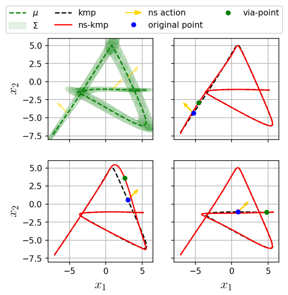
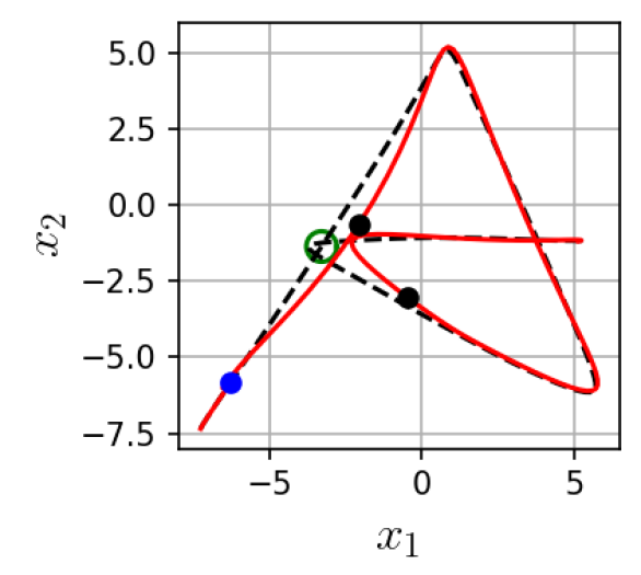
Unlike the robot control case, where regularization typically appears as a diagonal matrix, $\bm{\Sigma}_{n}$ are full covariance matrices. As a consequence, a null space reference generally does not affect all dimensions of the trajectory equally. The covariance at a given point influences both the magnitude and the directions along which a null space reference can modulate the trajectory. Figure 1 illustrates this property. The top-left image shows a trajectory distribution in 2D computed from examples of drawing a letter ‘A’ [29]. That distribution was used as a reference trajectory distribution in a KMP. Notice how the covariance changes throughout the trajectory. In the top-right and bottom images, we show the effect of applying a null space reference (yellow arrow), with the same magnitude, at different points along the trajectory. The dashed line is computed from (5) and the solid, red one from (15). The covariance in the null space projector constrains the modulated trajectory to deform less (more) along the directions where the variance is lower (higher). Additionally the modulation is applied along the axes of $\bm{\Sigma}_{n}$. This provides a principled way to use the variations in the original dataset to design optimal exploration strategies. Moreover, unlike typical exploration strategies that require the re-computation of model parameters or computationally costly operations to include new points in the trajectory, here adding new points is done inexpensively with (15). Indeed, the parameter $\bm{\Psi}$, that contains a potentially large matrix inverse operation, is computed only once from the reference trajectory distribution.

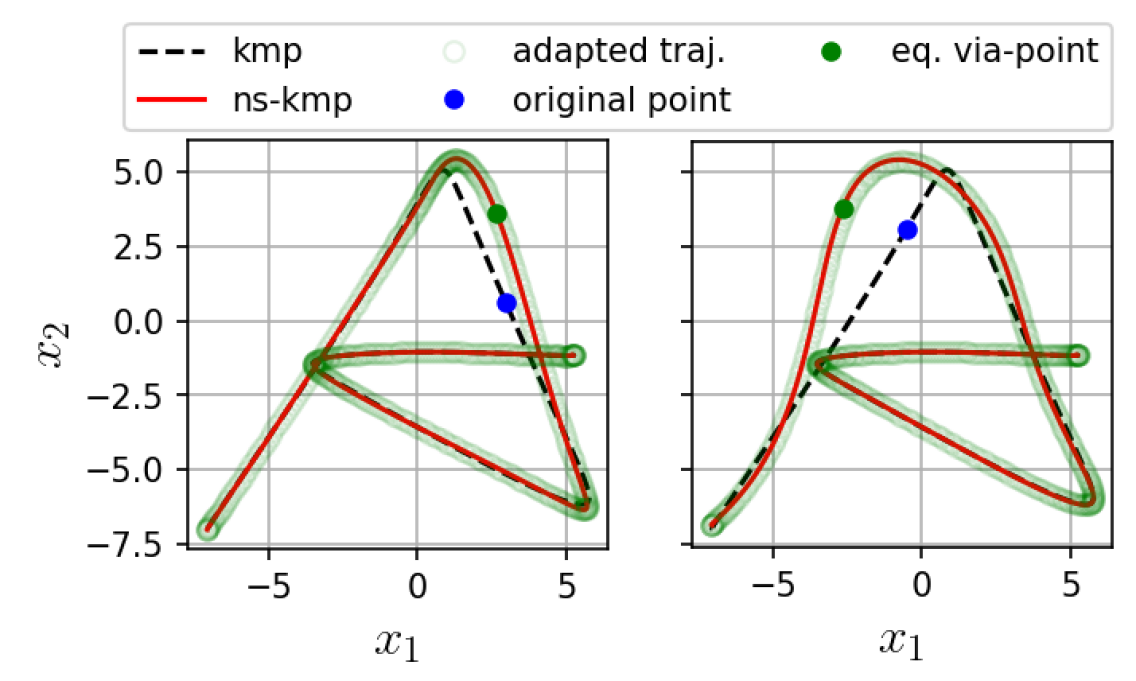
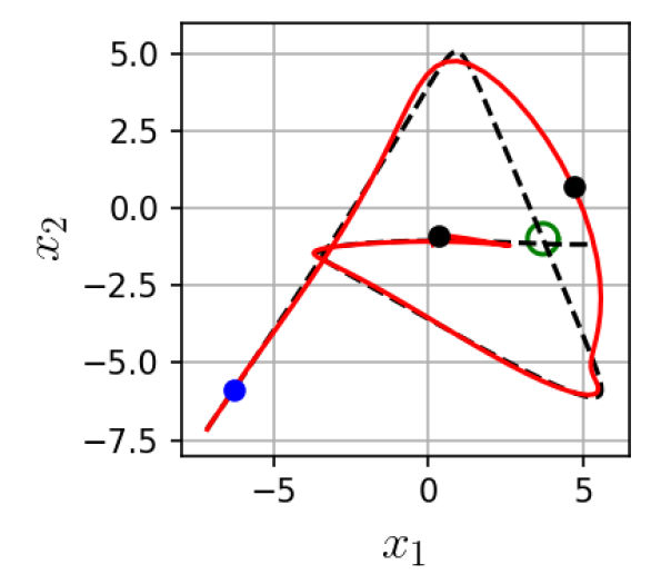
An important final property of NS-KMP is that null space modulation is equivalent to classical KMP modulation [14] given the appropriate via-point. For the sake of the explanation let us consider an input $\hat{\bm{s}}$ where a null space reference $\hat{\bm{\xi}}$ was applied, resulting in an observation $\bm{\xi}(\hat{\bm{s}})\neq\hat{\bm{\xi}}$ after the null space projector. We have concluded empirically that by treating the pair $\{\hat{\bm{s}},\bm{\xi}(\hat{\bm{s}})\}$ as a via-point in the classical KMP framework [14], and adding it to the reference trajectory distribution with a low covariance, generates the same trajectory as the null-space-generated one. Figure 2 illustrates this property. This result suggests that NS-KMP is, indeed, a computationally-efficient tool for via-point-based motion adaptation.

We use the handwritten letter dataset available in [29], particularly the dataset for letter ‘A’, to generate a trajectory distribution from demonstrations. It contains 10 demonstrations with time $t$ and 2D position $(x_{1},x_{2})$, which we use to train a mixture model with 8 components and retrieve a reference trajectory distribution $\{\bm{\mu}_{n},\bm{\Sigma}_{n}\}_{n=1}^{100}$ using Gaussian mixture regression. Moreover $\bm{s}=t$ and $\bm{\xi}=\left[x_{1}\>x_{2}\right]^{\top}$. In both KMP and NS-KMP implementations we use hyperparameters $\lambda=0.1$, $l=0.125$ while for ProMP we use 20 basis functions. The implementation was done in Python 3.8 running on an 8-core 11-Gen Intel Core i7-11850H @ 2.50GHz processor.

We use the learned models to simulate a robot planning a trajectory within a finite-horizon. At time $t$, the robot uses KMP, NS-KMP or ProMP to compute a trajectory for the horizon $\{t,\ldots,T\}$. We use $T=1$ with $10ms$ increments between time steps. At a randomly chosen time instant in the horizon, an obstacle (a circle with radius 0.5) with position uniformly sampled from $\{\bm{\mu}_{n}\}_{n=1}^{N}$ appears (only once) along the planned path. The robot then tests alternative paths looking for one that does not collide with the obstacle. In NS-KMP, this is done by sampling values of input $\hat{\bm{s}}$ and null space reference $\hat{\bm{\xi}}$ and computing the corresponding new trajectory using (15). The sampling interval for the input is $[t,\ldots,\mathrm{min}(t+0.2,T-t)]$ and $[-1000,1000]$ for the two dimensions of $\hat{\bm{\xi}}$ (we discuss this range of values in Section VII). In KMP and ProMP, finding alternative paths is done by sampling via-points in the neighborhood of the obstacle and inputs in the same range as for NS-KMP. To efficiently perform the exploration, including sampling null space references and via-points we used TPE [30], particularly the implementation available in the Optuna package [31]. We define a simple objective function to minimize $f(\bm{X}_{pred})=c_{collision}(\bm{X}_{pred})+c_{cont}(\bm{X}_{pred})$ where $\bm{X}_{pred}$ is the sequence of 2D points in the planned trajectory and $c_{collision}$ and $c_{cont}$ are collision and continuity terms that receive values of 1000 if a collision happens in $\bm{X}_{pred}$ or the norm between any two consecutive points in $\bm{X}_{pred}$ exceeds the radius of the obstacle and 0 otherwise. The optimizer returns the first solution with zero cost.

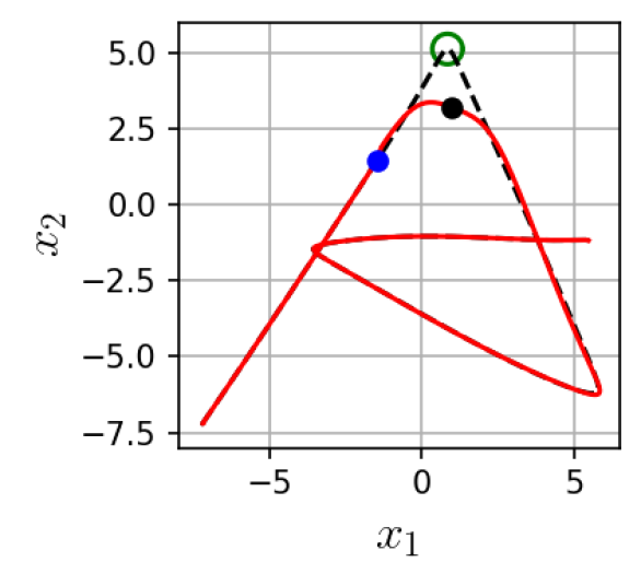
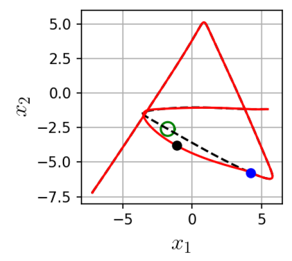
Figure 3(a) shows example trajectories obtained from NS-KMP. We observe that the obstacle is avoided correctly in different segments of the trajectory. Table I summarizes the time required by KMP, NS-KMP and ProMP to predict a trajectory from one null space reference or via-point (first row) and to find a solution to avoid the obstacle (second row). Each entry corresponds to the mean and standard deviation of 40 points. In the case of NS-KMP one prediction corresponds to computing $\hat{\bm{k}}^{*}$, $\hat{\bm{K}}$ and (15). For KMP it is the time of computing new matrices $\bm{K}$, $\bm{k}^{*}$ and (5), including the inversion. For ProMP it is the time to evaluate the basis functions at the new input, recompute the weight distribution and use it to compute a new trajectory (see [8]). Note that in this experiment we did not allow obstacles to appear at points where the trajectory intersects with itself (see these cases in Fig. 3(b)) since they require two via-points. The prediction times show that the parametric model ProMP was the fastest, closely followed by our non-parametric NS-KMP. Moreover, we observed comparable times between NS-KMP and ProMP to find a good trajectory (second row, 1 via-point (s)), with KMP (first column) taking two orders of magnitude longer.

Finally we investigated modulation by more than one via-point. For this we focused on the cases where the obstacle appears at places where the trajectory intersects with itself (Fig. 3(b)). Given the high computational cost of KMP shown in V-B we compare NS-KMP and ProMP only. Figure 3(b) shows that NS-KMP is capable of avoiding obstacles by modulating the planned trajectory with two via-points. As seen in Table I, last row, NS-KMP and ProMP achieved times within the same order of magnitude, with a slight disadvantage to ProMP.

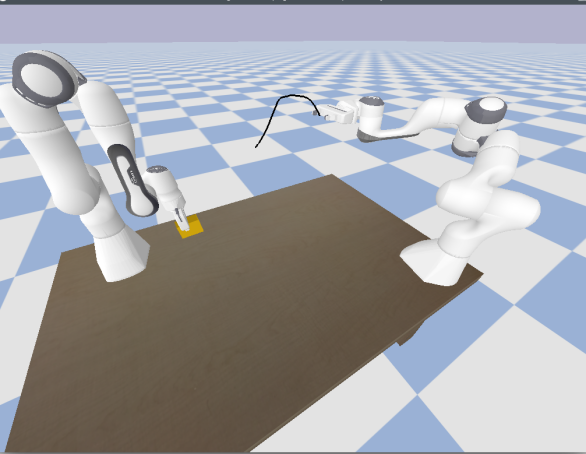
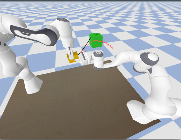
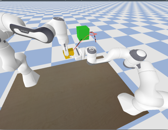
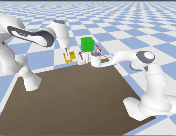
In order to train a NS-KMP we used the dataset collected from handover demonstrations in [32], with 5 demonstrations in the form of human hand and robot end-effector positions $\bm{x}_{H}$ and $\bm{x}_{R}$. The NS-KMP thus uses $\bm{s}=\bm{x}_{H}$ and $\bm{\xi}=\bm{x}_{R}$. In order to simulate the human-robot handover task, the data was rescaled to fit the robot workspaces in the pybullet setup depicted in Fig. 4. As illustrated in Fig. 4, the left robot plays the role that the human played in the demonstrations by picking up an object (yellow box) and handing it over to the robot on the right. The latter starts with a planned motion (black line) computed using as input the trajectory planned by the left robot (unavailable in a real scenario with a human, only shown for illustration). In each trial the motion is interrupted by a cube-shaped obstacle with an axial diagonal of $10cm$ that appears randomly (both in time and location) once along the black line. All the NS-KMP parameters were the same as in V. The optimization framework was also the same, however $\hat{\bm{\xi}}$ was sampled from the range $[-2000,2000]$ and the inputs (i.e. the left robot end-effector position) were sampled uniformly from the ones in the reference trajectory distribution. As in [14], we do not use ProMP as baseline here due to the difficulty in parameterizing basis functions for multi-dimensional inputs. Instead, we consider the optimization of Gaussian components in GMM as a baseline [6]. Specifically, we optimize the mean of one randomly chosen Gaussian until the collision cost is zero. We do not evaluate classical KMP in this section as the arguments that caused it to underperform in V-B are still valid (see also the analysis of computational complexity in Section VII-B).

In 20 trials, the average time to compute a solution with NS-KMP after the obstacle appears was $0.16s\pm 0.13$. Fig. 4, top-right and bottom, shows original and adapted trajectories. The GMM baseline yielded $0.616s\pm 0.571$.

The results in Section V revealed that our solution, despite not outperforming ProMP ($\approx 5\times$ faster at predicting), computes trajectories given a new desired point at the millisecond level (Table I, first row) with a non-optimized Python implementation. We believe this to be a noteworthy result for a non-parametric approach. Moreover, ProMP and NS-KMP performed at a similar level in finding a 1-via-point solution. However, ProMP is only $\approx 2.5\times$ faster, against $5\times$ for the individual prediction, suggesting that ProMP needs to try more via-points than NS-KMP to find a solution. This could be related to our choice of sampling via-points for ProMP around the obstacle, which may not be as efficient as the covariance-weighted exploration by NS-KMP. The reason for such choice is that we observed that the trajectories generated by ProMP often had arbitrary shapes (seriously violating the structure of the training data) if the search space of the via-point is not bounded or is large. The same reasoning applies to the 2-via-point case where NS-KMP took less time to find successful via-points.

Adaptation of learned multi-dimensional-input skills was a novelty introduced by KMP [14] and the results in Section VI show that NS-KMP provides a fast solution to adapting this type of skills. The GMM baseline was slower and the resulting trajectories were prone to distortions since only one Gaussian was being optimized at a time. The presented times for GMM can thus be seen as a lower bound since optimizing further parameters would require higher amounts of time. Despite the successful adaptation with NS-KMP we verified that, for our choice of hyperparameters, the time to compute a successful trajectory increases when the object appears closer to the handover location due to the decrease in variance (the null space ‘hardens’).

Some additional practical aspects of NS-KMP are worth discussing. As described in V–VI the magnitude of $\hat{\bm{\xi}}$ could be as high as 1000 or 2000 depending on the problem. Due to the probabilistic nature of the soft null space projector, one does not know a priori the required magnitude of $\hat{\bm{\xi}}$. It should thus be treated as a hyperparameter to be tuned depending on the problem. Additionally, while covariance-weighted null space exploration seems to alleviate the need to manually define exploration strategies, in some scenarios one might need to violate the priors imposed by the data, e.g. if the object has a much larger size. In other words it may be desirable to ‘soften’ the null space. This can be achieved by manually increasing $\lambda\bm{\Sigma}$, particularly in the neighborhood of the concerned region.

Classical KMP [14] predicts the expectation of $\bm{\xi}(\bm{s}^{*})$ using (5). When a new desired point described by the mean $\bar{\bm{\mu}}$ and covariance $\bar{\bm{\Sigma}}$ is needed, the reference trajectory distribution $\left\{\bm{\mu}_{n},\bm{\Sigma}_{n}\right\}^{N}_{n=1}$ is concatenated with $\{\bar{\bm{\mu}}$,$\bar{\bm{\Sigma}}\}$, leading to an extended reference trajectory with length $N+1$. Consequently, KMP needs to recompute the term $\left(\bm{K}+\lambda\bm{\Sigma}\right)^{-1}$ since the updated $\bm{\Sigma}$ includes $\bar{\bm{\Sigma}}$, see (3). Note that the dimension of $\bm{K}$ and $\bm{\Sigma}$ is $D(N+1)\times D(N+1)$ and therefore the computational complexity of classical KMP is $\mathcal{O}(D^{3}(N+1)^{3})$. Recall that in (15) we only search in the null space, where $\bm{K}$ remains the same and therefore $\bm{\Psi}$ can be computed beforehand in an offline fashion. Therefore, the computation complexity of (15) is $\mathcal{O}(D^{3}N^{2})$, which is significantly faster than classical KMP.

References

- [1] A. J. Ijspeert, J. Nakanishi, and S. Schaal, “Movement imitation with nonlinear dynamical systems in humanoid robots,” in Proc. IEEE Intl Conf. on Robotics and Automation (ICRA), 2002, pp. 1398–1403.
- [2] S. Calinon, F. Guenter, and A. Billard, “On learning, representing and generalizing a task in a humanoid robot,” IEEE Transactions on Systems, Man and Cybernetics, Part B. Special issue on robot learning by observation, demonstration and imitation, vol. 37, no. 2, pp. 286–298, 2007.
- [3] S. Calinon, “A tutorial on task-parameterized movement learning and retrieval,” Intelligent Service Robotics, vol. 9, no. 1, pp. 1–29, January 2016.
- [4] Y. Huang, J. Silvério, L. Rozo, and D. G. Caldwell, “Generalized task-parameterized skill learning,” in Proc. IEEE Intl Conf. on Robotics and Automation (ICRA), 2018, pp. 5667–5474.
- [5] F. Stulp and O. Sigaud, “Robot skill learning: From reinforcement learning to evolution strategies,” Paladyn, Journal of Behavioral Robotics, vol. 4, no. 1, pp. 49–61, 2013.
- [6] F. Guenter, M. Hersch, S. Calinon, and A. Billard, “Reinforcement learning for imitating constrained reaching movements,” Advanced Robotics, vol. 21, no. 13, pp. 1521–1544, 2007.
- [7] M. Saveriano, F. Franzel, and D. Lee, “Merging position and orientation motion primitives,” in Proc. IEEE Intl Conf. on Robotics and Automation (ICRA), 2019, pp. 7041–7047.
- [8] A. Paraschos, C. Daniel, J. Peters, and G. Neumann, “Probabilistic movement primitives,” in Advances in Neural Information Processing Systems (NIPS), 2013, pp. 2616–2624.
- [9] R. A. Shyam, P. Lightbody, G. Das, P. Liu, S. Gomez-Gonzalez, and G. Neumann, “Improving local trajectory optimisation using probabilistic movement primitives,” in Proc. IEEE/RSJ Intl Conf. on Intelligent Robots and Systems (IROS), 2019, pp. 2666–2671.
- [10] T. Löw, T. Bandyopadhyay, J. Williams, and P. V. Borges, “PROMPT: Probabilistic motion primitives based trajectory planning.” in Proc. Robotics: Science and Systems (R:SS), Virtual, July 2021.
- [11] M. Zucker, N. Ratliff, A. D. Dragan, M. Pivtoraiko, M. Klingensmith, C. M. Dellin, J. A. Bagnell, and S. S. Srinivasa, “CHOMP: Covariant hamiltonian optimization for motion planning,” The International Journal of Robotics Research, vol. 32, no. 9-10, pp. 1164–1193, 2013.
- [12] M. Kalakrishnan, S. Chitta, E. Theodorou, P. Pastor, and S. Schaal, “STOMP: Stochastic trajectory optimization for motion planning,” in Proc. IEEE Intl Conf. on Robotics and Automation (ICRA), 2011, pp. 4569–4574.
- [13] F. Frank, A. Paraschos, P. van der Smagt, and B. Cseke, “Constrained probabilistic movement primitives for robot trajectory adaptation,” IEEE Trans. on Robotics, vol. 38, no. 4, pp. 2276–2294, 2022.
- [14] Y. Huang, L. Rozo, J. Silvério, and D. G. Caldwell, “Kernelized movement primitives,” International Journal of Robotics Research, vol. 38, no. 7, pp. 833–852, 2019.
- [15] C. M. Bishop, Pattern Recognition and Machine Learning (Information Science and Statistics). Secaucus, NJ, USA: Springer, 2006.
- [16] G. Maeda, M. Ewerton, G. Neumann, R. Lioutikov, and J. Peters, “Phase estimation for fast action recognition and trajectory generation in human–robot collaboration,” The International Journal of Robotics Research, vol. 36, no. 13-14, pp. 1579–1594, 2017.
- [17] Y. Cui, J. Poon, J. V. Miro, K. Yamazaki, K. Sugimoto, and T. Matsubara, “Environment-adaptive interaction primitives through visual context for human–robot motor skill learning,” Autonomous Robots, vol. 43, no. 5, pp. 1225–1240, 2019.
- [18] J. Silvério, Y. Huang, L. Rozo, S. Calinon, and D. G. Caldwell, “Probabilistic learning of torque controllers from kinematic and force constraints,” in Proc. IEEE/RSJ Intl Conf. on Intelligent Robots and Systems (IROS), 2018, pp. 1–8.
- [19] J. Silvério, Y. Huang, L. Rozo, and D. G. Caldwell, “An uncertainty-aware minimal intervention control strategy learned from demonstrations,” in Proc. IEEE/RSJ Intl Conf. on Intelligent Robots and Systems (IROS), 2018, pp. 6065–6071.
- [20] C. E. Rasmussen and C. K. I. Williams, Gaussian processes for machine learning. Cambridge, MA, USA: MIT Press, 2006.
- [21] B. Siciliano and J.-J. Slotine, “A general framework for managing multiple tasks in highly redundant robotic systems,” in Fifth International Conference on Advanced Robotics ‘Robots in Unstructured Environments’, 1991, pp. 1211–1216.
- [22] C. W. Wampler, “Manipulator inverse kinematic solutions based on vector formulations and damped least-squares methods,” IEEE Transactions on Systems, Man, and Cybernetics, vol. 16, no. 1, pp. 93–101, 1986.
- [23] R. Mayorga, K. Ma, and A. Wong, “A robust local approach for the obstacle avoidance of redundant robot manipulators,” in Proc. IEEE/RSJ Intl Conf. on Intelligent Robots and Systems (IROS), vol. 3, 1992, pp. 1727–1734.
- [24] A. S. Deo and I. D. Walker, “Overview of damped least-squares methods for inverse kinematics of robot manipulators,” Journal of Intelligent and Robotic Systems, vol. 14, no. 1, pp. 43–68, 1995.
- [25] A. Dietrich, C. Ott, and A. Albu-Schäffer, “An overview of null space projections for redundant, torque-controlled robots,” The International Journal of Robotics Research, vol. 34, no. 11, pp. 1385–1400, 2015.
- [26] D.-H. Park, H. Hoffmann, P. Pastor, and S. Schaal, “Movement reproduction and obstacle avoidance with dynamic movement primitives and potential fields,” in Proc. IEEE Intl Conf. on Humanoid Robots (Humanoids), 2008, pp. 91–98.
- [27] Y. Huang, J. Silvério, L. Rozo, and D. G. Caldwell, “Hybrid probabilistic trajectory optimization using null-space exploration,” in Proc. IEEE Intl Conf. on Robotics and Automation (ICRA), Brisbane, Australia, May 2018, pp. 7226–7232.
- [28] M. Schneider and W. Ertel, “Robot learning by demonstration with local Gaussian process regression,” in Proc. IEEE/RSJ Intl Conf. on Intelligent Robots and Systems (IROS), 2010, pp. 255–260.
- [29] S. Calinon and D. Lee, Learning Control. Dordrecht: Springer Netherlands, 2019, pp. 1261–1312.
- [30] J. Bergstra, R. Bardenet, Y. Bengio, and B. Kégl, “Algorithms for hyper-parameter optimization,” in Advances in Neural Information Processing Systems (NIPS), J. Shawe-Taylor, R. Zemel, P. Bartlett, F. Pereira, and K. Weinberger, Eds., vol. 24. Curran Associates, Inc., 2011.
- [31] T. Akiba, S. Sano, T. Yanase, T. Ohta, and M. Koyama, “Optuna: A next-generation hyperparameter optimization framework,” in Proceedings of the 25rd ACM SIGKDD International Conference on Knowledge Discovery and Data Mining, 2019.
- [32] J. Silvério, Y. Huang, F. J. Abu-Dakka, L. Rozo, and D. G. Caldwell, “Uncertainty-aware imitation learning using kernelized movement primitives,” in Proc. IEEE/RSJ Intl Conf. on Intelligent Robots and Systems (IROS), 2019, pp. 90–97.
- [33] J. Vogel, A. Hagengruber, M. Iskandar, G. Quere, U. Leipscher, S. Bustamante, A. Dietrich, H. Hoppner, D. Leidner, and A. Albu-Schaffer, “EDAN: An EMG-controlled daily assistant to help people with physical disabilities,” in Proc. IEEE/RSJ Intl Conf. on Intelligent Robots and Systems (IROS), 2020, pp. 4183–4190.