A New Reduced Basis Method for Parabolic Equations Based on Single-Eigenvalue Acceleration
Abstract
In this paper, we develop a new reduced basis (RB) method, named as Single Eigenvalue Acceleration Method (SEAM), for second order parabolic equations with homogeneous Dirichlet boundary conditions. The high-fidelity numerical method adopts the backward Euler scheme and conforming simplicial finite elements for the temporal and spatial discretizations, respectively. Under the assumption that the time step size is sufficiently small and time steps are not very large, we show that the singular value distribution of the high-fidelity solution matrix is close to that of a rank one matrix. We select the eigenfunction associated to the principal eigenvalue of the matrix as the basis of Proper Orthogonal Decomposition (POD) method so as to obtain SEAM and a parallel SEAM. Numerical experiments confirm the efficiency of the new method.
Keywords: Reduced basis method; Proper orthogonal decomposition; Singular value; Second order parabolic equation
1 Introduction
The Reduced Basis (RB) method is a type of model order reduction approach for numerical approximation of problems involving repeated solution of differential equations generated in engineering and applied sciences. It was first proposed in [2] for the analysis of nonlinear structures in the 1970s, and later extended to many other problems such as partial differential equations (PDEs) with multiple parameters or different initial conditions [9, 4, 41, 10, 11, 37, 12, 39], PDE-constrained parametric optimization and control problems [16, 34, 17, 18], and inverse problems [24, 31]. It should be mentioned that the work in [38, 48] has led to a decisive improvement in the computational aspects of RB methods, owing to an efficient criterion for the selection of the basis functions, a systematic splitting of the computational procedure into an offline (parameter-independent) phase and an online (parameter-dependent) phase, and the use of posteriori error estimates that guarantee certified numerical solutions for the reduced problems. The RB methods that include the offline and online phases as their essential constituents have become the most widely used ones.
The Proper Orthogonal Decomposition (POD) method, combined with the Galerkin projection method, is a typical RB method. It uses a set of orthonormal bases, which can represent the known data in the sense of least squares, to linearly approximate the target variables so as to obtain a low-dimensional approximate model. Since it is optimal in the least square sense, the POD method has the property of completely relying, without making any a priori assumption, on the data.
The POD method, whose predecessor was initially presented by K.Pearson[36] in 1901 as an eigenvector analysis method and was originally conceived in the framework of continuous second-order processes by Berkooz[5], has been widely used in many fields with different appellations. In the singular value analysis and sample identification, the method is called the Karhumen-Loeve expansion [21]. In statistics it is named as the principal component analysis (PCA) [19]. In geophysical fluid dynamics and meteorological sciences, it is called the empirical orthogonal function method (EOF)[33, 42]. We can also see the widespread applications of POD method in fluid dynamics and viscous structures[3, 8, 15, 25, 35, 40, 43, 44, 45], optimal fluid control problems [20, 30], numerical analysis of PDEs [26, 22, 23, 1, 6, 27, 29, 28] and machine learning [32, 47, 13, 7, 46].
In this paper, we develop a new RB/POD method, named as Single Eigenvalue Acceleration Method (SEAM), for a full discretization, using backward Euler scheme for temporal discretization and continuous simplicial finite elements for spatial discretization, of second order parabolic equations with homogeneous Dirichlet boundary conditions. The idea of SEAM is inspired by a POD numerical experiment for a one-dimensional heat conduction problem:
| (1) |
When we focus on the numerical solution matrix of (1), where each column consists of the value of the numerical solution at a node, and the number of columns is the same as the number of time steps (We divide into 1000 equal parts and into 99 equal parts to get the high-fidelity numerical solution; see Figure 1), we observe something interesting: the principal singular value is much larger than other singular values of the numerical solution matrix! Here we recall that the singular values of are the arithmetic square roots of the eigenvalues of . Notice that when we use the POD method the choice of basis functions is often empirical. The observation tells us that we only need to choose one basis function when solving this equation with POD.
We show in Figure 1 , Figure 2 and Table 1 the SEAM (POD with one basis function) solution and computational details, respectively. We can see that when SEAM is used, the computational time can be saved greatly, and the relative error between the SEAM solution and the high-fidelity solution is very small.


| High-fidelity model | SEAM | ||
| Number of FEM d.o.fs (each time step) | 98 | Number of SEAM d.o.fs (each time step) | 1 |
| d.o.fs reduction | 98:1 | ||
| FE solution time | 1.73s | SEAM solution time | 762ms |
| SEAM-relative error in -norm | 1.2e-8 | ||
Based on the above observation from the numerical experiment of 1d case, we investigate SEAM for d-dimensional (d=2,3) second order parabolic problems with homogeneous Dirichlet boundary conditions. Under the assumption that the time step size is sufficiently small and the time steps are not very large, we show that the singular value distribution of the high-fidelity solution matrix is very close to a reference matrix of rank one. Then we select the eigenfunction associated to the principal eigenvalue as the POD basis so as to obtain SEAM.
The rest of the paper is arranged as follows. Section 2 introduces the model problem and its full discretization. Section 3 gives the SEAM algorithm and its parallel version. Section 4 discusses the singular value distribution of numerical solution matrix, and Section 5 reports some numerical experiments. Finally, Section 6 gives concluding remarks.
2 Model problem and fully discrete scheme
Let () be an open, bounded domain, and set for constant . We consider the following second-order parabolic problem: find such that
| (2) |
where with , , and and are given functions.
Let be a conforming shape-regular simplicial decomposition of the domain , and let be a space of standard finite elements of arbitrary order with respect to . Denote by the set of all interior nodes of , and by the nodal basis of with
Then we have
We divide the time interval into a uniform grid with nodes and step size for . For convenience we set for any function .
Let be the piecewise interpolation of . We consider the following fully discrete scheme for (2):
For , find such that
| (3) |
with initial data . Here denotes the -inner product on , and .
Introduce the numerical solution vector , the mass matrix , the total stiffness matrix , and the load vector , defined respectively by
Notice that and are both symmetric and positive definite. Since for a given the system (3) is of the matrix form
| (4) |
3 Single-Eigenvalue Acceleration Method
In this section, we give the SEAM algorithm, based on POD, and a parallel version. Let be the high-fidelity numerical solution vector defined by (4) for each , and let
| (5) |
be the numerical solution matrix of (2). Denote
| (6) |
and let
be the eigenvalues of , then the singular values of are
Set
Without loss of generality, we assume that . The POD method is to find the standard orthogonal basis functions of such that for any , , the mean square error between and its orthogonal projection onto the space is minimized on average, i.e.
| (7) |
A solution to (7) is called a POD-basis of rank .
We will show later (cf. Theorem 4.1 and Corollary 4.1) that the non-zero eigenvalues of except for the principal eigenvalue are close to zero if is not very large and the time step size is small enough. Based upon the theoretical result, we choose in the POD method (7). This means that we only need to use the biggest eigenvalue and the associated eigenvector to obtain the rank 1 POD basis (cf. [43])
For convenience, we name the POD method with as Single Eigenvalue Acceleration Method (SEAM), and the corresponding SEAM scheme for the full discretization (4) is as follows:
Given for the SEAM approximation solution at -th time step is obtained by
| (8) |
Note that the coefficients and in (8) are positive constants.
By Theorem 4.1 the model-order-reduction error of SEAM (8) is (cf. [39])
where is a positive constant independent of and . This means that the SEAM algorithm may be inaccurate when is not small enough. In other words, we can not expect the desired accuracy if is large. To overcome such a weakness, we will give a parallel SEAM below (cf. Remark 4.3).
For simplicity of notation, we assume . We divide the total numerical solution matrix as
with the submatrices
| (9) |
Then the parallel SEAM can be described as following:
Algorithm 1 Parallel SEAM
4 Singular Value Distribution of Numerical Solution Matrix
In this section, we apply a perturbation technique to investigate the singular value distribution of the numerical solution matrix in (5). We need the following result due to Hoffman and Wielandt [14]:
Lemma 4.1
If and are two symmetric matrices, then there hold
and
where are the eigenvalues of , and is the Frobenius norm of .
In what follows we assume that the time step is small enough such that
| (11) |
By noticing that is SPD, this assumption is reasonable.
Let represent the spectral radius of a matrix. As (11) implies , we have
| (12) |
In the case of , (10) is reduced to
| (13) |
Inspired by (12), for we define by
| (14) |
and define by
| (15) |
Denote
Remark 4.1
We easily see that the rank of is at most 1, which implies that has at most one non-zero singular value, and thus has at most one nonzero eigenvalue.
In the sequel we use to denote for simplicity, where is a generic positive constant independent of and and may be different at its each occurrence.
The following lemma shows that can be viewed as a perturbation of in some sense.
Lemma 4.2
Assume that is small enough such that (11) holds, then we have
| (16) |
Proof:
where
Thus,
| (17) | |||||
From the assumption (11) and the definitions of , , and , we have the following estimates:
and
Consequently, we obtain
which, together with (17), yields
Based on Lemma 4.2, we can get an error estimate between and :
Lemma 4.3
Assume that is small enough such that (11) holds, then we have
| (18) |
Proof:
| (19) |
Recalling that and we have
where
Then we obtain
By (11) it is easy to show that
As a result, we get
which, together with the triangle inequality and Lemma 4.2, yields the desired estimate.
Using Remark 4.1 and Lemmas 4.1 and 4.2, we immediately obtain the following main conclusion for the full discretization (10):
Theorem 4.1
Assume that is small enough such that (11) holds, then we have
| (20) |
This theorem directly yields the following result:
Corollary 4.1
Assume that is small enough such that (11) holds, and that for some , then we have
| (21) |
Remark 4.2
From Corollary 4.1, we can see that each singular value of the high-fidelity solution matrix is a small perturbation of the corresponding singular value of the reference matrix , provided that . Since has at most one non-zero singular value, all the singular values of , except for the largest one, are then close to zero.
Remark 4.3
From the analysis we know that Corollary 4.1 holds not only for , but also for with . This motivates the parallel SEAM in Section 3.
5 Numerical Results
This section provides some numerical experiments to verify the performance of SEAM for the fully discrete scheme (10) using continuous linear finite elements. All the tests are performed on a 12th-Gen Intel 3.20 GHz Core i9 computer.
5.1 Two-dimensional tests
We consider the following two-dimensional problem:
| (22) |
where and . To obtain the high-fidelity numerical solutions, we first divide the spatial domain uniformly into squares, then divide each square into isosceles right triangles. For the temporal subdivision, the coefficients , the initial data and the source term , we consider three situations:
-
S1:
, , , and ;
-
S2:
, , , , , and ;
-
S3:
, , , , , and .
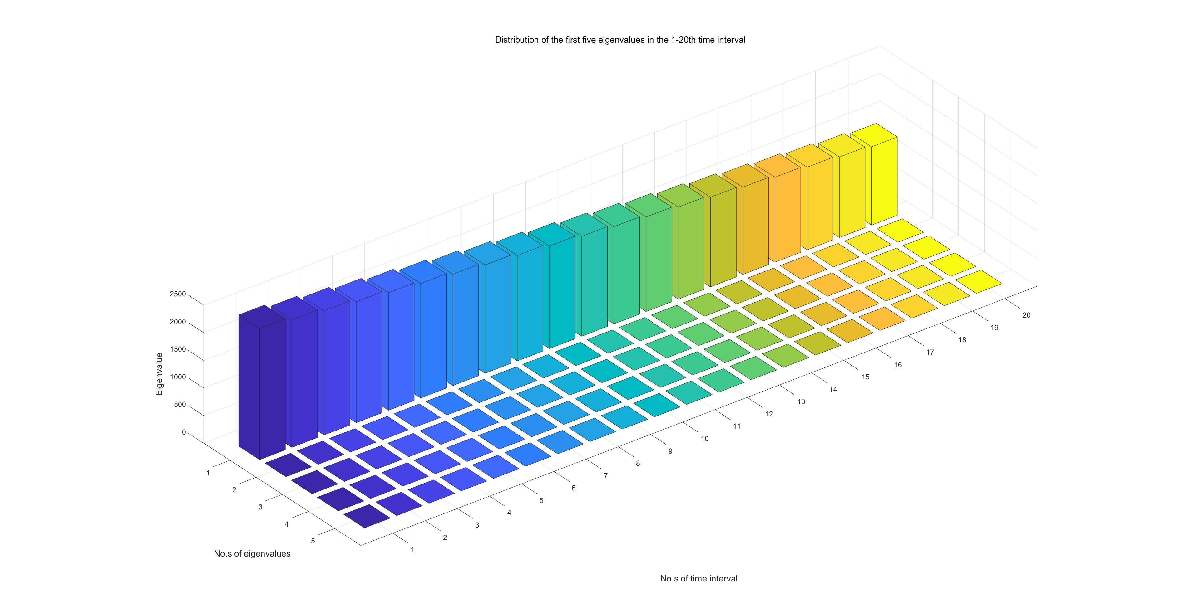
In S1 and S2, we take . In S3, we take . Figures 3 to 8 show the distribution of eigenvalues of for different in situations S1,S2 and S3, where the numerical solution matrix is defined by (9) for . In each figure, the label ’No.s of time interval’ means the time intervals, and the label ’No.s of eigenvalues’ means the first 5 eigenvalues in each time interval.
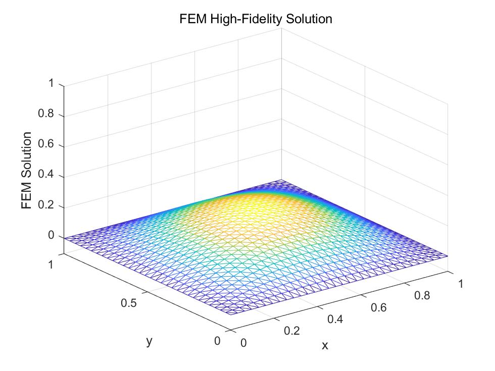
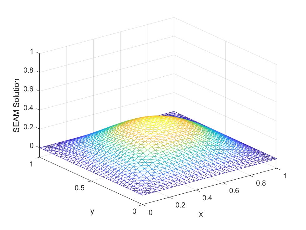
Figures 9 to 14 demonstrate the high-fidelity numerical solutions and the corresponding SEAM solutions of (22).
Tables 2 gives some computational details as well as the relative errors between the the SEAM solution and the high-fidelity numerical solution , with
From Figures 3 to 8, we have the following observations on the distribution of eigenvalues:
-
•
In each case the principal eigenvalue of is much larger than other eigenvalues. For example, in the case S2 with , for the first 100 steps, the principal eigenvalue is 2373.15 and the second largest one is 0.000256;
-
•
The eigenvalues of except the principal one are close to zero when and, though being not so close to zero, are still very small. These are consistent with Corollary 4.1;
-
•
As increases from to , the principal eigenvalues of gradually decrease. For example, in the case S1 with , the principal eigenvalues decrease from 3376.2 to 38.0. In the case S2 with , the principal eigenvalues decrease from 2389.5 to 1258.0. And in the case S3, the principal eigenvalues decrease from 4495.9 to 328.3.
From Figures 9 to 14 and Tables 2, we have the following observations on the SEAM solutions:
-
•
SEAM gives accurate numerical solutions for all cases;
-
•
SEAM is much faster than the original high-fidelity numerical method, due to the remarkable reduction of the size of the discrete model from to .


High-fidelity numerical solution


SEAM solution


High-fidelity numerical solution


SEAM solution


High-fidelity numerical solution


SEAM solution


High-fidelity numerical solution


SEAM solution


High-fidelity numerical solution


SEAM solution


High-fidelity numerical solution


SEAM solution
| High-fidelity model | SEAM | ||
| Number of FEM d.o.fs (each ) | Number of SEAM d.o.fs (each ) | ||
| d.o.fs reduction | |||
| FE solution time () | 8419s | SEAM solution time | 12s |
| FE solution time () | 8432s | SEAM solution time | 14s |
| FE solution time () | 8510s | SEAM solution time | 12s |
| FE solution time () | 8529s | SEAM solution time | 11s |
| FE solution time () | 8540s | SEAM solution time | 13s |
| FE solution time () | 301s | SEAM solution time | 3s |
| SEAM-Error() | |||
| SEAM-Error() | |||
| SEAM-Error() | |||
| SEAM-Error() | |||
| SEAM-Error() | |||
| SEAM-Error() | |||
5.2 A three-dimensional test
We consider the following three-dimensional problem:
| (23) |
where and . To obtain the high-fidelity numerical solution, we first divide the spatial domain uniformly into cubes, then divide each cube into tetrahedrons, and for the temporal subdivision we still take and in the full discretization (3).
Figure 15 shows the distribution of eigenvalues of , which is consistent with Corollary 4.1. Figure 16 shows the high-fidelity / SEAM solutions of (23), and Table 3 gives some computational details as well as the relative errors between the the SEAM solution and the high-fidelity numerical solution. We can see that the SEAM algorithm yields an accurate approximation solution and is much faster than the high-fidelity numerical method, due to the remarkable reduction of the size of the discrete model from to .


High-fidelity numerical solution


SEAM solution
| High-fidelity model | SEAM | ||
| Number of FEM d.o.fs (each ) | Number of SEAM d.o.fs (each ) | ||
| d.o.fs reduction | |||
| FE solution time | 40320s | SEAM solution time | 8s |
6 Conclusion
We have studied the singular value distribution of the numerical solution matrix corresponding to a full discretization of second order parabolic equations that uses the backward Euler scheme in time and continuous simplicial finite elements in space. Based on the property that the singular value distribution of the matrix formed by the high-fidelity solution is similar to a rank one matrix under the assumption that the time step size is sufficiently small, we have proposed the SEAM algorithm by choosing the eigenvector associated to the largest singular value as the POD basis. The resulting RB scheme at each time step is a linear equation with only one unknown. Numerical experiments have demonstrated the remarkable efficiency of SEAM.
7 Acknowledgement
This work was supported in part by the National Natural Science Foundation of China (12171340) and National Key R&D Program of China (2020YFA0714000).
References
- [1] D. Ahlman, F. Söderlund, J. Jackson, A. Kurdila, and W. Shyy, Proper orthogonal decomposition for time-dependent lid-driven cavity flows, Numerical Heat Transfer, Part B: Fundamentals, 42 (2002), pp. 285–306.
- [2] B. O. Almroth, P. Stern, and F. A. Brogan, Automatic choice of global shape functions in structural analysis, AIAA Journal, 16 (1978), pp. 525–528.
- [3] N. Aubry, P. Holmes, J. L. Lumley, and E. Stone, The dynamics of coherent structures in the wall region of a turbulent boundary layer, Journal of Fluid Mechanics, 192 (1988), pp. 115–173.
- [4] A. Barrett and G. Reddien, On the reduced basis method, ZAMM - Journal of Applied Mathematics and Mechanics / Zeitschrift für Angewandte Mathematik und Mechanik, 75 (1995), pp. 543–549.
- [5] G. Berkooz, Observations on the Proper Orthogonal Decomposition, Springer New York, New York, NY, 1992, pp. 229–247.
- [6] Y. Cao, J. Zhu, Z. Luo, and I. Navon, Reduced-order modeling of the upper tropical pacific ocean model using proper orthogonal decomposition, Computers & Mathematics with Applications, 52 (2006), pp. 1373–1386.
- [7] W. Chen, J. S. Hesthaven, B. Junqiang, Y. Qiu, Z. Yang, and Y. Tihao, Greedy nonintrusive reduced order model for fluid dynamics, AIAA Journal, 56 (2018), pp. 4927–4943.
- [8] D. T. Crommelin and A. J. Majda, Strategies for model reduction: Comparing different optimal bases, Journal of the Atmospheric Sciences, 61 (2004), pp. 2206–2217.
- [9] J. L. Eftang, D. J. Knezevic, and A. T. Patera, An hp certified reduced basis method for parametrized parabolic partial differential equations, Mathematical and Computer Modelling of Dynamical Systems, 17 (2011), pp. 395–422.
- [10] J. P. Fink and W. C. Rheinboldt, On the error behavior of the reduced basis technique for nonlinear finite element approximations, Zamm-zeitschrift Fur Angewandte Mathematik Und Mechanik, 63 (1983), pp. 21–28.
- [11] J. P. Fink and W. C. Rheinboldt, Solution manifolds and submanifolds of parametrized equations and their discretization errors, Numer. Math., 45 (1984), p. 323–343.
- [12] M. D. Gunzburger, Finite Element Methods for Viscous Incompressible Flows, Computer Science and Scientific Computing, Academic Press, San Diego, 1989.
- [13] J. Hesthaven and S. Ubbiali, Non-intrusive reduced order modeling of nonlinear problems using neural networks, Journal of Computational Physics, 363 (2018), pp. 55–78.
- [14] A. Hoffman and H. Wielandt, The variation of the spectrum of a normal matrix, Duke Math. J., 20 (1953), pp. 37–39.
- [15] P. Holmes, Turbulence, coherent structures, dynamical systems and symmetry, Cambridge University Press, 2012.
- [16] L. Iapichino, S. Ulbrich, and S. Volkwein, Multiobjective pde-constrained optimization using the reduced-basis method, Advances in Computational Mathematics, 43 (2017), pp. 945–972.
- [17] K. Ito and S. Ravindran, A reduced basis method for control problems governed by pdes, in Control and estimation of distributed parameter systems, Springer, 1998, pp. 153–168.
- [18] K. Ito and S. S. Ravindran, A reduced-order method for simulation and control of fluid flows, Journal of computational physics, 143 (1998), pp. 403–425.
- [19] I. T. Jolliffe, Principal component analysis, Springer, 2011.
- [20] R. D. Joslin, M. D. Gunzburger, R. A. Nicolaides, G. Erlebacher, and M. Y. Hussaini, Self-contained automated methodology for optimal flow control, AIAA Journal, 35 (1997), pp. 816–824.
- [21] F. Keinosuke, Introduction to Statistical Pattern Recognition, Academic Press, 2 ed., 1990.
- [22] Kunisch and Volkwein, Galerkin proper orthogonal decomposition methods for parabolic problems, Numerische Mathematik, 90 (2001), pp. 117–148.
- [23] Kunisch and Volkwein, Galerkin proper orthogonal decomposition methods for a general equation in fluid dynamics, SIAM Journal on Numerical Analysis, 40 (2002), pp. 492–515.
- [24] C. Lieberman, K. Willcox, and O. Ghattas, Parameter and state model reduction for large-scale statistical inverse problems, SIAM Journal on Scientific Computing, 32 (2010), pp. 2523–2542.
- [25] J. Lumley, Transition and Turbulence, Academic Press, 1981.
- [26] Z. Luo and G. Chen, Proper Orthogonal Decomposition Methods for Partial Differential Equations, Mathematics in Science and Engineering, Academic Press, 2019.
- [27] Z. Luo, J. Chen, J. Zhu, R. Wang, and I. M. Navon, An optimizing reduced order fds for the tropical pacific ocean reduced gravity model, International Journal for Numerical Methods in Fluids, 55 (2007), pp. 143–161.
- [28] Z. Luo, R. Wang, and J. Zhu, Finite difference scheme based on proper orthogonal decomposition for the nonstationary navier-stokes equations, Science in China Series A: Mathematics, 50 (2007), pp. 1186–1196.
- [29] Z. Luo, J. Zhu, R. Wang, and I. Navon, Proper orthogonal decomposition approach and error estimation of mixed finite element methods for the tropical pacific ocean reduced gravity model, Computer Methods in Applied Mechanics and Engineering, 196 (2007), pp. 4184–4195.
- [30] H. V. Ly and H. T. Tran, Proper orthogonal decomposition for flow calculations and optimal control in a horizontal cvd reactor, Quarterly of Applied Mathematics, 60 (2002), pp. 631–656.
- [31] Y. Maday, A. T. Patera, J. D. Penn, and M. Yano, A parameterized-background data-weak approach to variational data assimilation: formulation, analysis, and application to acoustics, International Journal for Numerical Methods in Engineering, 102 (2015), pp. 933–965.
- [32] L. Mainini and K. Willcox, Surrogate modeling approach to support real-time structural assessment and decision making, AIAA Journal, 53 (2015), p. 1612 – 1626. Cited by: 39.
- [33] A. J. Majda, I. Timofeyev, and E. Vanden-Eijnden, Systematic strategies for stochastic mode reduction in climate, Journal of the Atmospheric Sciences, 60 (2003), pp. 1705–1722.
- [34] A. Manzoni and S. Pagani, A certified rb method for pde-constrained parametric optimization problems, Communications in Applied and Industrial Mathematics, 10 (2019), pp. 123–152.
- [35] P. Moin and R. D. Moser, Characteristic-eddy decomposition of turbulence in a channel, Journal of Fluid Mechanics, 200 (1989), pp. 471–509.
- [36] K. Pearson, Liii. on lines and planes of closest fit to systems of points in space, Philosophical Magazine Series 1, 2, pp. 559–572.
- [37] J. S. Peterson, The reduced basis method for incompressible viscous flow calculations, SIAM Journal on Scientific and Statistical Computing, 10 (1989), pp. 777–786.
- [38] C. Prudhomme, D. V. Rovas, K. Veroy, L. Machiels, Y. Maday, A. T. Patera, and G. Turinici, Reliable Real-Time Solution of Parametrized Partial Differential Equations: Reduced-Basis Output Bound Methods , Journal of Fluids Engineering, 124 (2001), pp. 70–80.
- [39] A. Quarteroni, A. Manzoni, and F. Negri, Reduced Basis Methods for Partial Differential Equations An Introduction, Cham Springer International Publishing, 2016.
- [40] M. Rajaee, S. K. F. Karlsson, and L. Sirovich, Low-dimensional description of free-shear-flow coherent structures and their dynamical behaviour, Journal of Fluid Mechanics, 258 (1994), pp. 1–29.
- [41] W. C. Rheinboldt, On the theory and error estimation of the reduced basis method for multi-parameter problems, Nonlinear Analysis-theory Methods & Applications, 21 (1993), pp. 849–858.
- [42] F. M. Selten, Baroclinic empirical orthogonal functions as basis functions in an atmospheric model, Journal of the Atmospheric Sciences, 54 (1997), pp. 2099–2114.
- [43] Sirovich and Lawrence, Turbulence and the dynamics of coherent structures. Parts I-III., Quarterly of Applied Mathematics, 45 (1987), pp. 561–590.
- [44] Sirovich and Lawrence, Turbulence and the dynamics of coherent structures. ii. symmetries and transformations, Quarterly of Applied Mathematics, 45 (1987), pp. 573–582.
- [45] Sirovich and Lawrence, Turbulence and the dynamics of coherent structures. iii. dynamics and scaling, Quarterly of Applied Mathematics, 45 (1987), pp. 583–590.
- [46] R. Swischuk, L. Mainini, B. Peherstorfer, and K. Willcox, Projection-based model reduction: Formulations for physics-based machine learning, Computers & Fluids, 179 (2019), pp. 704–717.
- [47] E. Ulu, R. Zhang, and L. B. Kara, A data-driven investigation and estimation of optimal topologies under variable loading configurations, Computer Methods in Biomechanics and Biomedical Engineering: Imaging & Visualization, 4 (2016), pp. 61–72.
- [48] K. Veroy, C. Prud’homme, D. Rovas, and A. Patera, A posteriori error bounds for reduced-basis approximation of parametrized noncoercive and nonlinear elliptic partial differential equations, 16th AIAA Computational Fluid Dynamics Conference, (2003).