A New Least Squares Parameter Estimator for Nonlinear Regression Equations with Relaxed Excitation Conditions and Forgetting Factor
Abstract
In this note a new high performance least squares parameter estimator is proposed. The main features of the estimator are: (i) global exponential convergence is guaranteed for all identifiable linear regression equations; (ii) it incorporates a forgetting factor allowing it to preserve alertness to time-varying parameters; (iii) thanks to the addition of a mixing step it relies on a set of scalar regression equations ensuring a superior transient performance; (iv) it is applicable to nonlinearly parameterized regressions verifying a monotonicity condition and to a class of systems with switched time-varying parameters; (v) it is shown that it is bounded-input-bounded-state stable with respect to additive disturbances; (vi) continuous and discrete-time versions of the estimator are given. The superior performance of the proposed estimator is illustrated with a series of examples reported in the literature.
keywords:
Parameter estimation, Least squares identification algorithm, Nonlinear regression model, Exponentially convergent identification.1 Introduction
We have witnessed in the last few years an increasing interest in the analysis and design of new parameter estimators for linearly paramterized regression equations (LPRE) of the form , with measurable signals and a constant vector of unknown parameters.111We consider the case of scalar to simplify the notation—as will be seen below all results can be directly extended for the case of vector . The main motivation of this research is to relax the highly restrictive assumption of persistent excitation (PE) imposed to guarantee global exponential convergence of classical gradient, least squares (LS) or Kalman-Bucy algorithms [16, 48, 52]. A second important motivation is to provide guaranteed good transient performance behavior since the one of the aforementioned schemes is highly unpredictable and only a weak monotonicity property of the norm of the vector of estimation errors can be insured.
1.1 Review of recent literature on LS estimators
It has recently been shown [3, 43] that global asymptotic convergence—but not exponential—of the error equation for standard continous-time (CT) gradient estimators is ensured under a strictly weaker condition of generalized PE—see [3, 55] for its definition and [13] for some robustness properties of the algorithm. Unfortunately, this condition is still extremely restrictive to be of practical use. In [7] it is shown that the classical discrete-time (DT) LS algorithm is asymptotically convergent if and only if the regressor satisfies a new excitation property, called weak PE, that is strictly weaker than PE. This result is of limited interest because, on one hand, the definition is extremely technical and difficult to verify in applications. On the other hand, and more importantly, the analysis is limited to standard LS, without forgetting factor or covariance resetting that, as is well-known [16, 48], has a decreasing adaptation gain, loosing its alertness to track parameter variations, which is the main motivation for recursive algorithms. In [29] the underexcited scenario where the Gram matrix of the regressor has a -dimensional kernel, with , is considered. It is shown that incorporating into a CT LS (or gradient) estimator the information of a basis expanding this kernel—the columns of the matrix in equation (14) or (24) whose columns satisfy equation (4)—it is possible to guarantee consistent estimation to its complementary space. Clearly, if the regressor is PE the dimension of the aforementioned kernel is zero and convergence of all the parameters is guaranteed, confirming the well-known result of the PE case. This result is related to the partial convergence property of [48, Theorem 2.7.4] where a similar fact is proven in the context of systems identification in underexcited situations. Although of theoretical interest, the result has little practical relevance because of the impossibilty to compute on-line the matrix mentioned above. In [10] a slight modification of the DT LS algorithm is proposed to deal with parameter variations in the LPRE, however the main convergence (to a compact set) results still rely on PE assumptions. In [22], an LS version of the well-known I&I estimator [2] is proposed while in [28] a variation of LS that defines a passive operator is proposed.
In [49] an interesting generalization of the classical CT LS with forgetting factor is introduced, where the latter is allowed to be a time varying matrix. See [50] for a similar result in DT. The convergence analysis in both papers still relies on the PE assumption. In the very recent paper [5] a general structure to design and analyze DT LS-like recursive estimators parameterized in terms of some free functions is proposed—see equation (7). A new definition of excitation, called -excitation, is given in [5, Definition 1]. Interestingly, this definition involves not only the regressor but also two of the aforementioned functions. A particular choice of these functions yields the classical LS estimator and -excitation is equivalent to PE. However, other choices of these free parameters may yield weaker excitation conditions, for instance the choice given in (27). However, this selection has again the problem of driving the adaptation gain to zero, loosing the estimator alertness and it is not clear if there are other choices that do not suffer from this drawback. Another novelty of [5] is that it incorporates a very interesting analysis of robustness to additive disturbances in the LPRE, encrypted in the input-to-state-stability property. The interested reader is referred to [5, 49, 50] for a review of the extensive literature on LS with forgetting factors.
1.2 Relaxing the PE condition
A major breakthrough in the design of recurrent estimators is the proof that it is possible to establish global convergence under the extremely weak assumption of interval excitation222It should be pointed out that IE is strictly weaker than the generalized PE of [55], the weak excitation PE property of [7] and the -excitation of [5]. (IE) [20]—called initial excitation in [41] and excitation over a finite interval in [52]. To the best of the authors’ knowledge the first estimators where such a result was established are the concurrent and the composite learning schemes reported in [9] and [40], respectively; see [34] for a recent survey on new estimators. These algorithms, which incorporate the monitoring of past data to build a stack of suitable regressor vectors, are closer in spirit to off-line estimators. See also [19, 31] for two early references where a similar idea is explored. As is well-known, the main drawback of off-line estimators is their inability to track parameter variations, which is very often the main objective in applications. This situation motivates the interest to develop bona-fide on-line estimators that relax the PE condition preserving the scheme’s alertness [26].
New on-line estimators relying on the use of the dynamic regressor extension and mixing (DREM) technique with weaker excitation requirements have been recently proposed. DREM was first proposed in [1] for CT and in [4] for DT systems. In Appendix A it is recalled that the main step in the derivation of DREM estimators is the construction of a new extended LPRE , with and a new square matrix regressor. Two procedures to construct the extended LPRE, reported in [21] and [24], respectively, were originally considered—for the sake of completeness both constructions are reviewed in Appendix A. The final—and critical—mixing step consists of the multiplication of this extended LPRE by the adjugate of .333It is interesting to note that this operation was independently reported in [8] in the context of stochastic estimator convergence analysis. Clearly, this operation creates a new scalar LPRE of the form , with and a scalar regressor, which is the essential feature of the approach.444In Appendix A DREM is applied to nonlinearly parameterized regression equation (NLPRE) of the form (1), which is also considered in this paper. DREM estimators have been successfully applied in a variety of identification and adaptive control problems, both, theoretical and practical ones, see [34, 38] for an account of some of these results.
The convergence properties of DREM-based estimators clearly depend on the scalar regressor . Due to the scalar nature of , it is clear that the parameter error converges if and only if is not square integrable (summable for DT systems) and convergence is exponential if and only if is PE, facts that were proven in [1]. In [14] a DREM-based algorithm using the extended regressor of [21] that ensures convergence in finite-time imposing the IE assumption on was proposed. An interesting open question was to establish the relation of the excitation of and the original regressor , which was studied in [17] and [55] for the extended regressors of [21] and [24], respectively. The equivalence between PE of and PE of the original regressor was established for both extended regressors—proving that DREM-based estimators are at least as good as standard gradient or LS schemes for excited LPRE. On the other hand, in [17] it is shown that if is IE then is also IE for the extended regressor [21], while in [55] it was shown that the scheme of [24] ensures the stronger property that is bounded away from zero in an open interval with . Finally, in [38, Proposition 3] a new extended regressor which guarantees exponential convergence under conditions that are strictly weaker than regressor PE was presented.
Three major developments in this line of research reported recently are:
- (i)
-
(ii)
the proof in [53] that IE of the regressor is equivalent to identifiability of the LPRE. It should be recalled that identifiability of a LPRE is the existence of linearly independent regressor vectors [53, Definition 2] , and is a necessary and sufficient condition for the on- or off-line estimation of the parameters [16];
- (iii)
The estimators of [18] and [53] rely on the generation of new LPRE using the main idea of generalized parameter estimation based observer (GPEBO), which is a technique to design state observers for state-affine nonlinear systems, first proposed in [32] and latter generalized in [35]. GPEBO translates the problem of state-estimation into one of parameter estimation from a LPRE. The latter is generated exploiting the well-known property [47, Property 4.4] that the trajectories of an LTV system can be expressed as linear combinations of the columns of its fundamental matrix. Besides the addition of the computationally demanding calculation of the fundamental matrix, a potential drawback of GPEBO is that it essentially reconstructs the initial conditions of some error equation, an operation which may adversely affect the robustness of the estimator, [38, Remark 7] and [37], see also [54]. The procedure followed in the construction of the estimator of [18] is first the application of DREM and then invoke GPEBO, hence we refer to it as D+G. On the other hand, the estimator of [53] uses also GPEBO and DREM, but in the opposite order, so we refer to it in the sequel as G+D.
1.3 Contributions of the paper
In this paper we provide an alternative to the D+G and G+D estimators that also ensures global exponential convergence under the weak assumption of IE of the original regressor . The main features of this new estimator are summarized as follows.
F1 In contrast to the D+G and G+D estimators that implement a gradient descent search, we use the classical LS technique, hence we refer to it in the sequel as LS+D estimator. The superior convergence properties of LS estimators, as opposed to gradient-based, are widely recognized [16, 25, 45].
F2 We avoid the use of the GPEBO technique but instead exploit some structural properties of the LS estimator to construct the extended regressor. This fact removes the need to calculate the computationally demanding fundamental matrix.
F3 Similarly to the G+D scheme, the stability mechanism and, consequently, the stability analysis of the LS+D estimator is much more transparent than the one of the D+G estimator. There are two consequences of this fact, on one hand, the procedure of tuning the estimator to achieve a satisfactory transient performance, which is difficult for the D+G scheme, is straightforward for the LS+D one.
F4 A time-varying forgetting factor that allows the estimator to preserve its alertness to time-varying parameters is incorporated.
F5 Besides the case of LPRE we consider (separable and monotonic) NLPRE, with the associated estimator preserving all the properties of the case of LPRE. Also, we show that the proposed estimator is applicable to NLPRE with switched time-varying parameters.
F6 We show that the new estimator is robust with respect to additive disturbances, by proving that it defines a bounded-input-bounded-state (BIBS) stable system.
F7 The behaviour of many physical systems is described via CT models. On the other hand, DT implementations of estimators are of significant practical relevance. Therefore, similarly to [18, 38, 53], to comply with both scenarios we consider in the paper both kinds of LPREs. Interestingly, in contrast to [18], the construction and analysis tools of both cases are essentially the same—however, for the sake of clarity, they are presented in separate sections.
The remainder of the paper is organized as follows. In Section 2 we present the main result of the paper for CT systems, while the DT version is given in Section LABEL:sec3. For the sake of brevity we give both results for the general case of NLPRE, presenting the LPRE case as a corollary. Section 4 is devoted to the derivation of the proposed extended NLPRE applying directly the DREM construction procedure. Section 5 is devoted to the proof of robustness of the new estimator. Simulation results of some examples reported in the literature are given in Section 6 to illustrate the superior performance of the proposed LS+D estimator. The paper is wrapped-up with concluding remarks in Section 7.
Notation. is the identity matrix and is an matrix of zeros. , , and denote the positive and non-negative real and integer numbers, respectively. For we defined the set . For , we denote , and for any matrix its induced norm is . is an operator that piles up the columns of a matrix. CT signals are denoted , while for DT sequences we use , with the sampling time. The action of an operator on a CT signal is denoted as , and for a sequence .
2 Main Result for Continuous-time Systems
In this section we present the proposed LS+D interlaced estimator for CT systems, with the first estimator being the LS with bounded-gain forgetting factor proposed in [51, Subsection 8.7.6]. First, we consider the case of NLPRE and then specialize to LPRE that, as expected, ensures stronger convergence properties.
2.1 Nonlinearly parameterized regression equations
Consider the following CT NLPRE
| (1) |
where , and , a smooth mapping verifying the following.
Assumption A1. [Monotonicity] There exists a matrix such that mapping verifies the linear matrix inequality
| (2) |
for some . Consequently [12, 42], The mapping is strongly monotone, that is,
with .
Assumption A2. [Interval Excitation] The regressor is interval exciting (IE) [52, Definition 3.1]. That is, there exists constants and such that555In [52, Definition 3.1] there is an initial time in the integral that, for simplicity and without loss of generality, is taking here as zero.
| (3) |
Proposition 1.
Consider the NLPRE (1) with satisfying Assumption A1 and verifying Assumption A2. Define the LS+D interlaced estimator with time-varying forgetting factor
Assumption A3. [Lipschitz] The mapping satisfies the Lipschitz condition
| (4ein) |
for some .
Moreover, assume the regressor satisfies.
Assumption A4. [Interval Excitation] [52, Definition 3.3] The regressor is IE. That is, there exists constants and such that
| (4eip) |
Proposition 2.
Consider the NLPRE (LABEL:nlprek) with satisfying Assumption A1 and A3 and verifying Assumption A4. Define the normalized LS+DREM interlaced estimator
| (4eiqa) | |||
| (4eiqb) | |||
| (4eiqc) | |||
with initial conditions , and the definitions
| (4eiqra) | |||
with tuning parameters the initial condition , the forgetting factor and the adaptation gain , which is selected such that
| (4eiqrs) |
Define the parameter estimation error . Then, for all , and , we have that
| (4eiqrt) |
with all signals bounded.
Proof.
To simplify the notation we define the normalization sequence
| (4eiqru) |
With some abuse of notation, define the error signal
| (4eiqrv) |
whose dynamics is given by
where we used (LABEL:nlprek) and (LABEL:thegk). Now, direct application of the matrix inversion lemma to (4eiqb) shows that,
| (4eiqrw) |
Combining (LABEL:tileta) and (4eiqrw) we can prove the following fundamental property of LS
Solving this difference equation we get
where we replaced the solution of (4eiq) and the initial condition choice to get the second identity. Using the definition (4eiqrv), the equation above may be rewritten as the extended LPRE
Following the DREM procedure we multiply (LABEL:keyide) by to get the following NLPRE
| (4eiqrx) |
where we used (LABEL:delk) and (4eiqr). Replacing (4eiqrx) in (4eiqc) we get the dynamics of the parameter error
where, to simplify the notation, we defined the normalized scalar regressor sequence
| (4eiqry) |
To analyze the stability of this equation define the Lyapunov function candidate
| (4eiqrz) |
that satisfies
| (4eiqraa) | |||
| (4eiqrab) | |||
where we invoked Assumption A2 and Assumption A3 to get the first bound, (4eiqry) for the second one and used (4eiqrs) in the last identity. Summing the inequality above we get
Taking the limit as we conclude that , consequently
| (4eiqrac) |
Now, from the Algebraic Limit Theorem [46, Theorem 3.3] we know that the limit of the product of two convergent sequences is the product of their limits. On the other hand, from the fact that
we have that is a bounded monotonic sequence, hence it converges [46, Theorem 3.14]. Finally, if converges to a non-zero limit, we conclude from (4eiqrac) that .
We will proceed now to prove that (4eip) of Assumption A4 ensures this property of , which together with the fact that if converges to a non-zero limit, then also converges to a non-zero limit. Indeed, the solution of the difference equation (4eiqrw) is given by
Evaluating this expression for yields
The IE assumption ensures that the summation term is positive definite, since is nonsingular this ensures that the matrix on the left hand side is nonsingular. The proof that this property holds for any stems from the observation that, for any we have that
preserving the positivity property mentioned above. This completes the proof.
3.2 Linearly parameterized regression equations
In this section, we use the result of Proposition 2 for the case of LPRE—obviously, in this linear case Assumption A1 and Assumption A3 are automatically satisfied. As a first step we recall [53] that Definition LABEL:def1 and Lemma LABEL:lem1, given for continuous functions, are also valid for sequences.
As a second step notice that for the LPRE case (LABEL:keyide) takes the form
consequently (4eiqrx) now becomes
and the dynamics of the parameter error (LABEL:errequk) is now given by
whose stability is follows immediately from the IE assumption [53, Proposition 2] .
Corollary 2.
Consider the LPRE and assume it is identifiable. Define the normalized LS+D interlaced estimator with forgetting factor
with initial conditions , , tuning gains and , and we used the definitions (4eiqr). Then, for all , and , we have that (4eiqrac) holds with all signals bounded. Moreover, the individual parameter errors verify the monotonicity condition
Remark 2.
The importance of the element-by-element monotonicity property of the parameter error can hardly be overestimated. It played a key role for the relaxation of the assumption of known sign of the high frequency in model reference adaptive control [14, 53] as well as in the solution of the adaptive pole placement problem [44].
3.3 Switching parameters case
In this section, we consider the case of switched parameters estimation. Whereas the results are presented in DT only, similar results can be formulated for the CT case in a straightforward manner. Rewrite (LABEL:nlprek) as
| (4eiqrad) |
where denotes the switched unknown parameter vector with , , . The switching signal is a known777Such a scenario arises in several practical control scenarios, when the known switching signal characterizes known changes in operation regimes [23]. piecewise-constant function defining the behavior of , i.e., when , . The known time instants when changes its value are further denoted as , .
The estimator (4eiq), (4eiqr) is not capable of estimating switched parameters as for the sequence converges to zero, and for the LS estimator looses its alertness. To deal with switching parameters, we propose a resetting-based modification of the estimator (4eiq), (4eiqr):
| (4eiqraea) | ||||
| (4eiqraeb) | ||||
| (4eiqraec) | ||||
| (4eiqraed) | ||||
where , , and
| (4eiqrafa) | ||||
| (4eiqrafb) | ||||
Between the reseting instances , the estimator (4eiqrae), (4eiqraf) reproduces the estimator (4eiq), (4eiqr) with and thus . Then, at each reset instance , the matrix is reset to its initial condition , and the state saves the value of . The state thus plays the same role as in (LABEL:keyide), compare (4eiqrafb) and (4eiqr). Following the properties of (4eiq), (4eiqr), the proposed estimator ensures the boundedness of the states and is capable of estimating if the following assumption holds.
Assumption A5. [Switching Interval Excitation]. The switching signal is such that the regressor is IE between two subsequent switching instants. That is, there exist constants and such that for any
and
Remark 3.
In words, Assumption A5 means that the regressor satisfies the IE condition inside each subinterval . For simplicity we have taken that the constants and that appear in the definition of IE are the same for all subintervals , but this is clearly not necessary.
4 Derivation of the Extended NLPRE (LABEL:keyide1) via DRE
To simplify the reading of the material presented in this section we refer the reader to Appendix A where the procedure to derive DREM is recalled.
In Proposition 1 it is shown that the dynamic extension (LABEL:thegt1) and (LABEL:dotf) generates the extended NLPRE (LABEL:keyide1) to which we apply the mixing step S4 of Appendix A to generate the scalar NLPRE (LABEL:ydelc). In this section we prove that this extended NLPRE can also be derived directly applying the DREM step S2 of Appendix A for a suitably defined LTV operator .888We refer the interested reader to [53, Proposition 3] where the DREM operator for the G+D estimator reported in [53, Proposition 2] is identified. For the sake of brevity we only consider the CT case, with the DT case following verbatim.
Proposition 3.
Define the state space realization of the LTV operator used in step S2 of Appendix A as in (LABEL:dotu) with
with defined in (LABEL:dotf). Starting from the NLPRE , construct and via (2) that is, as the solutions of the dynamic extension
| (4eiqraga) | |||
and initial conditions and .
-
i)
The extended NLPRE holds.
-
ii)
The signals and satisfy (LABEL:ylsd) and (LABEL:philsd), respectively, with and solutions of the differential equations (LABEL:thegt1) and (LABEL:dotf), respectively.
Proof.
The fact that the extended NLPRE holds follows trivially from linearity of the operator .
To prove the claim (ii) we invoke (LABEL:ylsd) and do the following calculations
In the same spirit as above we compute the time derivative of as defined in (LABEL:philsd) to get
This completes the proof.
Remark 4.
Remark 5.
The dynamic extension (LABEL:dotf)and (4eiqrag) provides an alternative to the construction of the proposed estimator. The relationship between the two implementations boils down to a standard diffeomorphic change of coordinates. Indeed, while the state of the system in (4) and (LABEL:dotzet) is given by , the state of the system of Proposition 3 is , , and the first two components are related by a simple invertible coordinate change
However, the original implementation (4) clearly reveals the mechanism underlying the operation of the estimator, namely, the use of a classical LS update and the creation of the extended NLPRE exploiting the well-known property of LS (LABEL:prols).999To the best of the authors’ knowledge, this property was first reported in [11, equation (17)] and was widely used for the implementation of projections in indirect adaptive controllers [27].
5 Robustness Analysis of the CT LS+D Estimator
In this section we analyze the robustness vis-à-vis additive perturbations of the CT LS+D estimator of Proposition 1. That is, we consider the perturbed NLPRE
| (4eiqragah) |
where represents an additive perturbation signal. This signal may come from additive noise in the measurements of and or time variations of the parameters, that is, may be decomposed as
where and represent the measurement noise added to and , respectively, and captures time variations in the parameters. We make the reasonable assumption that these signals are all bounded and prove that the CT LS+D estimator defines a bounded-input-bounded-state (BIBS) stable system.
The main result is summarized in the proposition below.
Proposition 4.
Proof.
In the light of Remark 3, to carry out the proof we rely on the use of the alternative implementation of the extended NLPRE of Proposition 3. Applying the operator of Propositions 3 to the perturbed NLPRE (4eiqragah) yields the perturbed version of the extended LPRE (LABEL:extnlpre) as
| (4eiqragai) |
where we exploited the property of linearity of . Next we proceed to show that the operator is BIBO-stable. This is done by proving that, for all bounded , the signal is also bounded.
The signal is generated via the CT LTV system
Defining , we have
As and is bounded, this proves that , is also bounded.
From the analysis above, we conclude that the operator is BIBO-stable. Consequently, since and are bounded, it follows that and are also bounded. It only remains to prove that and is bounded. Whence, multiplying (4eiqragai) by we get the following perturbed NLPRE
| (4eiqragaj) |
where we defined the signal
| (4eiqragak) |
We notice that this signal is bounded. Replacing (4eiqragak) in the estimator (LABEL:thet1c) yields
Computing the derivative of the Lyapunov function candidate (LABEL:lyafunv) we get
The proof of boundedness of is completed recalling that in Proposition 1 it is shown that is PE.
6 Simulation Examples
In this section we present simulations of the proposed CT and DT estimators using different examples recently reported in the literature.
6.1 Example 5 of [29]
Consider the second order stable, CT, linear system described by
or equivalently
| (4eiqragal) |
where , and are unknown parameters. Applying the filter
where , to both sides of (4eiqragal) and rearranging the terms, we get the LPRE (LABEL:lrect) with
| (4eiqragam) |
and .
To carry out the simulations we use the same conditions that [29], that is, we set to zero the initial conditions of the filters, as well as the initial value of the parameter estimation vector , , and fix . Besides, the tuning parameters of the proposed estimator of Corollary LABEL:cor1 were , , and . In Fig. 1 we appreciate the transient behavior of the estimated parameters, which clearly shows the estimation of the real values. This result should be contrasted with the non-converging behavior of the estimates reported in [29] with the gradient scheme and their modified gradient.

To illustrate the use of the NLPRE (1), we notice that from the proposed values for , we have that can be rewritten as . Hence, after the application of the filter , the system (4eiqragal) can be written as the NLPRE (1) with , Thus, using the same initial conditions, estimator gains and verifying Assumption A1 with
and , we carry out a simulation to estimate only and with the estimator of Proposition 1. Fig. 2 shows the transient behavior of the estimated parameters, showing again parameter convergence.

6.2 Example 4 of [15]
Consider the first order linear system
| (4eiqragap) |
where is the forward-shiff operator and and are unknown parameters. After some simple calculations, we have that (4eiqragap) can be written as a LPRE with
To carry out the simulations we have also used the same initial conditions and parameters of [15], that is, , , and the input signal .101010We notice that there is an unfortunate typo in the definition of in [15, Example 4]. The tuning gains of the estimator of Corollary 2 were chosen as , , and initial conditions . It is important to note that for this system (4eiqragap), the estimator proposed in [15] only ensures the boundedness of , with (see Fig. 3 of [15]). This should be contrasted with our estimator, which, as can be seen in Fig. 3, converges to the real value.

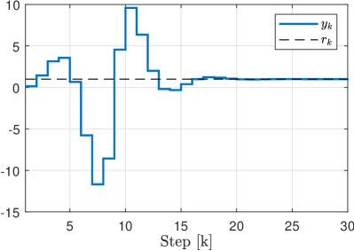
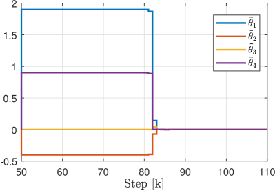
6.3 Example 8 of [30]
We consider the DT system
which switches for to
Note that for the plant is unstable and not minimum-phase. The initial conditions are , , and , and .
In this example, we consider the indirect adaptive poles placement for the reference tracking, where the reference signal is denoted as . Then the control signal is given by
where the time-varying coefficients , , , and are computed based on the current parameter estimate to provide the desired poles and unit gain of the closed-loop system; if for a value of the computations are ill-conditioned, then is chosen. For this example, the desired poles for this are , , and , and the reference signal is .
To estimate the parameters, we apply the resetting-based estimator (4eiqrae), (4eiqraf), where we set , , , and . Note that cannot be chosen zero as such a choice yields zero input to the system and the regressor is not IE; for a nonzero choice of , the interval excitation is provided by the transients of the plant.
The simulation results are depicted in Fig. 4 for the output signal and in Fig. 5 for the estimation errors . It can be observed that after the switch, parameters estimation errors remain almost constant for approximately steps, and then quickly converge. Further investigation shows that the regressor is not exciting on this initial interval, and thus the estimation does not progress. As soon as the IE condition is satisfied, the estimates converges to the true value .


7 Concluding Remarks
We have presented in this paper a new robust DREM-based parameter estimator that proves global exponential convergence of the parameter errors with the weakest excitation assumption, namely, identifiability of the LPRE—which is, actually necessary for the off- or on-line estimation of the parameters. The main features of the estimator are: (i) it relies on the use of a high performance LS search, in contrast to the usually slower gradient descents; (ii) it ensures component-wise monotonicity of the parameter estimation errors; (iii) it incorporates a forgetting factor avoiding the well-known covariance wind-up problem of LS; (iv) it is applicable to NLPRE, which are separable and monotonic as well as to switching parameters; (v) it constructs the extended regressor avoiding the use of the computationally demanding GPEBO technique, exploiting instead the key structural property of the LS estimator captured in (LABEL:prols); and (vi) CT and DT implementations of the estimator are given. Several simulation results, borrowed from the literature, show the superior performance of the proposed estimator.
Acknowledgments
The first author is grateful to Dr. Michelangelo Bin for a detailed explanation of his important results reported in [5] and to Prof. Han-Fu Chen for bringing to his attention the use of the mixing step of DREM in [8]. He also thanks Dr. Lei Wang for his help in the derivation of the CT version of the LS+D with a forgetting factor.
CRediT authorship contribution statement
All authors equally contributed to the paper.
References
- [1] S. Aranovskiy, A. Bobtsov, R. Ortega and A. Pyrkin, Performance enhancement of parameter estimators via dynamic regressor extension and mixing, IEEE Trans. Automatic Control, vol. 62, pp. 3546-3550, 2017.
- [2] A. Astolfi, D. Karagiannis and R. Ortega, Nonlinear and Adaptive Control with Applications, vol. 187, Springer, London, 2008.
- [3] N. E. Barabanov and R. Ortega, On global asymptotic stability of with bounded and not persistently exciting, Systems and Control Letters, vol. 109, pp. 24-27, 2017.
- [4] A. Belov, R. Ortega and A. Bobtsov, Guaranteed performance adaptive identification scheme of discrete-time systems using dynamic regressor extension and mixing, 18th IFAC Symposium on System Identification, (SYSID 2018), Stockholm, Sweden, July 9-11, 2018.
- [5] M. Bin, Generalized recursive least squares: Stability, robustness, and excitation, Systems & Control Letters, vol. 161, 105144, 2022.
- [6] A. Bobtsov, B. Yi, R. Ortega and A. Astolfi, Generation of new exciting regressors for consistent on-line estimation of a scalar parameter, IEEE Trans. Automatic Control, DOI: 10.1109/TAC.2022.3159568, 2022.
- [7] A. L. Bruce, A. Goel and D. S. Bernstein, Necessary and sufficient regressor conditions for the global asymptotic stability of recursive least squares, Systems & Control Letters, vol. 157, 10500527, 2021.
- [8] H. F. Chen and W. Zhao, Recursive Identification and Parameter Estimation, CRC Press, 2014.
- [9] G. Chowdhary, T. Yucelen, M. Muhlegg and E. N. Johnson, Concurrent learning adaptive control of linear systems with exponentially convergent bounds, International Journal of Adaptive Control and Signal Processing, vol. 27, no. 4, pp. 280-301, 2013.
- [10] Y. Cui, J. E. Gaudio and A. M. Annaswamy, A new algorithm for discrete-time parameter estimation, arXiv:2103.16653, 2021.
- [11] Ph. de Larminat, On the stabilizability condition in indirect adaptive control, Automatica, vol. 20, no, 6, pp. 793-795, 1984.
- [12] B. P. Demidovich, Dissipativity of nonlinear systems of differential equations, Vestnik Moscow State University, Ser. Mat. Mekh., Part I-6, (1961) pp. 19-27; Part II-1, (1962), pp. 3-8, (in Russian).
- [13] D. Efimov, N. Barabanov and R. Ortega, Robustness of linear time-varying systems with relaxed excitation, Int. J. on Adaptive Control and Signal Processing, vol. 33, no. 12, pp. 1885-1900, 2019.
- [14] D. Gerasimov, R. Ortega and V. Nikiforov, Adaptive control of multivariable systems with reduced knowledge of high frequency gain: Application of dynamic regressor extension and mixing estimators, 18th IFAC Symposium on System Identification, (SYSID 2018), Stockholm, Sweden, July 9-11, 2018.
- [15] A. Goel, A. L. Bruce and D. S. Bernstein, Recursive least squares with variable-direction forgetting: Compensating for the loss of persistency, IEEE Control Systems Magazine, vol. 40, no, 4, pp. 80-102, 2020.
- [16] G. Goodwin and K. Sin, Adaptive Filtering Prediction and Control, Prentice-Hall, 1984.
- [17] M. Korotina, S. Aranovskiy, R. Ushirobira and A. Vedyakov, On parameter tuning and convergence properties of the DREM procedure, 2020 European Control Conference (ECC20), Saint Petersburg, Russia, May 12-15, 2020.
- [18] M. Korotina, J. G. Romero, S. Aranovskiy, A. Bobtsov and R. Ortega, Persistent excitation is unnecessary for on-line exponential parameter estimation: a new algorithm that overcomes this obstacle, Systems & Control Letters, vol. 159, doi.org/10.1016/j.sysconle.2021.105079, 2022.
- [19] J. Krause and P. Khargonekar, Parameter information content of measurable signals in direct adaptive control, IEEE Trans. on Automatic Control, vol. 32, no. 9, pp. 802-810. 1987.
- [20] G. Kreisselmeier and G. Rietze-Augst, Richness and excitation on an interval—with application to continuous-time adaptive control, IEEE Trans. Automatic Control, vol. 35, no. 2, pp. 165-171, 1990.
- [21] G. Kreisselmeier, Adaptive observers with exponential rate of convergence, IEEE Trans. Automatic Control, vol. 22, no. 1, pp. 2-8, 1977.
- [22] M. Krstic, On using least-squares updates without regressor filtering in identification and adaptive control of nonlinear systems, Automatica, vol. 45, pp. 731-735, 2009.
- [23] D. Liberzon, Switching in Systems and Control, vol 190, Springer, 2003.
- [24] P.M. Lion, Rapid identification of linear and nonlinear systems, AIAA Journal, vol. 5, pp. 1835-1842, 1967.
- [25] L. Ljung, System Identification: Theory for the User, Prentice Hall, New Jersey, 1987.
- [26] L. Ljung and T. Soderstrom, Theory and Practice of Recursive Identification, MIT Press, 1983.
- [27] R. Lozano and X. Zhao, Adaptive pole placement without excitation probing signals, IEEE Trans. Automatic Control, vol. 39, no. 1, pp. 47-58, 1994.
- [28] R. Lozano and C. Canudas, Passivity-based adaptive control of mechanical manipulators using LS-type estimation, IEEE Trans. Automatic Control, vol. 35, no. 12, pp. 1363-1365, 1990.
- [29] R. Marino and P. Tomei, On exponentially convergent parameter estimation with lack of persistency of excitation, Systems & Control Letters, vol. 159, 105080, 2022.
- [30] T. Nguyen, S. Islam, D. Bernstein and I. Kolmanovsky, Predictive cost adaptive control: A numerical investigation of persistency, consistency, and exigency, IEEE Control Systems Magazine, vol. 41, pp. 64-96, 2021.
- [31] R. Ortega, An on-line least-squares parameter estimator with finite convergence time, Proc. IEEE, vol. 76, no. 7, 1988.
- [32] R. Ortega, A. Bobtsov, A. Pyrkin and S. Aranovskiy, A parameter estimation approach to state observation of nonlinear systems, Systems and Control Letters, vol. 85, pp 84-94, 2015.
- [33] R. Ortega, D. Gerasimov, N. Barabanov and V. Nikiforov, Adaptive control of linear multivariable systems using dynamic regressor extension and mixing estimators: Removing the high-frequency gain assumption, Automatica, vol. 110, 108589, 2019.
- [34] R. Ortega, V. Nikiforov and D. Gerasimov, On modified parameter estimators for identification and adaptive control: a unified framework and some new schemes, Annual Reviews in Control, vol. 50, pp. 278-293, 2020.
- [35] R. Ortega, A. Bobtsov, N. Nikolayev, J. Schiffer and D. Dochain, Generalized parameter estimation-based observers: Application to power systems and chemical-biological reactors, Automatica, vol. 129, 109635, 2021.
- [36] R. Ortega, V. Gromov, E. Nuño, A. Pyrkin and J. G. Romero, Parameter estimation of nonlinearly parameterized regressions: application to system identification and adaptive control, Automatica, vol. 127, 109544, 2021.
- [37] R. Ortega, Comments on recent claims about trajectories of control systems valid for particular initial conditions, Asian Journal of Control, DOI: 10.1002/asjc.2512, 2021.
- [38] R. Ortega, S. Aranovskiy, A. Pyrkin, A Astolfi and A. Bobtsov, New results on parameter estimation via dynamic regressor extension and mixing: Continuous and discrete-time cases, IEEE Trans. Automatic Control, vol. 66, no. 5, pp. 2265-2272, 2021.
- [39] R. Ortega, A. Bobtsov and N. Nikolayev, Parameter identification with finite-convergence time alertness preservation, IEEE Control Systems Letters, vol. 6, pp. 205-210, 2022
- [40] Y. Pan and H. Yu, Composite learning robot control with guaranteed parameter convergence, Automatica, vol. 89, pp. 398-406, 2018.
- [41] Y. Pan, S. Aranovskiy, A. Bobtsov, and H. Yu, Efficient learning from adaptive control under sufficient excitation, International Journal of Robust and Nonlinear Control, vol. 29, pp. 3111-3124, 2019.
- [42] A. Pavlov, A. Pogromsky, N. van de Wouw and H. Nijmeijer, Convergence dynamics, a tribute to Boris Pavlovich Demidovich, Systems & Control Letters, vol. 52, pp. 257-261, 2004.
- [43] L. Praly, Convergence of the gradient algorithm for linear regression models in the continuous and discrete-time cases, Int. Rep. MINES ParisTech, Centre Automatique et Systèmes, December 26, 2017.
- [44] A. Pyrkin, R. Ortega, V. Gromov, A. Bobtsov and A. Vedyakov, A Globally convergent direct adaptive pole-placement controller for nonminimum phase systems with relaxed excitation assumptions, Int. J. on Adaptive Control and Signal Processing, vol. 33, pp 1491-1505, 2019.
- [45] C. Rao and H. Toutenburg, H, Linear Models: Least Squares and Alternatives, Springer Series in Statistics (3rd ed.). Berlin, Springer, 2008.
- [46] W. Rudin, Principes of Mathematical Analysis, 3rd ed., NY:McGraw-Hill, Inc, 1976.
- [47] W.J. Rugh, Linear Systems Theory, 2nd ed., Prentice hall, NJ, 1996.
- [48] S. Sastry and M. Bodson, Adaptive Control: Stability, Convergence and Robustness, Prentice-Hall, New Jersey, 1989.
- [49] V. Shaferman, M. Schwegel, T. Gluck and A. Kugi, Continuous-time least-squares forgetting algorithms for indirect adaptive control, European Journal of Control, vol. 62, pp.105-112, 2021.
- [50] H. Shin and H. Lee, A new exponential forgetting algorithm for recursive least-squares parameter estimation, arXiv:2004.03910, 2020.
- [51] J.-J. E. Slotine and W. Li, Applied Nonlinear Control, Prentice-Hall, New Jersey, USA, 1991.
- [52] G. Tao, Adaptive Control Design and Analysis, vol. 37, John Wiley & Sons, New Jersey, 2003.
- [53] L. Wang, R. Ortega, A. Bobtsov, J. G. Romero and B. Yi, Identifiability implies robust, globally exponentially convergent on-line parameter estimation: Application to model reference adaptive control, arXiv:2108.08436, 2021.
- [54] Z. Wu, M. Ma, X. Xu, B. Liu and Z. Yu. Predefined-time parameter estimation via modified dynamic regressor extension and mixing, Journal of the Franklin Institute, doi.org/10.1016/j.jfranklin.2021.06.028, 2021.
- [55] B. Yi and R. Ortega, Conditions for convergence of dynamic regressor extension and mixing parameter estimators using LTI filters, IEEE Trans. Automatic Control, 10.1109/TAC.2022.3149964, 2022.
Appendix A
In this appendix we briefly review the main steps in the construction of DREM-based estimators proceeding from the NLPRE (1). For the sake of brevity we restrict ourselves to CT versions, with the DT ones constructed verbatim. The interested reader is refered to [38] for further details on these constructions.
Derivation of classical DREM-based estimators
-
S1
Starting from the NLPRE , with measurable signals, and a constant vector of unknown parameters.
-
S2
(Creation of the extended regressor) Inclusion of a free, stable, linear operator , with and , via its state space realization
with . Upon application to the NLPRE above, create a new extended NLPRE
(4eiqragat) with
We underscore the fact that the new extended regressor is a square matrix.
-
S3
For Kreisselmeier RE we select LTV operators with
-
S4
(Mixing step) Multiplication of the extended LPRE (4eiqragat) by the adjugate of to create the new NLPRE
(4eiqragau) with
and scalar regressor . Notice that in the case of LPRE we obtain scalar LPREs of the form