This paper was converted on www.awesomepapers.org from LaTeX by an anonymous user.
Want to know more? Visit the Converter page.

A New Initialization Technique for Reducing the Width of Neural Networks

Alexander Munteanu Dortmund Data Science Center, Faculties of Statistics and Computer Science, TU Dortmund University, Dortmund, Germany. Email: [email protected].    Simon Omlor Faculty of Statistics, TU Dortmund University, Dortmund, Germany. Email: [email protected].    Zhao Song Adobe Research. Email: [email protected].    David P. Woodruff Department of Computer Science, Carnegie Mellon University, Pittsburgh, PA 15213, USA. Email: [email protected].

Bounding the Width of Neural Networks via Coupled Initialization - A Worst Case Analysis

Alexander Munteanu Dortmund Data Science Center, Faculties of Statistics and Computer Science, TU Dortmund University, Dortmund, Germany. Email: [email protected].    Simon Omlor Faculty of Statistics, TU Dortmund University, Dortmund, Germany. Email: [email protected].    Zhao Song Adobe Research. Email: [email protected].    David P. Woodruff Department of Computer Science, Carnegie Mellon University, Pittsburgh, PA 15213, USA. Email: [email protected].
Abstract

A common method in training neural networks is to initialize all the weights to be independent Gaussian vectors. We observe that by instead initializing the weights into independent pairs, where each pair consists of two identical Gaussian vectors, we can significantly improve the convergence analysis. While a similar technique has been studied for random inputs [Daniely, NeurIPS 2020], it has not been analyzed with arbitrary inputs. Using this technique, we show how to significantly reduce the number of neurons required for two-layer ReLU networks, both in the under-parameterized setting with logistic loss, from roughly γ8\gamma^{-8} [Ji and Telgarsky, ICLR 2020] to γ2\gamma^{-2}, where γ\gamma denotes the separation margin with a Neural Tangent Kernel, as well as in the over-parameterized setting with squared loss, from roughly n4n^{4} [Song and Yang, 2019] to n2n^{2}, implicitly also improving the recent running time bound of [Brand, Peng, Song and Weinstein, ITCS 2021]. For the under-parameterized setting we also prove new lower bounds that improve upon prior work, and that under certain assumptions, are best possible.

1 Introduction

Deep learning has achieved state-of-the-art performance in many areas, e.g., computer vision LeCun et al. (1998); Krizhevsky et al. (2012); Szegedy et al. (2015); He et al. (2016), natural language processing Collobert et al. (2011); Devlin et al. (2018), self-driving cars, games Silver et al. (2016, 2017), and so on. A beautiful work connected the convergence of training algorithms for over-parameterized neural networks to kernel ridge regression, where the kernel is the Neural Tangent Kernel (NTK) Jacot et al. (2018).

The convergence results motivated by NTK mainly require two assumptions: (1) the kernel matrix KK formed by the input data points has a sufficiently large minimum eigenvalue λmin(K)λ>0\lambda_{\mathrm{min}}(K)\geq\lambda>0, which is implied by the separability of the input point set Oymak and Soltanolkotabi (2020), and (2) the neural network is over-parameterized. Mathematically, the latter means that the width of the neural network is a sufficiently large polynomial in the other parameters of the network, such as the number of input points, the data dimension, etc. The major weakness of such convergence results is that the neural network has to be sufficiently over-parameterized. In other words, the over-parameterization is a rather large polynomial, which is not consistent with architectures for neural networks used in practice, cf. Kawaguchi and Huang (2019).

Suppose mm is the width of the neural network, which is the number of neurons in a hidden layer, and nn is the number of input data points. In an attempt to reduce the number of neurons for binary classification, a recent work Ji and Telgarsky (2020) has shown that a polylogarithmic dependence on nn suffices to achieve arbitrarily small training error. Their width, however, depends on the separation margin γ\gamma in the RKHS (Reproducing Kernel Hilbert Space) induced by the NTK. More specifically they show an upper bound of m=O(γ8logn)m=O({\gamma^{-8}}{\log n}) and a lower bound of m=Ω(γ1/2)m=\Omega({\gamma}^{-1/2}) relying on the NTK technique. Our new analysis in this regime significantly improves the upper bound to m=O(γ2logn)m=O(\gamma^{-2}\log n).

We complement this result with a series of lower bounds. Without relying on any assumptions we show m=Ω(γ1)m=\Omega(\gamma^{-1}) is necessary. Assuming we need to rely on the NTK technique as in Ji and Telgarsky (2020), we can improve their lower bound to m=Ω(γ1logn)m=\Omega(\gamma^{-1}{\log n}). Finally, assuming we need to rely on a special but natural choice for estimating an expectation by its empirical mean in the analysis of Ji and Telgarsky (2020), which we have adopted in our general upper bound, we can even prove that m=Θ(γ2logn)m=\Theta(\gamma^{-2}{\log n}), i.e., that our analysis is tight. However, in the 22-dimensional case we can construct a better estimator yielding a linear upper bound of m=O(γ1logn)m=O({\gamma^{-1}}{\log n}), so the above assumption seems strong for very low dimensions, though it is a seemingly natural method that works in arbitrary dimensions. We also present a candidate hard instance in Θ(logγ1)\Theta(\log\gamma^{-1}) dimensions which could potentially give a matching Ω(γ2)\Omega(\gamma^{-2}) lower bound, up to logarithmic factors.

For regression with target variable yy with |y|O(1)|y|\in O(1) we consider a two-layer neural network with squared loss and ReLU as the activation function, which is standard and popular in the study of deep learning. Du et al. (2019c) show that m=O(λ4n6)m=O(\lambda^{-4}n^{6}) suffices (suppressing the dependence on remaining parameters). Further, Song and Yang (2019) improve this bound to m=O(λ4n4)m=O(\lambda^{-4}n^{4}). The trivial information-theoretic lower bound is Ω(n)\Omega(n), since the model has to memorize111Here, by memorize, we mean that the network has zero error on every input point. the nn input data points arbitrarily well. There remains a huge gap between nn and n4n^{4}. In this work, we improve the upper bound, showing that m=O(λ2n2)m=O(\lambda^{-2}n^{2}) suffices for gradient descent to get arbitrarily close to 0 training error. We summarize our results and compare with previous work in Table 1.

1.1 Related Work

The theory of neural networks is a huge and quickly growing field. Here we only give a brief summary of the work most closely related to ours.

Convergence results for neural networks with random inputs. Assuming the input data points are sampled from a Gaussian distribution is often done for proving convergence results Zhong et al. (2017b); Li and Yuan (2017); Zhong et al. (2017a); Ge et al. (2018); Bakshi et al. (2019); Chen et al. (2020). A more closely related work is the work of Daniely (2020) who introduced the coupled initialization technique, and showed that O~(n/d)\widetilde{O}(n/d) hidden neurons can memorize all but an ϵ\epsilon fraction of nn random binary labels of points uniformly distributed on the sphere. Similar results were obtained for random vertices of a unit hypercube and for random orthonormal basis vectors. In contrast to our work, this reference uses stochastic gradient descent, where the nice assumption on the input distribution gives rise to the 1/d1/d factor; however, this reference achieves only an approximate memorization. We note that full memorization of all input points is needed to achieve our goal of an error arbitrarily close to zero, and Ω(n)\Omega(n) neurons are needed for worst case inputs. Similarly, though not necessarily relying on random inputs, Bubeck et al. (2020) shows that for well-dispersed inputs, the neural tangent kernel (with ReLU network) can memorize the input data with O~(n/d)\widetilde{O}(n/d) neurons. However, their training algorithm is neither a gradient descent nor a stochastic gradient descent algorithm, and also their network consists of complex weights rather than real weights. One motivation of our work is to analyze standard algorithms such as gradient descent. In this work, we do not make any input distribution assumptions; therefore, these works are incomparable to ours. In particular, random data sets are often well-dispersed inputs that allow smaller width and tighter concentration, but are hardly realistic. In contrast, we conduct worst case analyses to cover all possible inputs, which might not be well-dispersed in practice.

Convergence results of neural networks in the under-parameterized setting. When considering classification with cross-entropy (logistic) loss, the analogue of the minimum eigenvalue parameter of the kernel matrix is the maximum separation margin γ\gamma (see Assumption  3.1 for a formal definition) in the RKHS of the NTK. Previous separability assumptions on an infinite-width two-layer ReLU network in Cao and Gu (2019b, a) and on smooth target functions in Allen-Zhu et al. (2019a) led to polynomial dependencies between the width mm and the number nn of input points. The work of Nitanda et al. (2019) relies on the NTK separation mentioned above and improved the dependence, but was still polynomial.

A recent work of Ji and Telgarsky (2020) gives the first convergence result based on an NTK analysis where the direct dependence on nn, i.e., the number of points, is only poly-logarithmic. Specifically, they show that as long as the width of the neural network is polynomially larger than 1/γ1/\gamma and logn\log n, then gradient descent can achieve zero training loss.

Convergence results for neural networks in the over-parameterized setting. There is a body of work studying convergence results of over-parameterized neural networks Li and Liang (2018); Du et al. (2019c); Allen-Zhu et al. (2019c, b); Du et al. (2019b); Allen-Zhu et al. (2019a); Song and Yang (2019); Arora et al. (2019b, a); Cao and Gu (2019b); Zou and Gu (2019); Du et al. (2019a); Lee et al. (2020); Huang and Yau (2020); Chen and Xu (2020); Brand et al. (2021); Li et al. (2021); Song et al. (2021). One line of work explicitly works on the neural tangent kernel Jacot et al. (2018) with kernel matrix KK. This line of work shows that as long as the width of the neural network is polynomially larger than n/λmin(K)n/\lambda_{\min}(K), then one can achieve zero training error. Another line of work instead assumes that the input data points are not too “collinear”, where this is formalized by the parameter δ=minij{xixj2,xi+xj2}\delta=\min_{i\neq j}\{\|x_{i}-x_{j}\|_{2},\|x_{i}+x_{j}\|_{2}\}222This is also sometimes called the separability of data points. Li and Liang (2018); Oymak and Soltanolkotabi (2020). These works show that as long as the width of the neural network is polynomially larger than 1/δ1/\delta and nn, then one can train the neural network to achieve zero training error. The work of Song and Yang (2019) shows that the over-parameterization m=Ω(λ4n4)m=\Omega(\lambda^{-4}n^{4}) suffices for the same regime we consider333Although the title of Song and Yang (2019) is quadratic, n2n^{2} is only achieved when the finite sample kernel matrix deviates from its limit in norm only by a constant α\alpha w.h.p., and the inputs are well-dispersed with constant θ\theta, i.e., |xi,xj|θ/n|\langle x_{i},x_{j}\rangle|\leq\theta/\sqrt{n} for all iji\neq j. In general, Song and Yang (2019) only achieve a bound of n4n^{4}. . Additional work claims that even a linear dependence is possible, though it is in a different setting. E.g., Kawaguchi and Huang (2019) show that for any neural network with nearly linear width, there exists a trainable data set. Although their width is small, this work does not provide a general convergence result. Similarly, Zhang et al. (2021) use a coupled LeCun initialization scheme that also forces the output at initalization to be 0. This is shown to improve the width bounds for shallow networks below nn neurons. However, their convergence analysis is local and restricted to cases where it remains unclear how to find globally optimal or even approximate solutions. We instead focus on cases where gradient descent provably optimizes up to arbitrary small error, for which we give a lower bound of Ω(n)\Omega(n).

Other than considering over-parameterization in first-order optimization algorithms, such as gradient descent, Brand et al. (2021) show convergence results via second-order optimization, such as Newton’s method. Their running time also relies on m=Ω(λ4n4)m=\Omega(\lambda^{-4}n^{4}), which is the state-of-the-art width for first-order methods Song and Yang (2019), and it was noted that any improvement to mm would yield an improved running time bound.

Our work presented in this paper continues and improves those lines of research on understanding two-layer ReLU networks.

Roadmap.

In Section 2, we introduce our problem formulations and present our main ideas. In Section 3, we present our main results. In Section 4, we present a technical overview of our core analysis for the convergence of the gradient descent algorithm in both of our studied regimes and give a hard instance and the intuition behind our lower bounds. In Section 5, we conclude our paper with a summary and some discussion.

We defer all detailed technical proofs to the appendix. The details for the logarithmic width networks under logistic loss are given in Appendices B-F, whereas the polynomial width networks with squared loss are analyzed in Appendices G-I.

2 Problem Formulation and Initialization Scheme

We follow the standard problem formulation Du et al. (2019c); Song and Yang (2019); Ji and Telgarsky (2020). One major difference of our formulation with the previous work is that we do not have a 1/m1/\sqrt{m} normalization factor in what follows. We note that only removing the normalization does not give any improvement in the amount of over-parameterization required of the previous bounds. The output function of our network is given by

f(W,x,a)=r=1marϕ(wrx),f(W,x,a)=\sum_{r=1}^{m}a_{r}\phi(w_{r}^{\top}x), (1)

where ϕ(z)=max{z,0}\phi(z)=\max\{z,0\} denotes the ReLU activation function444We note that our analysis can be extended to Lipschitz continuous, positively homogeneous activations., xdx\in\mathbb{R}^{d} is an input point, w1,,wmdw_{1},\ldots,w_{m}\in\mathbb{R}^{d} are weight vectors in the first (hidden) layer, and a1,,am{1,+1}a_{1},\ldots,a_{m}\in\{-1,+1\} are weights in the second layer. We only optimize WW and keep aa fixed, which suffices to achieve zero error. Also previous work shows how to extend the analysis to include aa in the optimization, cf. Du et al. (2019c).

Definition 2.1 (Coupled Initialization).

We initialize the network weights as follows:

  • For each r=2i1r=2i-1, we choose wrw_{r} to be a random Gaussian vector drawn from 𝒩(0,I)\mathcal{N}(0,I).

  • For each r=2i1r=2i-1, we sample ara_{r} from {1,+1}\{-1,+1\} uniformly at random.

  • For each r=2ir=2i, we choose wr=wr1w_{r}=w_{r-1}.

  • For each r=2ir=2i, we choose ar=ar1a_{r}=-a_{r-1}.

We note this coupled initialization appeared before in Daniely (2020) for analyzing well-spread random inputs on the sphere. The initialization is chosen in such a way as to ensure that for each of the nn input points, the initial value of the network is 0. Here we present an independent and novel analysis, where this property is leveraged repeatedly to bound the iterations of the optimization, which yields significantly improved worst case bounds for any input. This is crucial for our analysis, and is precisely what allows us to remove the 1/m1/\sqrt{m} factor that multiplies the right-hand-side of (1) in previous work. Indeed, that factor was there precisely to ensure that the initial value of the network is small. One might worry that our initialization causes the weights to be dependent. Indeed, each weight vector occurs exactly twice in the hidden layer. We are able to show that this dependence does not cause problems for our analysis. In particular, the minimum eigenvalue bounds of the associated kernel matrix and the separation margin in the NTK-induced feature space required for convergence in previous work can be shown to still hold, since such analyses are loose enough to accommodate such dependencies. Now, we have a similar initialization as in previous work, but since we no longer need a 1/m1/\sqrt{m} factor in (1), we can show that we can change the learning rate of gradient descent from that in previous work and it no longer needs to be balanced with the initial value, since the latter is 0. This ultimately allows for us to use a smaller over-parameterization (i.e., value of mm) in our analyses. For r[m]r\in[m], we have555Note that ReLU is not continuously differentiable. Slightly abusing notation, one can view f/wr\partial f/\partial w_{r} as a valid (sub)gradient given in the RHS of (2). This extends to L/wr\partial L/\partial w_{r} as the RHS of (4) and (5) which yields the update rule (6) commonly used in practice and in related theoretical work, cf. Du et al. (2019c).

f(W,x,a)wr=arx𝟏wrx0\displaystyle\frac{\partial f(W,x,a)}{\partial w_{r}}=a_{r}x{\bf 1}_{w_{r}^{\top}x\geq 0} (2)

independent of the loss function that we aim to minimize.

2.1 Loss Functions

In this work, we mainly focus on two different types of loss functions. The binary cross-entropy (logistic) loss and the squared loss. These loss functions are arguably the most well-studied for binary classification and for regression tasks with low numerical error, respectively.

We are given a set of nn input data points and corresponding labels, denoted by

{(x1,y1),,(xn,yn)}d×.\displaystyle\{(x_{1},y_{1}),\ldots,(x_{n},y_{n})\}\subset\mathbb{R}^{d}\times\mathbb{R}.

We make a standard normalization assumption, as in Du et al. (2019c); Song and Yang (2019); Ji and Telgarsky (2020). In the case of logistic loss, the labels are restricted to yi{1,+1}y_{i}\in\{-1,+1\}. In the case of squared loss, the labels are |yi|=O(1)|y_{i}|=O(1). In both cases, as in prior work and for simplicity, we assume that xi2=1\|x_{i}\|_{2}=1666 We adopt the assumption for a concise presentation, but we note it can be resolved by weaker constant bounds 0<lbxiub0<\mathrm{lb}\leq\|x_{i}\|\leq\mathrm{ub}, introducing a constant ub/lb\mathrm{ub}/\mathrm{lb} factor, cf. Du et al. (2019c), or otherwise the data can be rescaled and padded with an additional coordinate to ensure xi=1\|x_{i}\|=1, cf. Allen-Zhu et al. (2019a). , i[n]\forall i\in[n]. We also define the output function on input xix_{i} to be fi(W)=f(W,xi,a)f_{i}(W)=f(W,x_{i},a). At time tt, let u(W(t))=(u1(W(t)),,un(W(t)))nu(W(t))=(u_{1}(W(t)),\ldots,u_{n}(W(t)))\in\mathbb{R}^{n} be the prediction vector, where each ui(W(t))u_{i}(W(t)) is defined to be

ui(W(t))=f(W(t),xi,a).\displaystyle u_{i}(W(t))=f(W(t),x_{i},a). (3)

For simplicity, we use u(t)u(t) to denote u(W(t))u(W(t)) in later discussion.

We consider the objective function LL:

L(W)=i=1n(yi,ui(W))\displaystyle L(W)=\sum_{i=1}^{n}\ell(y_{i},u_{i}(W))

where the individual logistic loss is defined as (v1,v2)=ln(1+exp(v1v2))\ell(v_{1},v_{2})=\ln(1+\exp(-v_{1}v_{2})), and the individual squared loss is given by (v1,v2)=12(v1v2)2\ell(v_{1},v_{2})=\frac{1}{2}(v_{1}-v_{2})^{2}.

For logistic loss, we can compute the gradient55footnotemark: 5 of LL in terms of wrdw_{r}\in\mathbb{R}^{d}

L(W)wr=i=1nexp(yif(W,xi,a))1+exp(yif(W,xi,a))yiarxi𝟏wrxi0\displaystyle\frac{\partial L(W)}{\partial w_{r}}=\sum_{i=1}^{n}\frac{-\exp(-y_{i}f(W,x_{i},a))}{1+\exp(-y_{i}f(W,x_{i},a))}y_{i}a_{r}x_{i}{\bf 1}_{w_{r}^{\top}x_{i}\geq 0} (4)

For squared loss, we can compute the gradient55footnotemark: 5  of LL in terms of wrdw_{r}\in\mathbb{R}^{d}

L(W)wr=i=1n(f(W,xi,a)yi)arxi𝟏wrxi0.\displaystyle\frac{\partial L(W)}{\partial w_{r}}=\sum_{i=1}^{n}(f(W,x_{i},a)-y_{i})a_{r}x_{i}{\bf 1}_{w_{r}^{\top}x_{i}\geq 0}. (5)

We apply gradient descent to optimize the weight matrix WW with the following standard update rule,

W(t+1)=W(t)ηL(W(t))W(t),\displaystyle W(t+1)=W(t)-\eta\frac{\partial L(W(t))}{\partial W(t)}, (6)

where 0<η10<\eta\leq 1 determines the step size.

In our analysis, we assume that WW consists of m0m_{0} blocks of Gaussian vectors, where in each block, there are BB identical copies of the same Gaussian vector. Thus, we have m=m0Bm=m_{0}\cdot B. Ultimately we show it already suffices to set m0=m/2m_{0}=m/2 and B=2B=2. We use wr,bw_{r,b} to denote the bb-th row of the rr-th block, where b[B]b\in[B] and r[m0]r\in[m_{0}]. When there is no confusion, we also use wrw_{r} to denote the rr-th row of WW, r[m]r\in[m].

3 Our Results

Our results are summarized and compared to previous work in Table 1. Our first main result is an improved general upper bound for the width of a neural network for binary classification, where training is performed by minimizing the cross-entropy (logistic) loss. We need the following assumption which is standard in previous work in this regime Ji and Telgarsky (2020).

Assumption 3.1 (informal version of Definition C.1 and Assumption C.1).

We assume that there exists a mapping v¯\overline{v} with v¯(z)21\|\overline{v}(z)\|_{2}\leq 1 for all zdz\in\mathbb{R}^{d} and margin γ>0\gamma>0 such that

mini[n]𝔼w𝒩(0,Id)[yiv¯(w),xi𝟏[w,xi>0]]>γ.\displaystyle\min\limits_{i\in[n]}\operatorname*{{\mathbb{E}}}_{w\sim{\cal N}(0,I_{d})}[y_{i}\langle\overline{v}(w),x_{i}\rangle\mathbf{1}[\langle w,x_{i}\rangle>0]]>\gamma~{}.
References Width mm Iterations TT Loss function
Ji and Telgarsky (2020) O(γ8logn)O(\gamma^{-8}\log n) O(ϵ1γ2(logn+log(1/ϵ))2)O({\epsilon^{-1}\gamma^{-2}}(\sqrt{\log n}+\log(1/\epsilon))^{2}) logistic loss
Our work O(γ2logn)O(\gamma^{-2}\log n) O(ϵ1γ2log2(1/ϵ))O({\epsilon^{-1}\gamma^{-2}}{\log^{2}(1/\epsilon)}) logistic loss
Ji and Telgarsky (2020) Ω(γ1/2)\Omega(\gamma^{-1/2}) N/A logistic loss
Our work Ω(γ1logn)\Omega(\gamma^{-1}\log n) N/A logistic loss
Du et al. (2019c) O(λ4n6)O(\lambda^{-4}n^{6}) O(λ2n2log(1/ϵ))O(\lambda^{-2}n^{2}\log(1/\epsilon)) squared loss
Song and Yang (2019) O(λ4n4)O(\lambda^{-4}n^{4}) O(λ2n2log(1/ϵ))O(\lambda^{-2}n^{2}\log(1/\epsilon)) squared loss
Our work O(λ2n2)O(\lambda^{-2}n^{2}) O(λ2n2log(1/ϵ))O(\lambda^{-2}n^{2}\log(1/\epsilon)) squared loss
Table 1: Summary of our results and comparison to previous work. The improvements are mainly in the dependence on the parameters λ,γ,n\lambda,\gamma,n affecting the width mm. None of the results depend on the dimension dd, except the lower bounds, which require d2d\geq 2. In both regimes the dependence on ϵ\epsilon is the same as in previous literature. We note that the difference between regimes comes from different properties of the loss functions that affect the convergence rate, cf. Nitanda et al. (2019). We want to remark that our squared loss result also implicitly improves the dependence on mm in the running time bound of Brand et al. (2021) (see Theorem 1.1, Remark 1.2, and Table 1 in Brand et al. (2021)).

Our theorem improves the previous best upper bound of Ji and Telgarsky (2020) from O(γ8logn)O(\gamma^{-8}{\log n}) to only O(γ2logn)O(\gamma^{-2}{\log n}). As a side effect, we also remove the dependence of the number nn of iterations.

Theorem 3.1 (informal version of Theorem E.1).

Given nn labeled data points in dd-dimensional space, consider a two-layer ReLU neural network with width m=Ω(γ2logn)m=\Omega(\gamma^{-2}{\log n}). Starting from a coupled initialization (Def. 2.1), for any accuracy ϵ(0,1)\epsilon\in(0,1), we can ensure the cross-entropy (logistic) training loss is less than ϵ\epsilon when running gradient descent for T=O(ϵ1γ2log2(1/ϵ))T=O({\epsilon^{-1}\gamma^{-2}}{\log^{2}(1/\epsilon)}) iterations.

As a corollary of Theorem 3.1, we immediately obtain the same significant improvement from O(γ8logn)O(\gamma^{-8}{\log n}) to only O(γ2logn)O(\gamma^{-2}{\log n}) for the generalization results of Ji and Telgarsky (2020). To this end, we first extend Assumption 3.1 to hold for any data generating distribution instead of a fixed input data set:

Assumption 3.2.

Ji and Telgarsky (2020) We assume that there exists a mapping v¯\overline{v} with v¯(z)21\|\overline{v}(z)\|_{2}\leq 1 for all zdz\in\mathbb{R}^{d} and margin γ>0\gamma>0 such that

𝔼w𝒩(0,Id)[yv¯(w),x𝟏[w,x>0]]>γ\displaystyle\operatorname*{{\mathbb{E}}}_{w\sim{\cal N}(0,I_{d})}[y\langle\overline{v}(w),x\rangle\mathbf{1}[\langle w,x\rangle>0]]>\gamma~{}

for almost all (x,y)(x,y) sampled from the data distribution 𝒟\mathcal{D}.

By simply replacing the main result, Theorem 2.2 of Ji and Telgarsky (2020) by our Theorem 3.1 in their proof666We note that in Theorem 3.1 we did not bound the distance between the weights at each step tTt\leq T compared to the initialization t=0t=0. Since this can be done exactly as in Theorem 2.2 of Ji and Telgarsky (2020), we omit this detail for brevity of presentation., we obtain the following improved generalization bounds with full gradient descent:

Corollary 3.1.

Given a distribution 𝒟\mathcal{D} over labeled data points in dd-dimensional space, consider a two-layer ReLU neural network with width m=Ω(γ2logn)m=\Omega(\gamma^{-2}{\log n}). Starting from a coupled initialization (Def. 2.1), with constant probability over the data samples from 𝒟\mathcal{D} and over the random initialization, it holds for an absolute constant C>1C>1 that

Pr(x,y)𝒟[yf(Wk,x,a)0]2ϵ+8ln(4/ϵ)γ2n+6ln(2C)2n,\Pr_{(x,y)\sim\mathcal{D}}\left[yf(W_{k},x,a)\leq 0\right]\leq 2\epsilon+\frac{8\ln(4/\epsilon)}{\gamma^{2}\sqrt{n}}+6\sqrt{\frac{\ln(2C)}{2n}},

where kk denotes the step attaining the smallest empirical risk before T=O(ϵ1γ2log2(1/ϵ))T=O({\epsilon^{-1}\gamma^{-2}}{\log^{2}(1/\epsilon)}) iterations.

Corollary 3.1 can then be used exactly as in (Ji and Telgarsky, 2020) to obtain:

Corollary 3.2.

Under Assumption 3.2, given ϵ>0\epsilon>0, and a uniform random sample of size n=Ω~(γ4ϵ2)n=\widetilde{\Omega}({\gamma^{-4}\epsilon^{-2}}) and m=Ω(γ2logn)m=\Omega(\gamma^{-2}{\log n}) it holds with constant probability that Pr(x,y)𝒟[yf(Wk,x,a)0]ϵ\Pr_{(x,y)\sim\mathcal{D}}\left[yf(W_{k},x,a)\leq 0\right]\leq\epsilon where kk denotes the step attaining the smallest empirical risk before T=O(ϵ1γ2log2(1/ϵ))T=O({\epsilon^{-1}\gamma^{-2}}{\log^{2}(1/\epsilon)}) iterations.

We finally note that the improved generalization bound can be further extended exactly as in Ji and Telgarsky (2020) to work for stochastic gradient descent.

Next, we turn our attention to lower bounds. We provide an unconditional linear lower bound, and note that Lemma D.4 yields an m=Ω(n)m=\Omega(n) lower bound for any loss function, in particular also for squared loss; see Sec. 4.2.

Theorem 3.2 (informal version of Lemma D.4).

There exists a data set in 22-dimensional space, such that any two-layer ReLU neural network with width m=o(γ1)m=o({\gamma}^{-1}) necessarily misclassifies at least Ω(n)\Omega(n) points.

Next, we impose the same assumption as in Ji and Telgarsky (2020), namely, that separability is possible at initialization of the NTK analysis. Formally, this means that there exists Vm×dV\in\mathbb{R}^{m\times d} such that no i[n]i\in[n] has yifi(W0),V0y_{i}\langle\nabla f_{i}(W_{0}),V\rangle\leq 0. Under this condition we improve their lower bound of m=Ω(γ1/2)m=\Omega({\gamma^{-1/2}}) to m=Ω(γ1logn)m=\Omega(\gamma^{-1}{\log n}):

Theorem 3.3 (informal version of Lemma D.3).

There exists a data set of size nn in 22-dimensional space, such that for any two-layer ReLU neural network with width m=o(γ1logn)m=o(\gamma^{-1}{\log n}) it holds with constant probability over the random initialization of W0W_{0} that for any weights Vm×dV\in\mathbb{R}^{m\times d} there exists at least one index i[n]i\in[n] such that yifi(W0),V0y_{i}\langle\nabla f_{i}(W_{0}),V\rangle~{}\leq~{}0.

As pointed out in Ji and Telgarsky (2020) this does not necessarily mean that gradient descent cannot achieve arbitrarily small training error for lower width, but the NTK analysis fails in this case.

An even stronger assumption is that we must rely on the finite dimensional separator U¯\overline{U} in the analysis of Ji and Telgarsky (2020) that mimics the NTK separator v¯\overline{v} in the RKHS achieving a margin of γ>0\gamma>0. In this case we can show that our upper bound is indeed tight, i.e., for this natural choice of U¯\overline{U} and the necessity of a union bound over nn points, we have m=Θ(γ2logn)m=\Theta({\gamma^{-2}}\log n), which follows from the following lemma.

Lemma 3.4 (informal version of Lemma F.1).

There exists a data set in 22-dimensional space, such that for the two-layer ReLU neural network with parameter matrix U¯\overline{U} and width m=o(γ2logn)m=o({\gamma^{-2}}\log n), with constant probability there exists an i[n]i\in[n] such that yifi(W0),U¯0y_{i}\langle\nabla f_{i}(W_{0}),\overline{U}\rangle\leq 0.

In fact, this is also the only place in our improved analysis where the width mm depends on poly(logn,1/γ)\operatorname{poly}(\log n,{1}/{\gamma}); everywhere else it only depends on log(1/ϵ)\log({1}/{\epsilon}). Our linear upper bound for the 22-dimensional space gets around this lower bound by defining a different U¯\overline{U} in Lemma F.2:

Lemma 3.5 (follows directly using Lemma F.2 in the analysis of Theorem 3.1).

Given nn labeled data points in 22-dimensional space, consider a two-layer ReLU neural network with width m=Ω(γ1logn)m=\Omega({\gamma^{-1}}{{\log n}}). Starting from a coupled initialization (Def. 2.1), for arbitrary accuracy ϵ(0,1)\epsilon\in(0,1) , we can ensure the cross-entropy (logistic) training loss is less than ϵ\epsilon when running gradient descent for T=O(ϵ1γ2log2(1/ϵ))T=O({\epsilon^{-1}\gamma^{-2}}{\log^{2}(1/\epsilon)}) iterations.

However, the construction in Lemma F.2 / 3.5 uses a net argument of size (1/γ)d1({1}/{\gamma})^{d-1} to discretize the points on the sphere, and that – already in 33 dimensions – matches the quadratic general upper bound and becomes worse in higher dimensions. It thus remains an open question whether there are better separators in dimensions d3d\geq 3 or if the quadratic lower bound is indeed tight. We also present a candidate hard instance, for which we conjecture that it has an Ω(γ2)\Omega(\gamma^{-2}) lower bound, up to logarithmic factors, for any algorithm; see Sec. 4.2.

Next, we move on to the analysis of the squared loss. We first state our assumption that is standard in the literature on the width of neural networks, and is necessary to guarantee the existence of an arbitrarily accurate parameterization Du et al. (2019c); Song and Yang (2019).

Assumption 3.3.

Let KK be the NTK kernel matrix where for each i,j[n]i,j\in[n] we have that Ki,jK_{i,j} equals

K(xi,xj)=𝔼w𝒩(0,Id)[xixj𝟏[xi,w>0,xj,w>0]].\displaystyle K(x_{i},x_{j})=\operatorname*{{\mathbb{E}}}_{w\sim{\cal N}(0,I_{d})}[x_{i}^{\top}x_{j}\mathbf{1}[\langle x_{i},w\rangle>0,\langle x_{j},w\rangle>0]].

We assume in the following that the smallest eigenvalue λ(K)\lambda(K) of KK satisfies λ(K)>λ\lambda(K)>\lambda, for some value λ>0\lambda>0.

We state our main result for squared loss as follows:

Theorem 3.6 (informal version of Theorem H.4).

Given nn input data points in dd-dimensional space, consider a two-layer neural network with width m=Ω(λ2n2)m=\Omega(\lambda^{-2}n^{2}). Starting from a coupled initialization (Def. 2.1) and for any accuracy ϵ(0,1)\epsilon\in(0,1), the squared training loss is smaller than ϵ\epsilon after T=O(λ2n2log(1/ϵ))T=O(\lambda^{-2}n^{2}\log(1/\epsilon)) iterations of gradient descent.

4 Technical Overview

4.1 Logarithmic Width for Logistic Loss, Upper Bound

The work of Ji and Telgarsky (2020) shows that we can bound the actual logistic loss averaged over TT gradient descent iterations Wt,t[T]W_{t},t\in[T] using any reference parameterization W¯\overline{W} in the following NTK bound:

1Tt=1TL(Wt)1TW0W¯F2+2Tt=1TL(t)(W¯),\displaystyle\frac{1}{T}\sum_{t=1}^{T}L(W_{t})\leq\frac{1}{T}\|W_{0}-\overline{W}\|_{F}^{2}+\frac{2}{T}\sum_{t=1}^{T}L^{(t)}(\overline{W}), (7)

where L(t)(W¯):=i=1n(yi,fi(Wt),W¯)L^{(t)}(\overline{W}):=\sum_{i=1}^{n}\ell\left(y_{i},\langle\nabla f_{i}(W_{t}),\overline{W}\rangle\right). It seems very natural to choose W¯=W0+ρU¯\overline{W}=W_{0}+\rho\overline{U} where U¯\overline{U} is a reasonably good separator for the NTK points with bounded norm U¯F1\|\overline{U}\|_{F}\leq 1, meaning that for all ii it holds that yifi(W0),U¯=Ω(γ)y_{i}\langle\nabla f_{i}(W_{0}),\overline{U}\rangle=\Omega(\gamma). It thus has the same margin as in the infinite case up to constants. This already implies that the first term of Eq. (7) is sufficiently small when we choose roughly T=ρ2/ϵT=\rho^{2}/\epsilon iterations. Now, in order to bound the second term, Ji and Telgarsky (2020) propose to show L(t)(W¯)ϵL^{(t)}(\overline{W})\leq\epsilon for every tTt\leq T, which is implied if for each index i[n]i\in[n] we have that

yi\displaystyle y_{i}\langle fi(Wt),W¯=yifi(W0),W0+yifi(Wt)fi(W0),W0+ρyifi(Wt),U¯\displaystyle\nabla f_{i}(W_{t}),\overline{W}\rangle=y_{i}\langle\nabla f_{i}(W_{0}),W_{0}\rangle+y_{i}\langle\nabla f_{i}(W_{t})-\nabla f_{i}(W_{0}),W_{0}\rangle+\rho y_{i}\langle\nabla f_{i}(W_{t}),\overline{U}\rangle

is sufficiently large. Here, we can leverage the coupled initialization scheme (Def. 2.1) to prove Theorem 3.1: bounding the first term for random Gaussian parameters, this results in roughly the value logn\sqrt{\log n}, but now since for each Gaussian vector there is another identical Gaussian with opposite signs, those simply cancel and we have yifi(W0),W0=0y_{i}\langle\nabla f_{i}(W_{0}),W_{0}\rangle=0 in the initial state.

To bound the second term, the previous analysis Ji and Telgarsky (2020) relied on a proper scaling with respect to the parameters m,ρ,m,\rho, and γ\gamma, where the requirement that mρ2/γ6m\geq\rho^{2}/\gamma^{6} led to a bound of roughly mγ8lognm\geq\gamma^{-8}\log n. Using the coupled initialization, however, the terms again cancel in such a way that the scaling does not matter, and in particular does not need to be balanced among the variables. Another crucial insight is that the gradient is entirely independent of the scale of the parameter vectors in W0W_{0}. This implies fi(Wt)=fi(W0)\nabla f_{i}(W_{t})=\nabla f_{i}(W_{0}) and thus yifi(Wt)fi(W0),W0=0y_{i}\langle\nabla f_{i}(W_{t})-\nabla f_{i}(W_{0}),W_{0}\rangle=0 again, notably without any implications for the width of the neural network!

Indeed, the only place in the analysis where the width is constrained by roughly mγ2lognm\geq\gamma^{-2}\log n occurs when bounding the contribution of the third term by ρyifi(Wt),U¯=ρyifi(W0),U¯=Ω(ργ)\rho y_{i}\langle\nabla f_{i}(W_{t}),\overline{U}\rangle=\rho y_{i}\langle\nabla f_{i}(W_{0}),\overline{U}\rangle=\Omega(\rho\gamma). This is done exactly as in Ji and Telgarsky (2020) by a Hoeffding bound to relate the separation margin of the finite subsample to the separation margin of the infinite width case, i.e.,

yi1m\displaystyle y_{i}\frac{1}{m} j=1mv¯(zj),xi𝟏[zj,xi>0]yiv¯(z),xi𝟏[z,xi>0]𝖽μN(z)γ\displaystyle\sum\limits_{j=1}^{m}\langle\overline{v}(z_{j}),x_{i}\rangle\mathbf{1}[\langle z_{j},x_{i}\rangle>0]\approx y_{i}\int\langle\overline{v}(z),x_{i}\rangle\mathbf{1}[\langle z,x_{i}\rangle>0]~{}\mathsf{d}\mu_{N}(z)\geq\gamma (8)

followed by a union bound over all nn input points.

The special and natural choice of U¯\overline{U} such that u¯j=ajv¯(zj)/m\overline{u}_{j}=a_{j}\overline{v}(z_{j})/\sqrt{m} yields Eq. (8) above, where notably the LHS equals the RHS in expectation. We will discuss this particular choice again in our lower bounds section 4.2.

4.2 Logarithmic Width for Logistic Loss, Lower Bounds

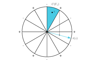
Our assumption on the separation margin is formally defined in Section C where we also give several examples and useful lemmas to bound γ\gamma. Our lower bounds in Section D are based on the following hard instance in 22 dimensions. The points are equally spaced and with alternating labels on the unit circle.

Formally, let nn be divisible by 44. We define the alternating points on the circle data set to be X={xk:=(cos(2kπn),sin(2kπn))k[n]}2X=\{x_{k}:=\left(\cos\left(\frac{2k\pi}{n}\right),\sin\left(\frac{2k\pi}{n}\right)\right)\mid k\in[n]\}\subset\mathbb{R}^{2}, and we put yk=(1)ky_{k}=(-1)^{k} for each k[n]k\in[n].

A natural choice for v¯\overline{v} would send any zdz\in\mathbb{R}^{d} to its closest point in our data set XX, multiplied by its label. However, applying Lemma C.2 gives us the following improved mapping, which is even optimal by Lemma C.5: note that for any zdz\in\mathbb{R}^{d} that is not collinear with any input point, there exists a unique izi_{z} such that zCone({xiz,xiz+1})z\in{\rm Cone}(\{x_{i_{z}},x_{i_{z}+1}\}). Instead of mapping to the closest input point, in what follows, we map to a point that is nearly orthogonal to zz,

rz:=xizyiz+xiz+1yiz+1xizxiz+12.\displaystyle r_{z}:=\frac{x_{i_{z}}y_{i_{z}}+x_{i_{z}+1}y_{i_{z}+1}}{\|x_{i_{z}}-x_{i_{z}+1}\|_{2}}.

More precisely we define v¯:dd\overline{v}:\mathbb{R}^{d}\rightarrow\mathbb{R}^{d} by

v¯(z)={0, if xiX,τ0:z=τxi(1)n/4+1rz, otherwise.\overline{v}(z)=\begin{cases}0&\text{, if }\exists x_{i}\in X,\tau\geq 0:z=\tau x_{i}\\ (-1)^{n/4+1}r_{z}&\text{, otherwise}.\end{cases}
Refer to caption
Figure 1: The picture shows how v¯(z)\overline{v}(z) is constructed: we subtract the vector x3x_{3} which is labeled 1-1 from the vector x2x_{2} which is labeled 11. We obtain rzr_{z} after rescaling to unit norm. Since n/4=3n/4=3 is odd we have v¯(z)=rz\overline{v}(z)=r_{z}.

See Fig. 1 for an illustration. We show in Lemma D.2 that γv¯=γ(X,Y)=Ω(n1)\gamma_{\overline{v}}=\gamma(X,Y)=\Omega(n^{-1}) and consequently n=Ω(γ1)n=\Omega(\gamma^{-1}). Now we can derive our lower bounds under increasingly stronger assumptions as follows:

For the first unconditional bound, Theorem 3.2, we map the input points on the unit circle by contraction to the unit 1\ell_{1} ball and note that by doing so, the labels remain in alternating order. Next we note that the output function ff of our network restricted to the 1\ell_{1} ball is a piecewise linear function of xx and thus its gradient fx\frac{\partial f}{\partial x} can only change in the vertices of the ball or where xx is orthogonal to one of the parameter vectors wsw_{s}, i.e., at most O(m)O(m) times. Now consider any triple of consecutive points. Since they have alternating labels, the gradient needs to change at least once for each triple. Consequently m=Ω(n)=Ω(γ1)m=\Omega(n)=\Omega(\gamma^{-1}), improving the Ω(γ1/2)\Omega(\gamma^{-1/2}) conditional lower bound in Ji and Telgarsky (2020). We remark that since the argument only depends on the output function but not on the loss function, Lemma D.4 yields an m=Ω(n)m=\Omega(n) lower bound for any loss function, in particular also for squared loss.

Now consider any argument that relies on an NTK analysis, where the fist step is to show that for our choice of the width mm, we have separability at initialization; this is how the argument in Ji and Telgarsky (2020) proceeds. Formally, assume that there exists Wm×dW\in\mathbb{R}^{m\times d} such that for all i[n]i\in[n], we have yifi(W0),W>0y_{i}\langle\nabla f_{i}(W_{0}),W\rangle>0. This condition enables us to show an improved lower bound, Theorem 3.3, as follows. Partition our data set into tuples, each consisting of four consecutive points. Now consider the event that there exists a point xix_{i} such that all parameter vectors wsw_{s} satisfy

𝟏[xi,ws>0]\displaystyle\mathbf{1}[\langle x_{i},w_{s}\rangle>0] =𝟏[xi+1,ws>0]=𝟏[xi+2,ws>0]=𝟏[xi+3,ws>0],\displaystyle=\mathbf{1}[\langle x_{i+1},w_{s}\rangle>0]=\mathbf{1}[\langle x_{i+2},w_{s}\rangle>0]=\mathbf{1}[\langle x_{i+3},w_{s}\rangle>0],

which implies that at least one of the points in {xi,xi+2,xi+3,xi+4}\{x_{i},x_{i+2},x_{i+3},x_{i+4}\} is misclassified. To avoid this, it means that our initialization necessarily needs to include, for each ii divisible by 44, a vector wsw_{s} that hits the areas orthogonal to the cones separating two points out of the quadruple. There are O(n)O(n) quadruples to hit, each succeeding with probability Ω(n1)\Omega(n^{-1}) with respect to the Gaussian measure. This is exactly the coupon collector’s problem, where the coupons are the quadruples, and it is known Erdős and Rényi (1961) that m=Ω(nlogn)=Ω(γ1logn)m=\Omega(n\log n)=\Omega(\gamma^{-1}\log n) are necessary to collect all O(n)O(n) items with constant probability, which yields our improved lower bound for this style of analysis. One thus needs a different approach beyond NTK to break this barrier, cf. Ji and Telgarsky (2020).

For the upper bound, Theorem 3.1, we further note that the existence of an NTK separator WW as above is not sufficient, i.e., we need to construct a separator U¯\overline{U} satisfying the separability condition. Moreover, to achieve a reasonable bound in terms of the margin parameter γ1\gamma^{-1} we also need that U¯\overline{U} achieves a separation margin of Ω(γ)\Omega(\gamma). To do so, it seems natural to construct U¯\overline{U} such that u¯j=ajv¯(wj)/m\overline{u}_{j}=a_{j}\overline{v}(w_{j})/\sqrt{m} for all j[m]j\in[m]. Indeed, this is the most natural choice because the resulting separation margin in the finite case is exactly the empirical mean estimator for the infinite case and thus standard concentration bounds (Hoeffing’s bound) yield the necessary proximity of the margins between the two cases, cf. Eq. (8). Let us assume we fix this choice of U¯\overline{U}. This condition enables us to prove a quadratic lower bound, Lemma 3.4, which shows that our analysis of the upper bound is actually tight: for our alternating points on a circle example, the summands have high variance, and therefore Hoeffding’s bound is tight by a matching lower bound Feller (1943). Consequently, m=Ω(γ2logn)m=\Omega(\gamma^{2}\log n), and one would need a different definition of U¯\overline{U} and a non-standard estimation of γ\gamma to break this barrier.

Finally, we conjecture that the quadratic upper bound is actually tight in general. Specifically, we conjecture the following: take n=1/γ2n=1/\gamma^{2} random points on the sphere in Θ(log(1/γ))\Theta(\log(1/\gamma)) dimensions and assign random labels yi{1,1}y_{i}\in\{-1,1\}. Then the NTK margin is Ω(γ)\Omega(\gamma).

If the conjecture is true, we obtain an Ω(1/γ2)\Omega(1/\gamma^{2}) lower bound for mm, up to logarithmic factors.777This might be confusing, since we argued before that such data is particularly mild for the squared loss function. This may be due to the different loss functions, but regardless, it does not contradict the O~(n/d)\widetilde{O}(n/d) bound of Daniely (2020) for the same data distribution in the squared loss regime, since n/d=Θ(1/(γ2log(1/γ)))n/d=\Theta(1/(\gamma^{2}\log(1/\gamma))). Indeed, we can round the weights to the nearest vectors in a net of size poly(1/γ)O(log(1/γ))\operatorname{poly}(1/\gamma)^{O(\log(1/\gamma))}, which only changes γ\gamma by a constant factor. Then, if we could classify with zero error, we would encode n=1/γ2n=1/\gamma^{2} random labels using mlogO(1)(1/γ)m\log^{O(1)}(1/\gamma) bits, which implies mΩ(1/(γ2logO(1)(1/γ)))m\geq\Omega(1/(\gamma^{2}\log^{O(1)}(1/\gamma))). We note that Ji and Telgarsky (2020) gave an O(1/n)O(1/\sqrt{n}) upper bound for the margin of any data with random labels, but we would need a matching Ω(1/n)\Omega(1/\sqrt{n}) lower bound for this instance in order for this argument to work.

4.3 Polynomial Width for Squared Loss

The high level intuition of our proof of Theorem 3.6 is to recursively prove the following: (1) the weight matrix does not change much, and (2) given that the weight matrix does not change much, the prediction error, measured by the squared loss, decays exponentially.

Given (1) we prove (2) as follows. The intuition is that the kernel matrix does not change much, since the weights do not change much, and it is close to the initial value of the kernel matrix, which is in turn close to the NTK matrix, involving the entire Gaussian distribution rather than our finite sample. The NTK matrix has a lower bound on its minimum eigenvalue by Assumption 3.3. Thus, the prediction loss decays exponentially.

Given (2) we prove (1) as follows. Since the prediction error decays exponentially, one can show that the change in weights is upper bounded by the prediction loss, and thus the change in weights also decays exponentially and the total change is small.

First, we show a concentration lemma for initialization:

Lemma 4.1 (Informal version of Lemma G.1).

Let m=m0Bm=m_{0}B. Let {w1,w2,,wm}d\{w_{1},w_{2},\ldots,w_{m}\}\subset\mathbb{R}^{d} denote a collection of vectors constructed as in Definition 2.1. We define Hcts,Hdisn×nH^{\operatorname{cts}},H^{\operatorname{dis}}\in\mathbb{R}^{n\times n} as follows

Hi,jcts:=𝔼w𝒩(0,I)[xixj𝟏wxi0,wxj0],Hi,jdis:=1mr=1m[xixj𝟏wrxi0,wrxj0].\displaystyle H^{\operatorname{cts}}_{i,j}:=\operatorname*{{\mathbb{E}}}_{w\sim\mathcal{N}(0,I)}\left[x_{i}^{\top}x_{j}{\bf 1}_{w^{\top}x_{i}\geq 0,w^{\top}x_{j}\geq 0}\right],\qquad H^{\operatorname{dis}}_{i,j}:=\frac{1}{m}\sum_{r=1}^{m}\left[x_{i}^{\top}x_{j}{\bf 1}_{w_{r}^{\top}x_{i}\geq 0,w_{r}^{\top}x_{j}\geq 0}\right].

Let λ=λmin(Hcts)\lambda=\lambda_{\min}(H^{\operatorname{cts}}). If m0=Ω(λ2n2log(nB/δ))m_{0}=\Omega(\lambda^{-2}n^{2}\log(nB/\delta)), we have that

HdisHctsFλ4,andλmin(Hdis)34λ\displaystyle\|H^{\operatorname{dis}}-H^{\operatorname{cts}}\|_{F}\leq\frac{\lambda}{4},\mathrm{~{}and~{}}\lambda_{\min}(H^{\operatorname{dis}})\geq\frac{3}{4}\lambda

holds with probability at least 1δ1-\delta.

Second, we can show a perturbation bound for random weights.

Lemma 4.2 (Informal version of Lemma G.2).

Let R(0,1)R\in(0,1). Let {w1,w2,,wm}\{w_{1},w_{2},\ldots,w_{m}\} denote a collection of weight vectors constructed as in Definition 2.1. For any set of weight vectors w~1,,w~md\widetilde{w}_{1},\ldots,\widetilde{w}_{m}\in\mathbb{R}^{d} that satisfy that for any r[m]r\in[m], w~rwr2R\|\widetilde{w}_{r}-w_{r}\|_{2}\leq R, consider the map H:m×dn×nH:\mathbb{R}^{m\times d}\rightarrow\mathbb{R}^{n\times n} defined by H(w)i,j:=1mxixjr=1m𝟏w~rxi0,w~rxj0H(w)_{i,j}:=\frac{1}{m}x_{i}^{\top}x_{j}\sum_{r=1}^{m}{\bf 1}_{\widetilde{w}_{r}^{\top}x_{i}\geq 0,\widetilde{w}_{r}^{\top}x_{j}\geq 0}. Then we have that H(w)H(w~)F<2nR\|H(w)-H(\widetilde{w})\|_{F}<2nR holds with probability at least 1n2Bexp(m0R/10)1-n^{2}\cdot B\cdot\exp(-m_{0}R/10).

Next, we have the following lemma (see Section I for a formal proof) stating that the weights should not change too much. Note that the lemma is a variation of Corollary 4.1 in Du et al. (2019c).

Lemma 4.3.

If Eq. (16) holds for i=0,,ki=0,\ldots,k, then we have for all r[m]r\in[m]

wr(t+1)wr(0)24nyu(0)2mλ:=D.\displaystyle\|w_{r}(t+1)-w_{r}(0)\|_{2}\leq\frac{4\sqrt{n}\|y-u(0)\|_{2}}{m\lambda}:=D.

Next, we calculate the difference of predictions between two consecutive iterations, analogous to the 𝖽ui(t)𝖽t\frac{\mathsf{d}u_{i}(t)}{\mathsf{d}t} term in Fact H.1. For each i[n]i\in[n], we have

ui(t+1)ui(t)=r=1m\displaystyle u_{i}(t+1)-u_{i}(t)=\sum_{r=1}^{m} ar(ϕ(wr(t+1)xi)ϕ(wr(t)xi))=r=1marzi,r.\displaystyle a_{r}\cdot\left(\phi(w_{r}(t+1)^{\top}x_{i})-\,\phi(w_{r}(t)^{\top}x_{i})\right)=\sum_{r=1}^{m}a_{r}\cdot z_{i,r}.

where

zi,r:=ϕ((wr(t)ηL(W(t))wr(t))xi)ϕ(wr(t)xi).\displaystyle z_{i,r}:=\phi\left(\Big{(}w_{r}(t)-\eta\frac{\partial L(W(t))}{\partial w_{r}(t)}\Big{)}^{\top}x_{i}\right)-\phi(w_{r}(t)^{\top}x_{i}).

Here we divide the right hand side into two parts. First, v1,iv_{1,i} represents the terms for which the pattern does not change, while v2,iv_{2,i} represents the terms for which the pattern may change. For each i[n]i\in[n], we define the set Si[m]S_{i}\subset[m] as

Si:={r[m]:wd\displaystyle S_{i}:=~{}\{r\in[m]:\forall w\in\mathbb{R}^{d} s.t. wwr(0)2R, and 𝟏wr(0)xi0=𝟏wxi0}.\displaystyle\text{ s.t. }\|w-w_{r}(0)\|_{2}\leq R,\text{ and }\mathbf{1}_{w_{r}(0)^{\top}x_{i}\geq 0}=\mathbf{1}_{w^{\top}x_{i}\geq 0}\}.

Then we define v1,iv_{1,i} and v2,iv_{2,i} as follows

v1,i:=rSiarzi,r,v2,i:=rS¯iarzi,r.\displaystyle v_{1,i}:=\sum_{r\in S_{i}}a_{r}z_{i,r},\qquad v_{2,i}:=\sum_{r\in\overline{S}_{i}}a_{r}z_{i,r}.

Define HH and Hn×nH^{\bot}\in\mathbb{R}^{n\times n} as

H(t)i,j:=\displaystyle H(t)_{i,j}:= 1mr=1mxixj𝟏wr(t)xi0,wr(t)xj0,\displaystyle~{}\frac{1}{m}\sum_{r=1}^{m}x_{i}^{\top}x_{j}{\bf 1}_{w_{r}(t)^{\top}x_{i}\geq 0,w_{r}(t)^{\top}x_{j}\geq 0}, (9)
H(t)i,j:=\displaystyle H(t)^{\bot}_{i,j}:= 1mrS¯ixixj𝟏wr(t)xi0,wr(t)xj0,\displaystyle~{}\frac{1}{m}\sum_{r\in\overline{S}_{i}}x_{i}^{\top}x_{j}{\bf 1}_{w_{r}(t)^{\top}x_{i}\geq 0,w_{r}(t)^{\top}x_{j}\geq 0}, (10)

and

C1:=2η(yu(t))H(t)(yu(t)),C2:=+2η(yu(t))H(t)(yu(t)),\displaystyle C_{1}:=-2\eta(y-u(t))^{\top}H(t)(y-u(t)),\qquad C_{2}:=+2\eta(y-u(t))^{\top}H(t)^{\bot}(y-u(t)),
C3:=2(yu(t))v2,C4:=u(t+1)u(t)22.\displaystyle C_{3}:=-2(y-u(t))^{\top}v_{2},\qquad\qquad\qquad\qquad\!C_{4}:=\|u(t+1)-u(t)\|_{2}^{2}.

Then we have that (see Section I for a formal proof)

Claim 4.4.

yu(t+1)22=yu(t)22+C1+C2+C3+C4.\|y-u(t+1)\|_{2}^{2}=\|y-u(t)\|_{2}^{2}+C_{1}+C_{2}+C_{3}+C_{4}.

Applying Claim I.2, I.3, I.4 and I.5 with the appropriate choice of parameters, we can show that the 2\ell_{2} norm shrinks in each iteration tt: yu(t+1)22yu(t)22α\|y-u(t+1)\|_{2}^{2}\leq\|y-u(t)\|_{2}^{2}\cdot\alpha, where α=(1mηλ+8mηnR+8mηnR+m2η2n2)\alpha=(1-m\eta\lambda+8m\eta nR+8m\eta nR+m^{2}\eta^{2}n^{2}).

5 Discussion

We present a novel worst case analysis using an initialization scheme for neural networks involving coupled weights. This technique is versatile and can be applied in many different settings. We give an improved analysis based on this technique to reduce the parameterization required to show the convergence of 22-layer neural networks with ReLU activations in the under-parameterized regime for the logistic loss to m=O(γ2logn)m=O(\gamma^{-2}\log n), which significantly improves the prior O(γ8logn)O(\gamma^{-8}\log n) bound. We further introduce a new unconditional lower bound of m=Ω(γ1)m=\Omega(\gamma^{-1}) as well as conditional bounds to narrow the gap in this regime. We also reduce the amount of over-parameterization required for the standard squared loss function to roughly m=O(λ2n2)m=O(\lambda^{-2}n^{2}), improving the prior O(λ4n4)O(\lambda^{-4}n^{4}) bound, and coming closer to the Ω(n)\Omega(n) lower bound. We believe this is a significant theoretical advance towards explaining the behavior of 22-layer neural networks in different settings. It is an intriguing open question to close the gaps between upper and lower bounds in both the under and over-parameterized settings. We note that the quadratic dependencies arise for several fundamental reasons in our analysis, and are already required to show a large minimum eigenvalue λ\lambda of our kernel matrix, or a large separation margin γ\gamma at initialization. In the latter case we have provided partial evidence of optimality by showing that our analysis has an m=Ω(γ2logn)m=\Omega(\gamma^{-2}\log n) lower bound, as well as a candidate hard instance for any possible algorithm. Another future direction is to extend our results to more than two layers, which may be possible by increasing mm by a poly(L)\operatorname{poly}(L) factor, where LL denotes the network depth Chen et al. (2019). We note that this also has not been done in earlier work Ji and Telgarsky (2020).

Acknowledgements

We thank the anonymous reviewers and Binghui Peng for their valuable comments. Alexander Munteanu and Simon Omlor were supported by the German Research Foundation (DFG), Collaborative Research Center SFB 876, project C4 and by the Dortmund Data Science Center (DoDSc). David Woodruff would like to thank NSF grant No. CCF-1815840, NIH grant 5401 HG 10798-2, ONR grant N00014-18-1-2562, and a Simons Investigator Award.

References

  • Allen-Zhu et al. (2019a) Zeyuan Allen-Zhu, Yuanzhi Li, and Yingyu Liang. Learning and generalization in overparameterized neural networks, going beyond two layers. In Advances in neural information processing systems, pages 6155–6166, 2019a.
  • Allen-Zhu et al. (2019b) Zeyuan Allen-Zhu, Yuanzhi Li, and Zhao Song. A convergence theory for deep learning via over-parameterization. In ICML, 2019b.
  • Allen-Zhu et al. (2019c) Zeyuan Allen-Zhu, Yuanzhi Li, and Zhao Song. On the convergence rate of training recurrent neural networks. In NeurIPS, 2019c.
  • Arora et al. (2019a) Sanjeev Arora, Simon S Du, Wei Hu, Zhiyuan Li, Ruslan Salakhutdinov, and Ruosong Wang. On exact computation with an infinitely wide neural net. In NeurIPS. arXiv preprint arXiv:1904.11955, 2019a.
  • Arora et al. (2019b) Sanjeev Arora, Simon S Du, Wei Hu, Zhiyuan Li, and Ruosong Wang. Fine-grained analysis of optimization and generalization for overparameterized two-layer neural networks. In ICML. arXiv preprint arXiv:1901.08584, 2019b.
  • Bakshi et al. (2019) Ainesh Bakshi, Rajesh Jayaram, and David P Woodruff. Learning two layer rectified neural networks in polynomial time. In Conference on Learning Theory (COLT), pages 195–268. PMLR, 2019.
  • Bernstein (1924) Sergei Bernstein. On a modification of chebyshev’s inequality and of the error formula of laplace. Ann. Sci. Inst. Sav. Ukraine, Sect. Math, 1(4):38–49, 1924.
  • Blum et al. (2020) Avrim Blum, John Hopcroft, and Ravi Kannan. Foundations of Data Science. Cambridge University Press, 2020.
  • Brand et al. (2021) Jan van den Brand, Binghui Peng, Zhao Song, and Omri Weinstein. Training (overparametrized) neural networks in near-linear time. In ITCS, 2021.
  • Bubeck et al. (2020) Sébastien Bubeck, Ronen Eldan, Yin Tat Lee, and Dan Mikulincer. Network size and size of the weights in memorization with two-layers neural networks. In NeurIPS, 2020.
  • Cao and Gu (2019a) Yuan Cao and Quanquan Gu. A generalization theory of gradient descent for learning over-parameterized deep relu networks. CoRR, abs/1902.01384, 2019a. URL http://arxiv.org/abs/1902.01384.
  • Cao and Gu (2019b) Yuan Cao and Quanquan Gu. Generalization bounds of stochastic gradient descent for wide and deep neural networks. In NeurIPS, pages 10835–10845, 2019b.
  • Chen and Xu (2020) Lin Chen and Sheng Xu. Deep neural tangent kernel and laplace kernel have the same rkhs. arXiv preprint arXiv:2009.10683, 2020.
  • Chen et al. (2020) Sitan Chen, Adam R. Klivans, and Raghu Meka. Learning deep relu networks is fixed-parameter tractable. arXiv preprint arXiv:2009.13512, 2020.
  • Chen et al. (2019) Zixiang Chen, Yuan Cao, Difan Zou, and Quanquan Gu. How much over-parameterization is sufficient to learn deep relu networks? CoRR, abs/1911.12360, 2019. URL http://arxiv.org/abs/1911.12360.
  • Chernoff (1952) Herman Chernoff. A measure of asymptotic efficiency for tests of a hypothesis based on the sum of observations. The Annals of Mathematical Statistics, pages 493–507, 1952.
  • Collobert et al. (2011) Ronan Collobert, Jason Weston, Léon Bottou, Michael Karlen, Koray Kavukcuoglu, and Pavel Kuksa. Natural language processing (almost) from scratch. Journal of machine learning research, 12(ARTICLE):2493–2537, 2011.
  • Daniely (2020) Amit Daniely. Neural networks learning and memorization with (almost) no over-parameterization. In Advances in Neural Information Processing Systems 33, (NeurIPS), 2020.
  • Devlin et al. (2018) Jacob Devlin, Ming-Wei Chang, Kenton Lee, and Kristina Toutanova. Bert: Pre-training of deep bidirectional transformers for language understanding. arXiv preprint arXiv:1810.04805, 2018.
  • Du et al. (2019a) Simon S Du, Kangcheng Hou, Barnabás Póczos, Ruslan Salakhutdinov, Ruosong Wang, and Keyulu Xu. Graph neural tangent kernel: Fusing graph neural networks with graph kernels. arXiv preprint arXiv:1905.13192, 2019a.
  • Du et al. (2019b) Simon S Du, Jason D Lee, Haochuan Li, Liwei Wang, and Xiyu Zhai. Gradient descent finds global minima of deep neural networks. In International Conference on Machine Learning (ICML). https://arxiv.org/pdf/1811.03804, 2019b.
  • Du et al. (2019c) Simon S Du, Xiyu Zhai, Barnabas Poczos, and Aarti Singh. Gradient descent provably optimizes over-parameterized neural networks. In ICLR. https://arxiv.org/pdf/1810.02054, 2019c.
  • Erdős and Rényi (1961) P. Erdős and A. Rényi. On a classical problem of probability theory. Magyar Tud. Akad. Mat. Kutató Int. Közl., 6:215–220, 1961.
  • Feller (1943) William Feller. Generalization of a probability limit theorem of cramér. Trans. Am. Math. Soc., 54:361–372, 1943.
  • Ge et al. (2018) Rong Ge, Jason D. Lee, and Tengyu Ma. Learning one-hidden-layer neural networks with landscape design. In ICLR, 2018.
  • He et al. (2016) Kaiming He, Xiangyu Zhang, Shaoqing Ren, and Jian Sun. Deep residual learning for image recognition. In Proceedings of the IEEE conference on computer vision and pattern recognition (CVPR), pages 770–778, 2016.
  • Hoeffding (1963) Wassily Hoeffding. Probability inequalities for sums of bounded random variables. Journal of the American Statistical Association, 58(301):13–30, 1963.
  • Huang and Yau (2020) Jiaoyang Huang and Horng-Tzer Yau. Dynamics of deep neural networks and neural tangent hierarchy. In International Conference on Machine Learning (ICML), pages 4542–4551. PMLR, 2020.
  • Jacot et al. (2018) Arthur Jacot, Franck Gabriel, and Clément Hongler. Neural tangent kernel: convergence and generalization in neural networks. In Proceedings of the 32nd International Conference on Neural Information Processing Systems (NeurIPS), pages 8580–8589, 2018.
  • Ji and Telgarsky (2020) Ziwei Ji and Matus Telgarsky. Polylogarithmic width suffices for gradient descent to achieve arbitrarily small test error with shallow relu networks. In ICLR, 2020.
  • Kawaguchi and Huang (2019) Kenji Kawaguchi and Jiaoyang Huang. Gradient descent finds global minima for generalizable deep neural networks of practical sizes. In 2019 57th Annual Allerton Conference on Communication, Control, and Computing (Allerton), pages 92–99. IEEE, 2019.
  • Krizhevsky et al. (2012) Alex Krizhevsky, Ilya Sutskever, and Geoffrey E Hinton. Imagenet classification with deep convolutional neural networks. Advances in neural information processing systems, 25:1097–1105, 2012.
  • LeCun et al. (1998) Yann LeCun, Léon Bottou, Yoshua Bengio, and Patrick Haffner. Gradient-based learning applied to document recognition. Proceedings of the IEEE, 86(11):2278–2324, 1998.
  • Lee et al. (2020) Jason D Lee, Ruoqi Shen, Zhao Song, Mengdi Wang, and Zheng Yu. Generalized leverage score sampling for neural networks. In NeurIPS, 2020.
  • Li et al. (2021) Xiaoxiao Li, Meirui Jiang, Xiaofei Zhang, Michael Kamp, and Qi Dou. Fedbn: Federated learning on non-iid features via local batch normalization. In International Conference on Learning Representations (ICLR). https://openreview.net/forum?id=6YEQUn0QICG, 2021.
  • Li and Liang (2018) Yuanzhi Li and Yingyu Liang. Learning overparameterized neural networks via stochastic gradient descent on structured data. In NeurIPS, 2018.
  • Li and Yuan (2017) Yuanzhi Li and Yang Yuan. Convergence analysis of two-layer neural networks with ReLU activation. In Advances in neural information processing systems (NIPS), pages 597–607, 2017.
  • Nitanda et al. (2019) Atsushi Nitanda, Geoffrey Chinot, and Taiji Suzuki. Gradient descent can learn less over-parameterized two-layer neural networks on classification problems. arXiv preprint arXiv:1905.09870, 2019.
  • Oymak and Soltanolkotabi (2020) Samet Oymak and Mahdi Soltanolkotabi. Toward moderate overparameterization: Global convergence guarantees for training shallow neural networks. IEEE Journal on Selected Areas in Information Theory, 1(1):84–105, 2020.
  • Silver et al. (2016) David Silver, Aja Huang, Chris J Maddison, Arthur Guez, Laurent Sifre, George Van Den Driessche, Julian Schrittwieser, Ioannis Antonoglou, Veda Panneershelvam, Marc Lanctot, et al. Mastering the game of go with deep neural networks and tree search. nature, 529(7587):484–489, 2016.
  • Silver et al. (2017) David Silver, Julian Schrittwieser, Karen Simonyan, Ioannis Antonoglou, Aja Huang, Arthur Guez, Thomas Hubert, Lucas Baker, Matthew Lai, Adrian Bolton, et al. Mastering the game of go without human knowledge. nature, 550(7676):354–359, 2017.
  • Song and Yang (2019) Zhao Song and Xin Yang. Quadratic suffices for over-parametrization via matrix chernoff bound. arXiv preprint arXiv:1906.03593, 2019.
  • Song et al. (2021) Zhao Song, Shuo Yang, and Ruizhe Zhang. Does preprocessing help training over-parameterized neural networks? Advances in Neural Information Processing Systems (NeurIPS), 34, 2021.
  • StEx (2011) StEx StEx. How can we sum up sin and cos series when the angles are in arithmetic progression? https://math.stackexchange.com/questions/17966/, 2011. Accessed: 2021-05-21.
  • Szegedy et al. (2015) Christian Szegedy, Wei Liu, Yangqing Jia, Pierre Sermanet, Scott Reed, Dragomir Anguelov, Dumitru Erhan, Vincent Vanhoucke, and Andrew Rabinovich. Going deeper with convolutions. In Proceedings of the IEEE conference on computer vision and pattern recognition, pages 1–9, 2015.
  • Tropp (2015) Joel A Tropp. An introduction to matrix concentration inequalities. Foundations and Trends® in Machine Learning, 8(1-2):1–230, 2015.
  • Zhang et al. (2021) Jiawei Zhang, Yushun Zhang, Mingyi Hong, Ruoyu Sun, and Zhi-Quan Luo. When expressivity meets trainability: Fewer than nn neurons can work. In Advances in Neural Information Processing Systems 34 (NeurIPS), pages 9167–9180, 2021.
  • Zhong et al. (2017a) Kai Zhong, Zhao Song, and Inderjit S. Dhillon. Learning non-overlapping convolutional neural networks with multiple kernels. arXiv preprint arXiv:1711.03440, 2017a.
  • Zhong et al. (2017b) Kai Zhong, Zhao Song, Prateek Jain, Peter L. Bartlett, and Inderjit S. Dhillon. Recovery guarantees for one-hidden-layer neural networks. In ICML, 2017b.
  • Zou and Gu (2019) Difan Zou and Quanquan Gu. An improved analysis of training over-parameterized deep neural networks. In NeurIPS, pages 2053–2062, 2019.

Appendix

Appendix A Probability Tools

In this section we introduce the probability tools that we use in our proofs. Lemma A.1, A.2 and A.3 concern tail bounds for random scalar variables. Lemma A.4 concerns the cumulative density function of the Gaussian distribution. Finally, Lemma A.5 concerns a concentration result for random matrices.

Lemma A.1 (Chernoff bound Chernoff (1952)).

Let X=i=1nXiX=\sum_{i=1}^{n}X_{i}, where Xi=1X_{i}=1 with probability pip_{i} and Xi=0X_{i}=0 with probability 1pi1-p_{i}, and all XiX_{i} are independent. Let μ=𝔼[X]=i=1npi\mu=\operatorname*{{\mathbb{E}}}[X]=\sum_{i=1}^{n}p_{i}. Then
1. Pr[X(1+δ)μ]exp(δ2μ/3)\Pr[X\geq(1+\delta)\mu]\leq\exp(-\delta^{2}\mu/3), δ>0\forall\delta>0 ;
2. Pr[X(1δ)μ]exp(δ2μ/2)\Pr[X\leq(1-\delta)\mu]\leq\exp(-\delta^{2}\mu/2), 0<δ<1\forall 0<\delta<1.

Lemma A.2 (Hoeffding bound Hoeffding (1963)).

Let X1,,XnX_{1},\cdots,X_{n} denote nn independent bounded variables in [ai,bi][a_{i},b_{i}]. Let X=i=1nXiX=\sum_{i=1}^{n}X_{i}. Then we have

Pr[|X𝔼[X]|t]2exp(2t2i=1n(biai)2).\displaystyle\Pr[|X-\operatorname*{{\mathbb{E}}}[X]|\geq t]\leq 2\exp\left(-\frac{2t^{2}}{\sum_{i=1}^{n}(b_{i}-a_{i})^{2}}\right).
Lemma A.3 (Bernstein’s inequality Bernstein (1924)).

Let X1,,XnX_{1},\cdots,X_{n} be independent zero-mean random variables. Suppose that |Xi|M|X_{i}|\leq M almost surely, for all ii. Then, for all positive tt,

Pr[i=1nXi>t]exp(t2/2j=1n𝔼[Xj2]+Mt/3).\displaystyle\Pr\left[\sum_{i=1}^{n}X_{i}>t\right]\leq\exp\left(-\frac{t^{2}/2}{\sum_{j=1}^{n}\operatorname*{{\mathbb{E}}}[X_{j}^{2}]+Mt/3}\right).
Lemma A.4 (Anti-concentration of the Gaussian distribution).

Let X𝒩(0,σ2)X\sim{\mathcal{N}}(0,\sigma^{2}), that is, the probability density function of XX is given by ϕ(x)=12πσ2ex22σ2\phi(x)=\frac{1}{\sqrt{2\pi\sigma^{2}}}e^{-\frac{x^{2}}{2\sigma^{2}}}. Then

Pr[|X|t](23tσ,45tσ).\displaystyle\Pr[|X|\leq t]\in\left(\frac{2}{3}\frac{t}{\sigma},\frac{4}{5}\frac{t}{\sigma}\right).
Lemma A.5 (Matrix Bernstein, Theorem 6.1.1 in Tropp (2015)).

Consider a finite sequence {X1,,Xm}n1×n2\{X_{1},\cdots,X_{m}\}\subset\mathbb{R}^{n_{1}\times n_{2}} of independent, random matrices with common dimension n1×n2n_{1}\times n_{2}. Assume that

𝔼[Xi]=0,i[m]andXiM,i[m].\displaystyle\operatorname*{{\mathbb{E}}}[X_{i}]=0,\forall i\in[m]~{}~{}~{}\mathrm{and}~{}~{}~{}\|X_{i}\|\leq M,\forall i\in[m].

Let Z=i=1mXiZ=\sum_{i=1}^{m}X_{i}. Let Var[Z]\mathrm{Var}[Z] be the matrix variance statistic of the sum:

Var[Z]=max{i=1m𝔼[XiXi],i=1m𝔼[XiXi]}.\displaystyle\mathrm{Var}[Z]=\max\left\{\Big{\|}\sum_{i=1}^{m}\operatorname*{{\mathbb{E}}}[X_{i}X_{i}^{\top}]\Big{\|},\Big{\|}\sum_{i=1}^{m}\operatorname*{{\mathbb{E}}}[X_{i}^{\top}X_{i}]\Big{\|}\right\}.

Then

𝔼[Z](2Var[Z]log(n1+n2))1/2+Mlog(n1+n2)/3.\displaystyle\operatorname*{{\mathbb{E}}}[\|Z\|]\leq(2\mathrm{Var}[Z]\cdot\log(n_{1}+n_{2}))^{1/2}+M\cdot\log(n_{1}+n_{2})/3.

Furthermore, for all t0t\geq 0,

Pr[Zt](n1+n2)exp(t2/2Var[Z]+Mt/3).\displaystyle\Pr[\|Z\|\geq t]\leq(n_{1}+n_{2})\cdot\exp\left(-\frac{t^{2}/2}{\mathrm{Var}[Z]+Mt/3}\right).
Lemma A.6 (Feller (1943)).

Let ZZ be a sum of independent random variables, each attaining values in [0,1][0,1], and let σ=𝐕𝐚𝐫(Z)200\sigma=\sqrt{\operatorname*{{\bf{Var}}}(Z)}\geq 200. Then for all t[0,σ2100]t\in[0,\frac{\sigma^{2}}{100}] we have

Pr[X𝔼[X]+t]cexp(t2/(3σ2))\Pr[X\geq\operatorname*{{\mathbb{E}}}[X]+t]\geq c\cdot\exp(-t^{2}/(3\sigma^{2}))

where c>0c>0 is some fixed constant.

Appendix B Preliminaries for log width under logistic loss

We consider a set of data points x1,,xndx_{1},\dots,x_{n}\in\mathbb{R}^{d} with xi2=1\|x_{i}\|_{2}=1 and labels y1,,yn{1,1}y_{1},\dots,y_{n}\in\{-1,1\}. The two layer network is parameterized by m,amm\in\mathbb{N},a\in\mathbb{R}^{m} and Wm×dW\in\mathbb{R}^{m\times d} as follows: we set the output function

f(x,W,a)=1ms=1masϕ(ws,x),\displaystyle f(x,W,a)=\frac{1}{\sqrt{m}}\sum_{s=1}^{m}a_{s}\phi\left(\langle w_{s},x\rangle\right),

which is scaled by a factor 1/m1/\sqrt{m} compared to the presentation in the main body to simplify notation, and to be more closely comparable to Ji and Telgarsky (2020). The changed initialization yields initial output of 0, independent of the normalization, and thus, consistent with the introduction, we could as well omit the normalization here and instead use it only in the learning rate. The main improvement of the network width comes from the fact that the learning rate is no compromise between the right normalization in the initial state and the appropriate progress in the gradient iterations, but can be adjusted to ensure the latter independent of the former. In the output function, ϕ(v)=max{0,v}\phi(v)=\max\{0,v\} denotes the ReLU function for vv\in\mathbb{R}. To simplify notation we set fi(W)=f(xi,W,a)f_{i}(W)=f(x_{i},W,a). Further we set (v)=ln(1+exp(v))\ell(v)=\ln(1+\exp(-v)) to be the logistic loss function. We use a random initialization W0,a0W_{0},a_{0} given in Definition 2.1. Our goal is to minimize the empirical loss of WW given by

R(W)=1ni=1n(yifi(W)).R(W)=\frac{1}{n}\sum_{i=1}^{n}\ell\left(y_{i}f_{i}(W)\right).

To accomplish this, we use a standard gradient descent algorithm. More precisely for t0t\geq 0 we set

Wt+1=WtηR(Wt)\displaystyle W_{t+1}=W_{t}-\eta\nabla R(W_{t})

for some step size η\eta. Further, it holds that

R(W)=1ni=1nyifi(W)(yifi(W)).\displaystyle\nabla R(W)=\frac{1}{n}\sum_{i=1}^{n}y_{i}\nabla f_{i}(W)\ell^{\prime}\left(y_{i}f_{i}(W)\right).

Moreover, we use the following notation

fi(t)(W):=fi(Wt),W\displaystyle f_{i}^{(t)}(W):=\langle\nabla f_{i}(W_{t}),W\rangle

and

R(t)(W):=i=1n(yifi(t)(W)).\displaystyle R^{(t)}(W):=\sum_{i=1}^{n}\ell\left(y_{i}f_{i}^{(t)}(W)\right).

Note that fi(W)ws=1mas𝟏[ws,xi>0]xi\frac{\partial f_{i}(W)}{\partial w_{s}}=\frac{1}{\sqrt{m}}a_{s}\mathbf{1}[\langle w_{s},x_{i}\rangle>0]x_{i}. In particular the gradient is independent of ws2\|w_{s}\|_{2}, which will be crucial in our improved analysis.

Appendix C Main assumption and examples

C.1 Main assumption

Here, we define the parameter γ>0\gamma>0 which was also used in Ji and Telgarsky (2020). Intuitively, γ\gamma determines the separation margin of the NTK. Let B=Bd={xd|x21}B=B^{d}=\{x\in\mathbb{R}^{d}~{}|~{}\|x\|_{2}\leq 1\} be the unit ball in dd dimensions. We set B\mathcal{F}_{B} to be the set of functions ff mapping from dom(f)=d{\rm dom}(f)=\mathbb{R}^{d} to range(f)=B{\rm range}(f)=B. Let μ𝒩\mu_{\mathcal{N}} denote the Gaussian measure on d\mathbb{R}^{d}, specified by the Gaussian density with respect to the Lebesgue measure on d\mathbb{R}^{d}.

Definition C.1.

Given a data set (X,Y)n×d×n(X,Y)\in\mathbb{R}^{n\times d}\times\mathbb{R}^{n} and a map v¯B\overline{v}\in\mathcal{F}_{B} we set

γv¯=γv¯(X,Y):=mini[n]yiv¯(z),xi𝟏[xi,z>0]𝖽μ𝒩(z).\displaystyle\gamma_{\overline{v}}=\gamma_{\overline{v}}(X,Y):=\min_{i\in[n]}y_{i}\int\langle\overline{v}(z),x_{i}\rangle\mathbf{1}[\langle x_{i},z\rangle>0]~{}\mathsf{d}\mu_{\mathcal{N}}(z).

We say that v¯\overline{v} is optimal if γv¯=γ(X,Y):=maxv¯Bγv¯\gamma_{\overline{v}}=\gamma(X,Y):=\max_{\overline{v}^{\prime}\in\mathcal{F}_{B}}\gamma_{\overline{v}^{\prime}}.

We note that maxv¯Bγv¯\max_{\overline{v}^{\prime}\in\mathcal{F}_{B}}\gamma_{\overline{v}^{\prime}} always exists since B\mathcal{F}_{B} is a set of bounded functions on a compact subset of d\mathbb{R}^{d}. We make the following assumption, which is also used in Ji and Telgarsky (2020):

Assumption C.1.

It holds that γ=γ(X,Y)>0\gamma=\gamma(X,Y)>0.

Before we prove our main results we show some properties of v¯\overline{v} to develop a better understanding of our assumption. The following lemma shows that the integral can be viewed as a finite sum over certain cones in d\mathbb{R}^{d}. Given U{1,2,,n}=[n]U\subseteq\{1,2,\dots,n\}=[n] we define the cone

C(U):={xd|x,xi>0 if and only if iU}.\displaystyle C(U):=\{x\in\mathbb{R}^{d}~{}|~{}\langle x,x_{i}\rangle>0\text{ if and only if $i\in U$}\}.

Note that C()={xd|x,xi0 for all i[n]}C(\emptyset)=\{x\in\mathbb{R}^{d}~{}|~{}\langle x,x_{i}\rangle\leq 0\text{ for all $i\in[n]$}\} and that d=˙U[n]C(U)\mathbb{R}^{d}=\dot{\bigcup}_{U\subseteq[n]}C(U). Further we set P(U)P(U) to be the probability that a random Gaussian is an element of C(U)C(U) and PUP_{U} to be the probability measure of random Gaussians z𝒩(0,I)z\sim\mathcal{N}(0,I) restricted to the event that zC(U)z\in C(U). The following lemma shows that we do not have to consider each mapping in B\mathcal{F}_{B} but it suffices to focus on a specific subset. More precisely we can assume that v¯\overline{v} is constant on the cones C(U)C(U). In particular this means we can assume v¯(z)=v¯(cz)\overline{v}(z)=\overline{v}(cz) for any zdz\in\mathbb{R}^{d} and scalar c>0c>0 and that v¯\overline{v} is locally constant.

Lemma C.2.

Let v¯B\overline{v}\in\mathcal{F}_{B}. Then there exists v¯\overline{v}^{\prime} such that γv¯=γv¯\gamma_{\overline{v}^{\prime}}=\gamma_{\overline{v}} and v¯\overline{v}^{\prime} is constant on C(U)C(U) for any U[n]U\subseteq[n].

Proof.

Observe that for any distinct U,U[n]U,U^{\prime}\subseteq[n] the cones C(U)C(U) and C(U)C(U^{\prime}) are disjoint since for any xdx\in\mathbb{R}^{d} the cone C(Ux)C(U_{x}) containing xx is given by Ux={i[n]|x,xi>0}U_{x}=\{i\in[n]~{}|~{}\langle x,x_{i}\rangle>0\}. Further we have that U[n]C(U)=d\bigcup_{U\subseteq[n]}C(U)=\mathbb{R}^{d} since any xdx\in\mathbb{R}^{d} is included in some C(Ux)C(U_{x}). Thus for any i[n]i\in[n] we have

yiv¯(z),xi𝟏[xi,z>0]𝖽μ𝒩(z)\displaystyle y_{i}\int\langle\overline{v}(z),x_{i}\rangle\mathbf{1}[\langle x_{i},z\rangle>0]~{}\mathsf{d}\mu_{\mathcal{N}}(z) =yiU[n]P(U)v¯(z),xi𝟏[xi,z>0]𝖽PU(z)\displaystyle=y_{i}\sum_{U\subseteq[n]}P(U)\int\langle\overline{v}(z),x_{i}\rangle\mathbf{1}[\langle x_{i},z\rangle>0]~{}\mathsf{d}P_{U}(z)
=yiU[n],iUP(U)v¯(z),xi𝖽PU(z)\displaystyle=y_{i}\sum_{U\subseteq[n],i\in U}P(U)\int\langle\overline{v}(z),x_{i}\rangle~{}\mathsf{d}P_{U}(z)
=yiU[n],iUP(U)xi,v¯(z)𝖽PU(z).\displaystyle=y_{i}\sum_{U\subseteq[n],i\in U}P(U)~{}\langle x_{i},\int\overline{v}(z)~{}\mathsf{d}P_{U}(z)\rangle.

Hence defining v¯(x)=P(Ux)v¯(z)𝖽PUx(z)\overline{v}^{\prime}(x)=P(U_{x})\int\overline{v}(z)~{}\mathsf{d}P_{U_{x}}(z) satisfies

yiv¯(z),xi𝟏[xi,z>0]𝖽μ𝒩(z)=yiv¯(z),xi𝟏[xi,z>0]𝖽μ𝒩(z)\displaystyle y_{i}\int\langle\overline{v}(z),x_{i}\rangle\mathbf{1}[\langle x_{i},z\rangle>0]~{}\mathsf{d}\mu_{\mathcal{N}}(z)=y_{i}\int\langle\overline{v}^{\prime}(z),x_{i}\rangle\mathbf{1}[\langle x_{i},z\rangle>0]~{}\mathsf{d}\mu_{\mathcal{N}}(z)

and since v¯(z)21\|\overline{v}(z)\|_{2}\leq 1 it follows that v¯(z)21\|\overline{v}^{\prime}(z)\|_{2}\leq 1 for all zdz\in\mathbb{R}^{d}. ∎

Next we give an idea how the dimension dd can impact γ\gamma. We show that in the simple case, where d\mathbb{R}^{d} can be divided into orthogonal subspaces, such that each data point xix_{i} is an element of one of the subspaces, there is a helpful connection between a mapping v¯B\overline{v}\in\mathcal{F}_{B} and the mapping that v¯\overline{v} induces on the subspaces.

Lemma C.3.

Assume there exist orthogonal subspaces V1,VsV_{1},\dots V_{s} of d\mathbb{R}^{d} with d=jsVj\mathbb{R}^{d}=\bigoplus_{j\leq s}V_{j} such that for each i[n]i\in[n] there exists j[s]j\in[s] such that xiVjx_{i}\in V_{j}. Then the following two statements hold:

Part 1. Assume that for each j[s]j\in[s] there exists γj>0\gamma_{j}>0 and v¯jB\overline{v}_{j}\in\mathcal{F}_{B} such that for all xiVjx_{i}\in V_{j} we have

yiv¯j(z),xi𝟏[xi,z>0]𝖽μ𝒩(z)γj.\displaystyle y_{i}\int\langle\overline{v}_{j}(z),x_{i}\rangle\mathbf{1}[\langle x_{i},z\rangle>0]~{}\mathsf{d}\mu_{\mathcal{N}}(z)\geq\gamma_{j}.

Then for each ρs\rho\in\mathbb{R}^{s} with ρ2=1\|\rho\|_{2}=1 there exists v¯B\overline{v}\in\mathcal{F}_{B} with

mini[n]yiv¯(z),xi𝟏[xi,z>0]𝖽μ𝒩(z)minj[s]ρjγj.\displaystyle\min_{i\in[n]}y_{i}\int\langle\overline{v}(z),x_{i}\rangle\mathbf{1}[\langle x_{i},z\rangle>0]~{}\mathsf{d}\mu_{\mathcal{N}}(z)\geq\min_{j\in[s]}\rho_{j}\gamma_{j}.

Part 2. Assume that v¯\overline{v} maximizes the term

γ=mini[n]yiv¯(z),xi𝟏[xi,z>0]𝖽μ𝒩(z),\gamma^{*}=\min_{i\in[n]}y_{i}\int\langle\overline{v}(z),x_{i}\rangle\mathbf{1}[\langle x_{i},z\rangle>0]~{}\mathsf{d}\mu_{\mathcal{N}}(z),

and that γ>0\gamma^{*}>0. Given any vector zdz\in\mathbb{R}^{d} we denote by pj(z)Vjp_{j}(z)\in V_{j} the projection of zz onto VjV_{j}. Let ρj=maxzdpj(v¯(z))2\rho_{j}^{\prime}=\max_{z\in\mathbb{R}^{d}}\|p_{j}(\overline{v}(z))\|_{2}. Then for all j[s]j\in[s] the mapping v¯j(z)=pj(v¯(z))ρj\overline{v}_{j}(z)=\frac{p_{j}(\overline{v}(z))}{\rho_{j}^{\prime}} maximizes

γj=minxiVjyiv¯j(z),xi𝟏[xi,z>0]𝖽μ𝒩(z)\gamma_{j}=\min_{x_{i}\in V_{j}}y_{i}\int\langle\overline{v}_{j}(z),x_{i}\rangle\mathbf{1}[\langle x_{i},z\rangle>0]~{}\mathsf{d}\mu_{\mathcal{N}}(z)

and it holds that v¯j(z)21\|\overline{v}_{j}(z)\|_{2}\leq 1 for all zdz\in\mathbb{R}^{d}. In other words if v¯\overline{v} is optimal for (X,Y)(X,Y) then v¯j\overline{v}_{j} is optimal for (Xj,Yj)(X_{j},Y_{j}) where Xj={xiVj|i[n]}X_{j}=\{x_{i}\in V_{j}~{}|~{}i\in[n]\} with the corresponding labels, i.e., yxi=yiy_{x_{i}}=y_{i}.

Proof.

Part 1.

Since applying the projection pjp_{j} onto VjV_{j} to any point zdz\in\mathbb{R}^{d} does not change the scalar product of zz and xiVjx_{i}\in V_{j}, i.e., xi,z=xi,pj(z)\langle x_{i},z\rangle=\langle x_{i},p_{j}(z)\rangle, we can assume that for all zdz\in\mathbb{R}^{d} we have v¯j(z)Vj\overline{v}_{j}(z)\in V_{j}. Let zdz\in\mathbb{R}^{d}. We define v¯(z):=j=1sρjv¯j(z)\overline{v}(z):=\sum_{j=1}^{s}\rho_{j}\overline{v}_{j}(z). Then by orthogonality

v¯(z)22=j=1sρj2v¯j(z)22j=1sρj21=1.\displaystyle\|\overline{v}(z)\|_{2}^{2}=\sum_{j=1}^{s}\rho_{j}^{2}\|\overline{v}_{j}(z)\|_{2}^{2}\leq\sum_{j=1}^{s}\rho_{j}^{2}\cdot 1=1.

Thus it holds that v¯B\overline{v}\in\mathcal{F}_{B}. Further we have xi,v¯(z)=k=1sρkxi,v¯k(z)=ρjxi,v¯j(z)\langle x_{i},\overline{v}(z)\rangle=\sum_{k=1}^{s}\rho_{k}\langle x_{i},\overline{v}_{k}(z)\rangle=\rho_{j}\langle x_{i},\overline{v}_{j}(z)\rangle for xiVjx_{i}\in V_{j} again by orthogonality it holds that

yiv¯(z),xi𝟏[xi,z>0]𝖽μ𝒩(z)=\displaystyle y_{i}\int\langle\overline{v}(z),x_{i}\rangle\mathbf{1}[\langle x_{i},z\rangle>0]~{}\mathsf{d}\mu_{\mathcal{N}}(z)= ρjyiv¯j(z),xi𝟏[xi,z>0]𝖽μ𝒩(z)ρjγj.\displaystyle~{}\rho_{j}y_{i}\int\langle\overline{v}_{j}(z),x_{i}\rangle\mathbf{1}[\langle x_{i},z\rangle>0]~{}\mathsf{d}\mu_{\mathcal{N}}(z)\geq~{}\rho_{j}\gamma_{j}.

Part 2.

For the sake of contradiction assume that there are ksk\leq s and v¯kB\overline{v}^{*}_{k}\in\mathcal{F}_{B} such that

γk=minxiVkyiv¯k(z),xi𝟏[xi,z>0]𝖽μ𝒩(z)=γk+ϵ\gamma^{*}_{k}=\min_{x_{i}\in V_{k}}y_{i}\int\langle\overline{v}_{k}(z),x_{i}\rangle\mathbf{1}[\langle x_{i},z\rangle>0]~{}\mathsf{d}\mu_{\mathcal{N}}(z)=\gamma_{k}+\epsilon

for some ϵ>0\epsilon>0. Using Part 1. we can construct a new mapping v¯B\overline{v}^{\prime}\in\mathcal{F}_{B} by using the mappings v¯j\overline{v}_{j} defined in the lemma for jkj\neq k, and exchange v¯k\overline{v}_{k} by v¯k\overline{v}_{k}^{*}. Also as in Part 1 let ρj=ρj+ϵ\rho_{j}=\rho_{j}^{\prime}+\epsilon^{\prime} for jkj\neq k and ρk=ρk2sϵρk\rho_{k}=\rho_{k}^{\prime}-2\frac{s\epsilon^{\prime}}{\rho_{k}^{\prime}} with ϵ=min{ρk24s,ρk2ϵ4(γk+ϵ)s}\epsilon^{\prime}=\min\{\frac{\rho_{k}^{\prime 2}}{4s},\frac{\rho_{k}^{\prime 2}\epsilon}{4(\gamma_{k}+\epsilon)s}\}. Then we have

2s+sϵ+4s2ϵρk24s.\displaystyle 2s+s\epsilon^{\prime}+4s^{2}\frac{\epsilon^{\prime}}{\rho_{k}^{\prime 2}}\leq 4s.

Subtracting 4s4s and multiplying with ϵ\epsilon^{\prime} gives us

2sϵ+sϵ24sϵ+4(sϵρk)20.\displaystyle 2s\epsilon^{\prime}+s\epsilon^{\prime 2}-4s\epsilon^{\prime}+4\left(\frac{s\epsilon^{\prime}}{\rho_{k}^{\prime}}\right)^{2}\leq 0.

Hence it holds that

j=1sρj2\displaystyle\sum_{j=1}^{s}\rho_{j}^{2}\leq (jk(ρj2+2ϵ+ϵ2))+ρk24sϵ+4(sϵρk)2\displaystyle~{}\left(\sum_{j\neq k}(\rho_{j}^{\prime 2}+2\epsilon^{\prime}+\epsilon^{\prime 2})\right)+\rho_{k}^{\prime 2}-{4s\epsilon^{\prime}}+4\left(\frac{s\epsilon^{\prime}}{\rho_{k}^{\prime}}\right)^{2}
\displaystyle\leq (j=1sρj2)+2sϵ+sϵ24sϵ+4(sϵρk)2j=1sρj21.\displaystyle~{}\left(\sum_{j=1}^{s}\rho_{j}^{\prime 2}\right)+2s\epsilon^{\prime}+s\epsilon^{\prime 2}-4s\epsilon^{\prime}+4\left(\frac{s\epsilon^{\prime}}{\rho_{k}^{\prime}}\right)^{2}\leq~{}\sum_{j=1}^{s}\rho_{j}^{\prime 2}\leq~{}1.

For any xiVjx_{i}\in V_{j} with jkj\neq k we have by orthogonality as in Part 1.

yiv¯(z),xi𝟏[xi,z>0]𝖽μ𝒩(z)\displaystyle y_{i}\int\langle\overline{v}^{\prime}(z),x_{i}\rangle\mathbf{1}[\langle x_{i},z\rangle>0]~{}\mathsf{d}\mu_{\mathcal{N}}(z) =ρjyiv¯j(z),xi𝟏[xi,z>0]𝖽μ𝒩(z)\displaystyle=\rho_{j}y_{i}\int\langle\overline{v}_{j}(z),x_{i}\rangle\mathbf{1}[\langle x_{i},z\rangle>0]~{}\mathsf{d}\mu_{\mathcal{N}}(z)
=(ρj+ϵ)yiv¯j(z),xi𝟏[xi,z>0]𝖽μ𝒩(z).\displaystyle=(\rho_{j}^{\prime}+\epsilon^{\prime})y_{i}\int\langle\overline{v}_{j}(z),x_{i}\rangle\mathbf{1}[\langle x_{i},z\rangle>0]~{}\mathsf{d}\mu_{\mathcal{N}}(z).

Further we have

minxiVkyiv¯(z),xi𝟏[xi,z>0]𝖽μ𝒩(z)=\displaystyle\min_{x_{i}\in V_{k}}y_{i}\int\langle\overline{v}^{\prime}(z),x_{i}\rangle\mathbf{1}[\langle x_{i},z\rangle>0]~{}\mathsf{d}\mu_{\mathcal{N}}(z)= ρkγk\displaystyle~{}\rho_{k}\gamma^{*}_{k}
=\displaystyle= (ρk2sρkϵ)(γk+ϵ)\displaystyle~{}(\rho_{k}^{\prime}-2\frac{s}{\rho_{k}}\epsilon^{\prime})(\gamma_{k}+\epsilon)
\displaystyle\geq ρkγk2sρkρk2ϵ4(γk+ϵ)s(γk+ϵ)+ρkϵ\displaystyle~{}\rho_{k}^{\prime}\gamma_{k}-\frac{2s}{\rho_{k}^{\prime}}\cdot\frac{\rho_{k}^{\prime 2}\epsilon}{4(\gamma_{k}+\epsilon)s}(\gamma_{k}+\epsilon)+\rho_{k}^{\prime}\epsilon
=\displaystyle= ρkγk+ρkϵ2.\displaystyle~{}\rho_{k}^{\prime}\gamma_{k}+\frac{\rho_{k}^{\prime}\epsilon}{2}.

We conclude again by orthogonality that

yiv¯(z),xi𝟏[xi,z>0]𝖽μ𝒩(z)=\displaystyle y_{i}\int\langle\overline{v}^{\prime}(z),x_{i}\rangle\mathbf{1}[\langle x_{i},z\rangle>0]~{}\mathsf{d}\mu_{\mathcal{N}}(z)= ρjyiv¯j(z),xi𝟏[xi,z>0]𝖽μ𝒩(z)\displaystyle~{}\rho_{j}y_{i}\int\langle\overline{v}^{\prime}_{j}(z),x_{i}\rangle\mathbf{1}[\langle x_{i},z\rangle>0]~{}\mathsf{d}\mu_{\mathcal{N}}(z)
>\displaystyle> minjρjγj\displaystyle~{}\min_{j}\rho_{j}^{\prime}\gamma_{j}
=\displaystyle= γ\displaystyle~{}\gamma^{*}

and thus v¯\overline{v}^{\prime} contradicts the maximizing choice of v¯\overline{v}. ∎

As a direct consequence we get that the problem of finding an optimal v¯\overline{v} for the whole data set can be reduced to finding an optimal v¯j\overline{v}_{j} for each subspace.

Corollary C.4.

Assume there exist orthogonal subspaces V1,VsV_{1},\dots V_{s} of d\mathbb{R}^{d} with d=jsVj\mathbb{R}^{d}=\bigoplus_{j\leq s}V_{j} such that for each i[n]i\in[n] there exists j[s]j\in[s] with xiVjx_{i}\in V_{j}. For j[s]j\in[s] let (Xj,Yj)(X_{j},Y_{j}) denote the data set consisting of all data points (xi,yi)(x_{i},y_{i}) where xiVjx_{i}\in V_{j}. Then v¯\overline{v} is optimal for (X,Y)(X,Y) if and only if for all j[s]j\in[s] the mapping v¯j\overline{v}_{j} defined in Lemma C.3 is optimal for (Xj,Yj)(X_{j},Y_{j}) and γv¯=j[s]γjρj\gamma_{\overline{v}}=\sum_{j\in[s]}\gamma_{j}\rho^{*}_{j} where ρ=argmaxρ𝒮s1minj[s]ρjγj\rho^{*}={\rm argmax}_{\rho\in\mathcal{S}^{s-1}}\min_{j\in[s]}\rho_{j}\gamma_{j}.

Proof.

One direction follows immediately by Lemma C.3 2) the other direction is a direct consequence of the formula given in Lemma C.3 1). ∎

The following bound for γ\gamma simplifies calculations in some cases of interest. It also gives us a natural candidate for an optimal v¯B\overline{v}\in\mathcal{F}_{B}. Given an instance (X,Y)(X,Y) recall that Uz={i[n]z,xi>0}U_{z}=\{i\in[n]\mid\langle z,x_{i}\rangle>0\}. We set

v¯0(z)=i[n]Uzxiyii[n]Uzxiyi2.\displaystyle\overline{v}_{0}(z)=\frac{\sum_{i\in[n]\cap U_{z}}x_{i}y_{i}}{\|\sum_{i\in[n]\cap U_{z}}x_{i}y_{i}\|_{2}}. (11)

We note that v¯0(z)\overline{v}_{0}(z) is not optimal in general but if instances have certain symmetry properties, then v¯0(z)\overline{v}_{0}(z) is optimal.

Lemma C.5.

For any subset S[n]S\subseteq[n] it holds that

γU[n]P(U)1|S|iSUxiyi2\displaystyle\gamma\leq\sum_{U\subseteq[n]}P(U)\frac{1}{|S|}\left\|\sum_{i\in S\cap U}x_{i}y_{i}\right\|_{2}
Proof.

By Lemma C.2 there exists an optimal v¯\overline{v} that is constant on C(U)C(U) for all U[n]U\subseteq[n]. For xUx\in U let zU=v¯(x)z_{U}=\overline{v}(x). Then by using an averaging argument and the Cauchy–Schwarz inequality we get

γ\displaystyle\gamma 1|S|iSyiv¯(z),xi𝟏[xi,z>0]𝖽μ𝒩(z)\displaystyle\leq\frac{1}{|S|}\sum_{i\in S}y_{i}\int\langle\overline{v}(z),x_{i}\rangle\mathbf{1}[\langle x_{i},z\rangle>0]~{}\mathsf{d}\mu_{\mathcal{N}}(z)
=1|S|iSyiU[n],iUP(U)xi,zU\displaystyle=\frac{1}{|S|}\sum_{i\in S}y_{i}\sum_{U\subseteq[n],i\in U}P(U)\langle x_{i},z_{U}\rangle
=1|S|U[n]P(U)iSUyixi,zU\displaystyle=\frac{1}{|S|}\sum_{U\subseteq[n]}P(U)\langle\sum_{i\in S\cap U}y_{i}x_{i},z_{U}\rangle
U[n]P(U)1|S|iSUxiyi2.\displaystyle\leq\sum_{U\subseteq[n]}P(U)\frac{1}{|S|}\left\|\sum_{i\in S\cap U}x_{i}y_{i}\right\|_{2}.

Finally we give an idea of how two points and their distance impacts the cones and their hitting probabilities.

Lemma C.6.

Let x1,x2𝒮d1x_{1},x_{2}\in\mathcal{S}^{d-1} be two points with x1,x2>0\langle x_{1},x_{2}\rangle>0 and x1x22=b>0\|x_{1}-x_{2}\|_{2}=b>0. Set V1={xd|x1,x>0x2,x}V_{1}^{\prime}=\{x\in\mathbb{R}^{d}~{}|~{}\langle x_{1},x\rangle>0\geq\langle x_{2},x\rangle\}. Then for a random Gaussian zz we have zV1z\in V_{1}^{\prime} with probability P(V1)P(V_{1}^{\prime}) where b7P(V1)b5\frac{b}{7}\leq P(V_{1}^{\prime})\leq\frac{b}{5}. Further for any zz with z2=1\|z\|_{2}=1 it holds that |x1,zx2,z|b|\langle x_{1},z\rangle-\langle x_{2},z\rangle|\leq b.

Proof.

We define V1={x|x1,x>0}V_{1}=\{x\in\mathbb{R}~{}|~{}\langle x_{1},x\rangle>0\}. Then P(V1)=12P(V_{1})=\frac{1}{2} since for a random Gaussian zz it holds that x1,z>0\langle x_{1},z\rangle>0 with probability 12\frac{1}{2}. Since the space spanned by x1x_{1} and x2x_{2} is 22-dimensional, we can assume that x1x_{1} and x2x_{2} are on the unit circle and that x1=(1,0)x_{1}=(1,0) and x2=(cos(φ),sin(φ))x_{2}=(\cos(\varphi),\sin(\varphi)) for φπ2\varphi\leq\frac{\pi}{2}. Note that P(V1)P(V_{1}^{\prime}) is given by b2π\frac{b^{\prime}}{2\pi} where b=φb^{\prime}=\varphi is the length of the arc connecting x1x_{1} and x2x_{2} on the circle. Since bb is the Euclidean distance and thus the shortest distance between x1x_{1} and x2x_{2} we have bbb\leq b^{\prime}. Further it holds that

h(φ):=bb=φ(1cos(φ))2+sin(φ)2=φ22cos(φ).h(\varphi):=\frac{b^{\prime}}{b}=\frac{\varphi}{\sqrt{(1-\cos(\varphi))^{2}+\sin(\varphi)^{2}}}=\frac{\varphi}{\sqrt{2-2\cos(\varphi)}}.

Then h(φ)h^{\prime}(\varphi) is positive on (0,π2](0,\frac{\pi}{2}], so h(φ)h(\varphi) is monotonously non-decreasing, and thus h(φ)h(π2)=(π/2)2=π8h(\varphi)\leq h(\frac{\pi}{2})=\frac{(\pi/2)}{\sqrt{2}}=\frac{\pi}{\sqrt{8}} and bbπ8b^{\prime}\leq b\cdot\frac{\pi}{\sqrt{8}}. Consequently for P(V1)=b2πP(V_{1}^{\prime})=\frac{b^{\prime}}{2\pi} we have that

b7b2πP(V1)b2ππ8b5.\displaystyle\frac{b}{7}\leq\frac{b}{2\pi}\leq P(V_{1}^{\prime})\leq\frac{b}{2\pi}\cdot\frac{\pi}{\sqrt{8}}\leq\frac{b}{5}.

For the second part we note that for any zz with z2=1\|z\|_{2}=1 we get

|z,x1z,x2|=|z,x1x2|z2x1x22=1b\displaystyle|\langle z,x_{1}\rangle-\langle z,x_{2}\rangle|=|\langle z,x_{1}-x_{2}\rangle|\leq\|z\|_{2}\|x_{1}-x_{2}\|_{2}=1\cdot b

by using the Cauchy–Schwarz inequality. ∎

C.2 Example 1: Orthogonal unit vectors

Let us start with a simple example first: let eide_{i}\in\mathbb{R}^{d} be the ii-th unit vector. Let n=2dn=2d, xi=eix_{i}=e_{i} for idi\leq d and xi=eidx_{i}=-e_{i-d} otherwise with arbitrary labels. First consider the instance (Xi,Yi)(X_{i},Y_{i}) created by the points xix_{i} and xi+dx_{i+d} for idi\leq d. Then we note that v¯i\overline{v}_{i} sending any point zz with z,ei>0\langle z,e_{i}\rangle>0 to eiyie_{i}y_{i} and any other point to eiyi+d-e_{i}y_{i+d} is optimal since it holds that γi=γv¯i(Xi,Yi)=1𝟏[xi,z>0]𝖽μ𝒩(z)=12\gamma_{i}=\gamma_{\overline{v}_{i}}(X_{i},Y_{i})=\int 1\cdot\mathbf{1}[\langle x_{i},z\rangle>0]~{}\mathsf{d}\mu_{\mathcal{N}}(z)=\frac{1}{2}. Since the subspaces Vi=span{ei}V_{i}=\operatorname{span}\{e_{i}\} are orthogonal we can apply Corollary C.4 with vector ρ=(1d)d\rho=(\frac{1}{\sqrt{d}})^{d}. Thus the optimal γ\gamma for our instance is 12d\frac{1}{2\sqrt{d}}.

C.3 Example 2: Two differently labeled points at distance bb

Refer to caption
Figure 2: a) Two points x1x_{1} and x2x_{2} on the sphere. C(U)C(U) is the cone consisting of vectors having positive scalar product with both points. The cone C(Ui)C(U_{i}) consists of vectors having positive scalar product with xix_{i} but negative scalar product with the other point. b) The probability P(Ui)P(U_{i}) of a random Gaussian being in the cone C(Ui)C(U_{i}) is exactly the length of the shortest arc on the circle (which is close to the Euclidean distance) connecting the points, divided by 2π2\pi.

The next example is a set of two points x1,x2dx_{1},x_{2}\in\mathbb{R}^{d} with y1=1=y2y_{1}=1=-y_{2} and x1,x2>0\langle x_{1},x_{2}\rangle>0. Let U1={1},U2={2},U={1,2}U_{1}=\{1\},U_{2}=\{2\},U=\{1,2\} and V1={x|x1,x>0}V_{1}=\{x\in\mathbb{R}~{}|~{}\langle x_{1},x\rangle>0\}. Then P(U)=P(V1)P(U1)12b5P(U)=P(V_{1})-P(U_{1})\geq\frac{1}{2}-\frac{b}{5} by Lemma C.6 and P(U1)=P(U2)=P(V1)P(U)12(12b5)=b5P(U_{1})=P(U_{2})=P(V_{1})-P(U)\leq\frac{1}{2}-(\frac{1}{2}-\frac{b}{5})=\frac{b}{5}. For an illustration see Figure 2.

By Lemma C.2 we can assume that there exists an optimal v¯\overline{v} which is constant on C(U)C(U) and constant on C(Ui)C(U_{i}) for i{1,2}i\in\{1,2\}, i.e., that v¯(z)=zB\overline{v}(z)=z^{\prime}\in B for all zC(U)z\in C(U) and v¯(z)=z′′B\overline{v}(z)=z^{\prime\prime}\in B for all zC(U1)z\in C(U_{1}).

By Lemma C.6 we have |x1,zx2,z|b|\langle x_{1},z^{\prime}\rangle-\langle x_{2},z^{\prime}\rangle|\leq b. Consequently since x1x_{1} and x2x_{2} have different labels there exists at least one i{1,2}i\in\{1,2\} with z,xiyib/2\langle z^{\prime},x_{i}\rangle y_{i}\leq b/2 since z,x1b/2\langle z^{\prime},x_{1}\rangle\geq b/2 implies z,x2z,x1+|x1,zx2,z|b/2+b=b/2-\langle z^{\prime},x_{2}\rangle\leq-\langle z^{\prime},x_{1}\rangle+|\langle x_{1},z^{\prime}\rangle-\langle x_{2},z^{\prime}\rangle|\leq-b/2+b=b/2 . Then by Lemma C.2 we have

yiv¯(z),xi𝟏[xi,z>0]𝖽μ𝒩(z)\displaystyle y_{i}\int\langle\overline{v}(z),x_{i}\rangle\mathbf{1}[\langle x_{i},z\rangle>0]~{}\mathsf{d}\mu_{\mathcal{N}}(z)\leq P(U)z,xi+P(Ui)z′′,xi\displaystyle~{}P(U)\cdot\langle z^{\prime},x_{i}\rangle+P(U_{i})\cdot\langle z^{\prime\prime},x_{i}\rangle
\displaystyle\leq 12b2+b51\displaystyle~{}\frac{1}{2}\cdot\frac{b}{2}+\frac{b}{5}\cdot 1
\displaystyle\leq b2.\displaystyle~{}\frac{b}{2}.

C.4 Example 3: Constant labels

Let XX be any data set and let YY be the all 11s vector. Then for v¯(z)=zz2\overline{v}(z)=\frac{z}{\|z\|_{2}} it holds that

yiv¯(z),xi𝟏[xi,z>0]𝖽μ𝒩(z)=yizz2,xi𝟏[xi,z>0]𝖽μ𝒩(z)=Ω(1d).\displaystyle y_{i}\int\langle\overline{v}(z),x_{i}\rangle\mathbf{1}[\langle x_{i},z\rangle>0]~{}\mathsf{d}\mu_{\mathcal{N}}(z)=y_{i}\int\left\langle\frac{z}{\|z\|_{2}},x_{i}\right\rangle\mathbf{1}[\langle x_{i},z\rangle>0]~{}\mathsf{d}\mu_{\mathcal{N}}(z)\stackrel{{\scriptstyle*}}{{=}}\Omega\left(\frac{1}{\sqrt{d}}\right).

Thus we have γ(X,Y)=Ω(1d)\gamma(X,Y)=\Omega\left(\frac{1}{\sqrt{d}}\right). We note that * is a well-known fact, see Blum et al. (2020). Since we consider only a fixed xix_{i}, we can assume that yixiy_{i}x_{i} equals the first standard basis vector e1e_{1}. We are interested in the expected projection of a uniformly random unit vector zz2\frac{z}{\|z\|_{2}} in the same halfspace as e1e_{1}.

We give a short proof for completeness: note that zz2=(z1,,zd)/i=1dzi2\frac{z}{\|z\|_{2}}=(z_{1},\dots,z_{d})/\sqrt{\sum_{i=1}^{d}z_{i}^{2}} with zi𝒩(0,1)z_{i}\sim\mathcal{N}(0,1), is a uniformly random unit vector uu. By Jensen’s inequality we have 𝔼[i=1dzi2]𝔼[i=1dzi2]=i=1d𝔼[zi2]=d\operatorname*{{\mathbb{E}}}[\sqrt{\sum_{i=1}^{d}z_{i}^{2}}]\leq\sqrt{\operatorname*{{\mathbb{E}}}[\sum_{i=1}^{d}z_{i}^{2}]}=\sqrt{\sum_{i=1}^{d}\operatorname*{{\mathbb{E}}}[z_{i}^{2}]}=\sqrt{d}. Thus, with probability at least 3/43/4 it holds that i=1dgi24d\sqrt{\sum_{i=1}^{d}g_{i}^{2}}\leq 4\sqrt{d}, by a Markov bound. Also, |zi|2erf1(1/2)|z_{i}|\geq\sqrt{2}\cdot{\rm erf}^{-1}(1/2) holds with probability at least 1/21/2, since the right hand side is the median of the half-normal distribution, i.e., the distribution of |zi||z_{i}|, where zi𝒩(0,1)z_{i}\sim\mathcal{N}(0,1). Here erf{\rm erf} denotes the the Gauss error function.

By a union bound over the two events it follows with probability at least 11214=141-\frac{1}{2}-\frac{1}{4}=\frac{1}{4} that

|ui|=|zi|/i=1dzi22erf1(1/2)/(4d).\displaystyle|u_{i}|=|z_{i}|/\sqrt{\sum_{i=1}^{d}z_{i}^{2}}\geq\sqrt{2}\cdot{\rm erf}^{-1}(1/2)/(4\sqrt{d}).

Consequently 𝔼[|ui|]142erf1(1/2)/(4d)=Ω(1/d)\operatorname*{{\mathbb{E}}}[|u_{i}|]\geq\frac{1}{4}\cdot\sqrt{2}\cdot{\rm erf}^{-1}(1/2)/(4\sqrt{d})=\Omega(1/\sqrt{d}) and thus

yizz2,xi𝟏[xi,z>0]𝖽μ𝒩(z)=12𝔼[|ui|]=Ω(1/d).\displaystyle y_{i}\int\left\langle\frac{z}{\|z\|_{2}},x_{i}\right\rangle\mathbf{1}[\langle x_{i},z\rangle>0]~{}\mathsf{d}\mu_{\mathcal{N}}(z)=\frac{1}{2}\operatorname*{{\mathbb{E}}}[|u_{i}|]=\Omega(1/\sqrt{d}).

C.5 Example 4: The hypercube

In the following example we use xix_{i} for the ii-th coordinate of xdx\in\mathbb{R}^{d} rather than for the ii-th data point. We consider the hypercube X={1d,+1d}dX=\{-\frac{1}{\sqrt{d}},+\frac{1}{\sqrt{d}}\}^{d} with different labelings. Given xXx\in X we set Sx={i[d]|xi=1d}S_{x}=\{i\in[d]~{}|~{}x_{i}=-\frac{1}{\sqrt{d}}\} and σ(x)=|Si|\sigma(x)=|S_{i}|.

C.5.1 Majority labels

First we consider the data set X=X{xX|σ(x)=d2}X^{\prime}=X\setminus\{x\in X~{}|~{}\sigma(x)=\frac{d}{2}\} and assign yx=1y_{x}=-1 if σ(x)>d2\sigma(x)>\frac{d}{2} and yx=1y_{x}=-1 if σ(x)<d2\sigma(x)<\frac{d}{2}. Note that d2σ(x)<0d-2\sigma(x)<0 holds if and only if yx=1y_{x}=-1. Let xcXx_{c}\in X be the constant vector that has all coordinates equal to 1/d1/\sqrt{d}. Now, if we fix v¯(z)=xc\overline{v}(z)=x_{c} for any zz, then for all xXx\in X^{\prime} we have that

yxv¯(z),x𝟏[x,z>0]𝖽μ𝒩(z)=yx2d2σ(x)d121d.y_{x}\int\langle\overline{v}(z),x\rangle\mathbf{1}[\langle x,z\rangle>0]~{}\mathsf{d}\mu_{\mathcal{N}}(z)=\frac{y_{x}}{2}\cdot\frac{d-2\sigma(x)}{d}\geq\frac{1}{2}\cdot\frac{1}{d}.

Hence it follows that γ(X,Y)12d\gamma(X^{\prime},Y)\geq\frac{1}{2d}

C.5.2 Parity labels

Second we consider the case where yx=(1)σ(x)y_{x}=(-1)^{\sigma(x)}. Then we get the following bounds for γ\gamma:

Lemma C.7.

Consider the hypercube with parity labels.

  • 1)

    If dd is odd, then γ=0\gamma=0.

  • 2)

    If dd is even, then γ>0\gamma>0.

Proof.

1): First note that the set Z={zd|xX with x,z=0}Z=\{z\in\mathbb{R}^{d}~{}|~{}\exists x\in X\text{ with }\langle x,z\rangle=0\} is a null set with respect to the Gaussian measure μ𝒩\mu_{\mathcal{N}}. Fix any coordinate idi\leq d. W.l.o.g. let i1i\neq 1. Given xM:={1d}×{1d,1d}d2x\in M:=\{\frac{1}{\sqrt{d}}\}\times\{-\frac{1}{\sqrt{d}},\frac{1}{\sqrt{d}}\}^{d-2} consider the set S(x)={(1d,x),(1d,x),(1d,x),(1d,x)}S(x)=\{(\frac{1}{\sqrt{d}},x),(-\frac{1}{\sqrt{d}},x),(\frac{1}{\sqrt{d}},-x),(-\frac{1}{\sqrt{d}},-x)\}. Note that XX is the disjoint union X=˙xMS(x)X=\dot{\bigcup}_{x\in M}S(x). Further since d1d-1 is even, it holds that y(1d,x)=y(1d,x)=y(1d,x)=y(1d,x)y_{(\frac{1}{\sqrt{d}},x)}=y_{(\frac{1}{\sqrt{d}},-x)}=-y_{(-\frac{1}{\sqrt{d}},-x)}=-y_{(-\frac{1}{\sqrt{d}},x)}. Let zZz\in Z and let Uz={xX|z,x>0}U_{z}=\{x^{\prime}\in X~{}|~{}\langle z,x^{\prime}\rangle>0\}. W.l.o.g. let z,(1d,x)>0\langle z,(\frac{1}{\sqrt{d}},x)\rangle>0. Then we have z,x>0\langle z,x^{\prime}\rangle>0 for exactly one x{(1d,x),(1d,x)}x^{\prime}\in\{(-\frac{1}{\sqrt{d}},x),(\frac{1}{\sqrt{d}},-x)\} and z,(1d,x)<0\langle z,(-\frac{1}{\sqrt{d}},-x)\rangle<0. Now since y(1d,x)(1d,x)i=y(1d,x)(1,x)i=y(1d,x)(1,x)iy_{(\frac{1}{\sqrt{d}},x)}(\frac{1}{\sqrt{d}},x)_{i}=-y_{(\frac{1}{\sqrt{d}},x)}(-1,x)_{i}=-y_{(\frac{1}{\sqrt{d}},x)}(1,-x)_{i} we conclude that for all xMx\in M it holds that

xS(x)Uz(xyx)i=1d+(1d)=0\displaystyle\sum_{x^{\prime}\in S(x)\cap U_{z}}(x^{\prime}y_{x^{\prime}})_{i}=\frac{1}{\sqrt{d}}+(-\frac{1}{\sqrt{d}})=0

and thus we get

xXUz(xyx)i=xMxS(x)Uz(xyx)i=0.\displaystyle\sum_{x\in X\cap U_{z}}(xy_{x})_{i}=\sum_{x\in M}\sum_{x^{\prime}\in S(x)\cap U_{z}}(xy_{x})_{i}=0.

Thus by Corollary C.5 it holds that γ=0\gamma=0.

2): Consider the set MM comprising the middle points of the edges, i.e., M={x{1d,0,1d}d|xi=0 for exactly one coordinate i[d]}M=\{x\in\{-\frac{1}{\sqrt{d}},0,\frac{1}{\sqrt{d}}\}^{d}~{}|~{}x_{i}=0\text{ for exactly one coordinate $i\in[d]$}\}. Observe that for any xXx\in X and zMz\in M the dot product dx,zd\cdot\langle x,z\rangle is an odd integer and thus |x,z|1/d|\langle x,z\rangle|\geq 1/d. Hence, for the cone C(Uz)C(U_{z}) containing zz we have P(Uz)>0P(U_{z})>0.

Now fix zMz\in M and let i[d]i\in[d] be the coordinate with zi=0z_{i}=0. Recall σ(z)=|{k[d]|zk=1d}|\sigma(z)=|\{k\in[d]~{}|~{}z_{k}=-\frac{1}{\sqrt{d}}\}| and set v¯(z)=eiσ(z)(1)d/2+1\overline{v}(z)=e_{i}\cdot\sigma(z)\cdot(-1)^{d/2+1}. Let j[d]j\in[d] be any coordinate other than ii and consider the pairs {v,w}X\{v,w\}\subset X where vXv\in X with vj=zjv_{j}=z_{j}, v,z>1/d\langle v,z\rangle>1/d and w=v2vjejw=v-2v_{j}e_{j}. We denote the union of all those pairs by VV^{\prime}. The points vv and ww have the same entry at coordinate ii but different labels. Hence it holds that (v,w)Vviyv+wiyw=0\sum_{(v,w)\in V^{\prime}}v_{i}y_{v}+w_{i}y_{w}=0.

Next consider the set of remaining vectors with v,z>0\langle v,z\rangle>0 which is given by V={xX|xj=zj and x,z=1/d}V=\{x\in X~{}|~{}x_{j}=z_{j}\text{ and }\langle x,z\rangle=1/d\}. For all xVx\in V with xi=1dx_{i}=\frac{1}{\sqrt{d}} it holds that σ(x)=σ(z)(d21)=σ(z)(1)d/2+1\sigma(x)=\sigma(z)-(\frac{d}{2}-1)=\sigma(z)\cdot(-1)^{d/2+1} since the projection of xx to d1\mathbb{R}^{d-1} that results from removing the ii-th entry of xx, has Hamming distance (d21)(\frac{d}{2}-1) to zz projected to d1\mathbb{R}^{d-1}, and vice versa for all xVx\in V with xi=1/dx_{i}=-1/\sqrt{d} we have that σ(x)=σ(z)(1)d/2\sigma(x)=\sigma(z)\cdot(-1)^{d/2}. Hence for xVx\in V it holds that yxv¯(z)=eiσ(z)(1)d/2+1=eisgn(xi)y_{x}\overline{v}(z)=e_{i}\cdot\sigma(z)\cdot(-1)^{d/2+1}=e_{i}\cdot\mathrm{sgn}(x_{i}) and thus we have

xXUzyxx,v¯(z)\displaystyle\sum_{x\in X\cap U_{z}}y_{x}\langle x,\overline{v}({z})\rangle =xVyxx,v¯(z)+(v,w)Vyvv,v¯(z)+yww,v¯(z)\displaystyle=\sum_{x\in V}y_{x}\langle x,\overline{v}({z})\rangle~{}+~{}\sum_{(v,w)\in V^{\prime}}y_{v}\langle v,\overline{v}({z})\rangle+y_{w}\langle w,\overline{v}({z})\rangle
=xVsgn(xi)x,ei+0\displaystyle=\sum_{x\in V}\mathrm{sgn}(x_{i})\langle x,e_{i}\rangle~{}+~{}0
=xV1d=2(d1d/21)1d\displaystyle=\sum_{x\in V}\frac{1}{\sqrt{d}}=2\binom{d-1}{d/2-1}\frac{1}{\sqrt{d}}

since the number of elements xVx\in V with xi=1/dx_{i}=1/\sqrt{d} is the same as the number of elements xVx^{\prime}\in V with xi=1/dx_{i}^{\prime}=-1/\sqrt{d}. More specifically, it equals the number of points with Hamming distance (d21)(\frac{d}{2}-1) to the projection of zz onto d1\mathbb{R}^{d-1}, which is (d1d/21)\binom{d-1}{d/2-1} since the ii-th coordinate is fixed and we need to choose d/21d/2-1 coordinates that differ from the remaining coordinates of zz. Let P>0P>0 be the probability that a random Gaussian is in the same cone C(U)C(U) as zz for some zMz\in M. Then by symmetry it holds that γv¯=P2(d1d/21)1d1|X|>0\gamma_{\overline{v}}=P\cdot 2\binom{d-1}{d/2-1}\cdot\frac{1}{\sqrt{d}}\cdot\frac{1}{|X|}>0. ∎

Appendix D Lower bounds for log width

D.1 Example 5: Alternating points on a circle

Next consider the following set of nn points for nn divisible by 44:
xk=(cos(2kπn),sin(2kπn))x_{k}=\left(\cos\left(\frac{2k\pi}{n}\right),\sin\left(\frac{2k\pi}{n}\right)\right) and yk=(1)ky_{k}=(-1)^{k}. Intuitively, defining v¯\overline{v} to send zdz\in\mathbb{R}^{d} to the closest point of our data set XX multiplied by its label, gives us a natural candidate for v¯\overline{v}. However, applying Lemma C.2 gives us a better mapping that also follows from Equation (11), and which is optimal by Lemma C.5:
Define the set S={x2xiX,α0:x=αxi}S=\{x\in\mathbb{R}^{2}\mid\exists x_{i}\in X,\alpha\geq 0\colon x=\alpha x_{i}\} Now, for any zdSz\in\mathbb{R}^{d}\setminus S there exists a unique izi_{z} such that zCone({xiz,xiz+1})z\in{\rm Cone}(\{x_{i_{z}},x_{i_{z}+1}\}). We set rz=xizyiz+xiz+1yiz+1xizxiz+12r_{z}=\frac{x_{i_{z}}y_{i_{z}}+x_{i_{z}+1}y_{i_{z}+1}}{\|x_{i_{z}}-x_{i_{z}+1}\|_{2}}. We define the function v¯:dd\overline{v}:\mathbb{R}^{d}\rightarrow\mathbb{R}^{d} by

v¯(z)={0zS(1)n/4+1rz otherwise.\overline{v}(z)=\begin{cases}0&\text{$z\in S$}\\ (-1)^{n/4+1}r_{z}&\text{ otherwise.}\end{cases}

Observe that for i=izi=i_{z} we have

rz\displaystyle r_{z} =(cos(2π2n(in2+1)),sin(2π2n(in2+1)))\displaystyle=\left(\cos\left(\frac{2\pi}{2n}\cdot(i-\frac{n}{2}+1)\right),\sin\left(\frac{2\pi}{2n}\cdot(i-\frac{n}{2}+1)\right)\right)
=(1)i(sin((i+1)2π2n),cos((i+1)2π2n)).\displaystyle=(-1)^{i}\left(\sin\left(\frac{(i+1)2\pi}{2n}\right),-\cos\left(\frac{(i+1)2\pi}{2n}\right)\right).

Figure 3 shows how v¯(z)\overline{v}(z) is constructed for n=12n=12. We note that v¯=v¯0\overline{v}=\overline{v}_{0} holds almost surely, which in particular implies the optimality of v¯\overline{v}, cf. Equation (11). For computing γ\gamma we need the following lemma.

Refer to caption Refer to caption
Figure 3: The left picture shows how v¯(z)\overline{v}(z) is constructed: we subtract the vector x3x_{3} which is labeled 1-1 from the vector x2x_{2} which is labeled 11. We obtain rzr_{z} after rescaling to unit norm. Since n/4=3n/4=3 is odd we have v¯(z)=rz\overline{v}(z)=r_{z}. The right picture demonstrates the values of v¯(z)\overline{v}(z) that are relevant for computing yiv¯(z),xi𝟏[xi,z>0]𝖽μ𝒩(z)y_{i}\int\langle\overline{v}(z),x_{i}\rangle\mathbf{1}[\langle x_{i},z\rangle>0]\mathsf{d}\mu_{\mathcal{N}}(z) for the single point xi=(0,1)x_{i}=(0,1). Here we have yixi,v¯(zj)=(1)j1cos((2j1)π2n)y_{i}\langle x_{i},\overline{v}(z_{j})\rangle=(-1)^{j-1}\cos\left(\frac{(2j-1)\pi}{2n}\right). The same argument can be repeated on the left side of the half circle.

We found the result in a post on math.stackexchange.com but could not find it in published literature and so we reproduce the full proof from StEx (2011) for completeness of presentation.

Lemma D.1 (StEx (2011)).

For any a,ba,b\in\mathbb{R} and n~\widetilde{n}\in\mathbb{N} it holds that

k=0n~1cos(a+kb)=cos(a+(n~1)b/2)sin(n~b/2)sin(b/2).\sum_{k=0}^{\widetilde{n}-1}\cos(a+kb)=\frac{\cos(a+(\widetilde{n}-1)b/2)\sin(\widetilde{n}b/2)}{\sin(b/2)}.
Proof.

We use 𝐢\mathbf{i} to denote the imaginary unit defined by the property 𝐢2=1\mathbf{i}^{2}=-1. From Euler’s identity we know that cos(a+kb)=Re(e𝐢(a+kb))\cos(a+kb)=\text{Re}(e^{\mathbf{i}(a+kb)}) and sin(a+kb)=Im(e𝐢(a+kb))\sin(a+kb)=\text{Im}(e^{\mathbf{i}(a+kb)}). Then

k=0n~1cos(a+kb)\displaystyle\sum_{k=0}^{\widetilde{n}-1}\cos(a+kb) =k=0n~1Re(e𝐢(a+kb))\displaystyle=\sum_{k=0}^{\widetilde{n}-1}\text{Re}\left(e^{\mathbf{i}(a+kb)}\right)
=Re(k=0n~1e𝐢(a+kb))\displaystyle=\text{Re}\left(\sum_{k=0}^{\widetilde{n}-1}e^{\mathbf{i}(a+kb)}\right)
=Re(e𝐢ak=0n~1(e𝐢b)k)\displaystyle=\text{Re}\left(e^{\mathbf{i}a}\sum_{k=0}^{\widetilde{n}-1}(e^{\mathbf{i}b})^{k}\right)
=Re(e𝐢a1e𝐢bn~1e𝐢b)\displaystyle=\text{Re}\left(e^{\mathbf{i}a}\frac{1-e^{\mathbf{i}b\widetilde{n}}}{1-e^{\mathbf{i}b}}\right)
=Re(e𝐢ae𝐢bn~/2(e𝐢bn~/2e𝐢bn~/2)e𝐢b/2(e𝐢b/2e𝐢b/2))\displaystyle=\text{Re}\left(e^{\mathbf{i}a}\frac{e^{\mathbf{i}b\widetilde{n}/2}(e^{-\mathbf{i}b\widetilde{n}/2}-e^{\mathbf{i}b\widetilde{n}/2})}{e^{\mathbf{i}b/2}(e^{-\mathbf{i}b/2}-e^{\mathbf{i}b/2})}\right)
=cos(a+(n~1)b/2)sin(n~b/2)sin(b/2).\displaystyle=\frac{\cos(a+(\widetilde{n}-1)b/2)\sin(\widetilde{n}b/2)}{\sin(b/2)}.

Lemma D.2.

For all i[n]i\in[n] it holds that

yiv¯(z),xi𝟏[xi,z>0]𝖽μ𝒩(z)=Ω(1n).y_{i}\int\langle\overline{v}(z),x_{i}\rangle\mathbf{1}[\langle x_{i},z\rangle>0]\mathsf{d}\mu_{\mathcal{N}}(z)=\Omega\left(\frac{1}{n}\right).
Proof.

We set n=n/4n^{\prime}=n/4. Note that by symmetry the value of the given integral is the same for all i[n]i\in[n]. Thus it suffices to compute yiv¯(z),xi𝟏[xi,z>0]𝖽μ𝒩(z)=γy_{i}\int\langle\overline{v}(z),x_{i}\rangle\mathbf{1}[\langle x_{i},z\rangle>0]\mathsf{d}\mu_{\mathcal{N}}(z)=\gamma for xi=(0,1)x_{i}=(0,1), and note that i=n/4i=n/4 for this special choice. See Figure 3 for an illustration of the following argument. For a fixed z2z\in\mathbb{R}^{2} consider the cone Cone({xiz,xiz+1}=Cone({xj,xj+1}){x2|x,(0,1)>0}{\rm Cone}(\{x_{i_{z}},x_{i_{z}+1}\}={\rm Cone}(\{x_{j},x_{j+1}\})\subset\{x\in\mathbb{R}^{2}~{}|~{}\langle x,(0,1)\rangle>0\}. Then j[0,n21]j\in[0,\frac{n}{2}-1] and v¯(z),xi=(1)n/4+1rz,xi=(1)n/4+1(1)j+1cos((2j+1)2π2n)\langle\overline{v}(z),x_{i}\rangle=(-1)^{n/4+1}\langle r_{z},x_{i}\rangle=(-1)^{n/4+1}(-1)^{j+1}\cos(\frac{(2j+1)2\pi}{2n}) since yi=(1)n/4y_{i}=(-1)^{n/4}. Further, for jn41j\leq\frac{n}{4}-1 it holds that

v¯(z),xi=(1)n/4(1)jcos((2j+1)2π2n)\displaystyle\langle\overline{v}(z),x_{i}\rangle=(-1)^{n/4}(-1)^{j}\cos\left(\frac{(2j+1)2\pi}{2n}\right) =yi(1)jcos((2j+1)2π2n),\displaystyle=y_{i}(-1)^{j}\cos\left(\frac{(2j+1)2\pi}{2n}\right),

and by using the symmetry of cos\cos we get

(1)n/4(1)(n/2)j1cos((2(n/2)2j1)2π2n)\displaystyle(-1)^{n/4}(-1)^{(n/2)-j-1}\cos\left(\frac{(2(n/2)-2j-1)2\pi}{2n}\right) =yi(1)j+1(cos((2j+1)2π2n))\displaystyle=y_{i}(-1)^{j+1}\left(-\cos\left(\frac{(2j+1)2\pi}{2n}\right)\right)
=yi(1)jcos((2j+1)2π2n).\displaystyle=y_{i}(-1)^{j}\cos\left(\frac{(2j+1)2\pi}{2n}\right).

Now assume w.l.o.g. that n8n\geq 8. Further we set n~=(n1)/2\widetilde{n}=(n^{\prime}-1)/2 and b=4πn=4π4nb=\frac{4\pi}{n}=\frac{4\pi}{4n^{\prime}}. By using Lemma D.1 and the Taylor series expansion of cos()\cos(\cdot) and sin()\sin(\cdot) we get

γ\displaystyle\gamma =1n(2k=1ncos((2k1)π4n)(1)k1)\displaystyle=\frac{1}{n}\left(2\sum_{k=1}^{n^{\prime}}\cos\left(\frac{(2k-1)\pi}{4n^{\prime}}\right)(-1)^{k-1}\right)
=2n(k=0(n1)/2cos((4k+1)π4n)k=0(n1)/2cos((4k+3)π4n))\displaystyle=\frac{2}{n}\left(\sum_{k=0}^{\lceil(n^{\prime}-1)/2\rceil}\cos\left(\frac{(4k+1)\pi}{4n^{\prime}}\right)-\sum_{k=0}^{\lfloor(n^{\prime}-1)/2\rfloor}\cos\left(\frac{(4k+3)\pi}{4n^{\prime}}\right)\right)
2n(cos(π/n+(n~1)b/2)sin(n~b/2)sin(b/2)cos(3π/n+(n~1)b/2)sin(n~b/2)sin(b/2))\displaystyle\stackrel{{\scriptstyle*}}{{\geq}}\frac{2}{n}\left(\frac{\cos(\pi/n+(\widetilde{n}-1)b/2)\sin(\widetilde{n}b/2)}{\sin(b/2)}-\frac{\cos(3\pi/n+(\widetilde{n}-1)b/2)\sin(\widetilde{n}b/2)}{\sin(b/2)}\right)
=2n((cos(π/n+(n~1)b/2)cos(3π/n+(n~1)b/2)=Θ(b))sin(n~b/2)=1Θ(b)sin(b/2))\displaystyle=\frac{2}{n}\left(\frac{\overbrace{(\cos(\pi/n+(\widetilde{n}-1)b/2)-\cos(3\pi/n+(\widetilde{n}-1)b/2)}^{=\Theta(b)})\overbrace{\sin(\widetilde{n}b/2)}^{=1-\Theta(b)}}{\sin(b/2)}\right)
=2n(Θ(b)Θ(b))=2nΘ(1)=Ω(n1).\displaystyle=\frac{2}{n}\left(\frac{\Theta(b)}{\Theta(b)}\right)=\frac{2}{n}\Theta(1)=\Omega(n^{-1}).

* when nn^{\prime} is odd then we have an exact equality. ∎

D.2 Lower Bounds

Lemma D.3.

If m=o(nlog(n))m=o(n\log(n)) then with constant probability over the random initialization of W0W_{0} it holds for any weights Vm×dV\in\mathbb{R}^{m\times d} that yiV,fi(W0)0y_{i}\langle V,\nabla f_{i}(W_{0})\rangle\leq 0 for at least one i[n]i\in[n].

Proof.

We set xi:=xnix_{-i}:=x_{n-i} for i0i\geq 0. Consider the set {xi,xi+1,xi+2,xi+3}\{x_{i},x_{i+1},x_{i+2},x_{i+3}\} for ii with imod4=0i\mod 4=0. For any ss let Ai,sA_{i,s} denote the event that

𝟏[xi,ws>0]=𝟏[xi+1,ws>0]=𝟏[xi+2,ws>0]=𝟏[xi+3,ws>0].\mathbf{1}[\langle x_{i},w_{s}\rangle>0]=\mathbf{1}[\langle x_{i+1},w_{s}\rangle>0]=\mathbf{1}[\langle x_{i+2},w_{s}\rangle>0]=\mathbf{1}[\langle x_{i+3},w_{s}\rangle>0].

If there exists i{0,4,,n4}i\in\{0,4,\dots,n-4\} such that for all s[m]s\in[m] the event Ai,sA_{i,s} is true then at least one of the points xi,xi+1,xi+2,xi+3x_{i},x_{i+1},x_{i+2},x_{i+3} is misclassified. To see this, note that there exists ρ>04\rho\in\mathbb{R}_{>0}^{4} such that ρ1xi+ρ3xi+2(ρ2xi+1+ρ4xi+3)=0\rho_{1}x_{i}+\rho_{3}x_{i+2}-(\rho_{2}x_{i+1}+\rho_{4}x_{i+3})=0 since the line connecting xix_{i} and xi+3x_{i+3} crosses the line segment between xi+2x_{i+2} and xi+4x_{i+4}. Now let S={s[m]|xi,ws>0}S=\{s\in[m]~{}|~{}\langle x_{i},w_{s}\rangle>0\}. If the event Ai,sA_{i,s} is true for all s[m]s\in[m] then it holds that

0\displaystyle 0 =s[m],xi,ws>0ρ1xi+ρ3xi+2(ρ2xi+1+ρ4xi+3),ws\displaystyle=\sum_{s\in[m],\langle x_{i},w_{s}\rangle>0}\langle\rho_{1}x_{i}+\rho_{3}x_{i+2}-(\rho_{2}x_{i+1}+\rho_{4}x_{i+3}),w_{s}\rangle
=j=03s[m],xi,ws>0ρjyi+jxi+j,ws\displaystyle=\sum_{j=0}^{3}\sum_{s\in[m],\langle x_{i},w_{s}\rangle>0}\rho_{j}y_{i+j}\langle x_{i+j},w_{s}\rangle
=j=03ρjs[m],xi+j,ws>0yi+jxi+j,ws\displaystyle=\sum_{j=0}^{3}\rho_{j}\sum_{s\in[m],\langle x_{i+j},w_{s}\rangle>0}y_{i+j}\langle x_{i+j},w_{s}\rangle

and since ρj>0\rho_{j}>0 it must hold s[m],xi+j,ws>0yi+jxi+j,ws0\sum_{s\in[m],\langle x_{i+j},w_{s}\rangle>0}y_{i+j}\langle x_{i+j},w_{s}\rangle\leq 0 for at least one j{0,,3}j\in\{0,\ldots,3\}.

Note that Ai,sA_{i,s} is false with probability 23n2\cdot\frac{3}{n}, namely if wsws2\frac{w_{s}}{\|w_{s}\|_{2}} is between the point xi+n/4x_{i+n/4} and xi+3+n/4x_{i+3+n/4} or between the points xin/4x_{i-n/4} and xi+3n/4x_{i+3-n/4}. We denote the union of these areas by ZiZ_{i}. Further these areas are disjoint for different i,i{0,4,n/4}i,i^{\prime}\in\{0,4,\dots n/4\}. Now, as we have discussed above, we need at least one Ai,sA_{i,s} to be false for each ii. This occurs only if for each ii there exists at least one ss such that wsws2Zi\frac{w_{s}}{\|w_{s}\|_{2}}\in Z_{i}. Let TT be the minimum number of trials needed to hit every one of the n:=n/4n^{\prime}:=n/4 regions ZiZ_{i}. This is the coupon collector’s problem for which it is known Erdős and Rényi (1961) that for arbitrary cc\in\mathbb{R} it holds that Pr[T<nlogn+cn]=exp(exp(c))\Pr[T<n^{\prime}\log n^{\prime}+cn^{\prime}]=\exp(-\exp(-c)) as nn^{\prime}\rightarrow\infty. Thus for sufficiently large nn^{\prime} and c=1c=-1 we have

Pr[T>nlognn]>1ee>0.9.\displaystyle\Pr[T>n^{\prime}\log n^{\prime}-n^{\prime}]>1-e^{-e}>0.9.

Indeed we can show an even stronger result:

Lemma D.4.

Let ϵ0\epsilon\geq 0. Any two-layer ReLU neural network with width m<(1ϵ)n/62m<(1-\epsilon)n/6-2 misclassifies more than ϵn/3\epsilon n/3 points of the alternating points on the circle example.

Proof.

Set 𝒟={x2|x1=1}\mathcal{D}=\{x\in\mathbb{R}^{2}~{}|~{}\|x\|_{1}=1\}. Given parameters WW and aa consider the function f:2f:\mathbb{R}^{2}\rightarrow\mathbb{R} given by f(x)=1ms=1masϕ(ws,x)f(x)=\frac{1}{\sqrt{m}}\sum_{s=1}^{m}a_{s}\phi\left(\langle w_{s},x\rangle\right). Note that the points xi=xixi1𝒟x_{i}^{\prime}=\frac{x_{i}}{\|x_{i}\|_{1}}\in\mathcal{D} do not change their order along the 1\ell_{1} sphere and thus by definition of (xi,yi)(x_{i},y_{i}) have alternating labels. Also note that f(xi)>0f(x_{i})>0 if and only if f(xi)>0f(x_{i}^{\prime})>0. Further note that the restriction of ff to 𝒟\mathcal{D} denoted f|𝒟f_{|\mathcal{D}} is a piecewise linear function. More precisely the gradient fx=1ms=1mas𝟏[ws,x>0]ws\frac{\partial f}{\partial x}=\frac{1}{\sqrt{m}}\sum_{s=1}^{m}a_{s}\mathbf{1}[\langle w_{s},x\rangle>0]w_{s} can only change at the points (1,0),(0,1),(1,0),(0,1)(1,0),(0,1),(-1,0),(0,-1) and at points orthogonal to some wsw_{s} for sms\leq m. Since for each wsw_{s} there are exactly two points on 𝒟\mathcal{D} that are orthogonal to wsw_{s} this means the gradient changes at most 2m+42m+4 times. Now for ii divisible by 3 consider the points xi,xi+1,xi+2x_{i},x_{i+1},x_{i+2}. If the gradient does not change in the interval induced by xix_{i} and xi+2x_{i+2} then at least one of the three points is misclassified. Hence if 2m+4<(1ϵ)n32m+4<(1-\epsilon)\frac{n}{3} then strictly more than an (ϵ/3)(\epsilon/3)-fraction of the nn points is misclassified. ∎

Appendix E Upper bound for log width

We use the following initialization, see Definition 2.1: we set m=2mm=2m^{\prime} for some natural number mm^{\prime}. Put ws,0=ws+m,0=βwsw_{s,0}=w_{s+m^{\prime},0}=\beta w_{s}^{\prime} where ws𝒩(0,Id),βw_{s}^{\prime}\sim\mathcal{N}(0,I_{d}),\beta\in\mathbb{R} is an appropriate scaling factor to be defined later and ai=1a_{i}=1 for i<mi<m^{\prime} and ai=1a_{i}=-1 for imi\geq m^{\prime}. We note that to simplify notations the aia_{i} are permuted compared to Definition 2.1, which does not make a difference. Further note that fws=fws\frac{\partial f}{\partial w_{s}}=\frac{\partial f}{\partial w_{s}^{\prime}}.

The goal of this section is to show our main theorem:

Theorem E.1.

Given an error parameter ϵ(0,1/10)\epsilon\in(0,1/10) and any failure probability δ(0,1/10)\delta\in(0,1/10), let ρ=2γ1ln(4/ϵ).\rho=2\cdot\gamma^{-1}\cdot\ln(4/\epsilon). Then if

m=2m2γ28ln(2n/δ),m=2m^{\prime}\geq 2\gamma^{-2}\cdot 8\ln(2n/\delta),

β=42ρ2nm5ϵδ\beta=\frac{4\cdot 2\rho^{2}n\sqrt{m}}{5\epsilon\delta} and η=1\eta=1 we have with probability at most 13δ1-3\delta over the random initialization that 1Tt=0T1R(Wt)ϵ\frac{1}{T}\sum_{t=0}^{T-1}R(W_{t})\leq\epsilon, where T=2ρ2/ϵT=\lceil{2\rho^{2}}/{\epsilon}\rceil.

Before proving Theorem E.1 we need some helpful lemmas. Our first lemma shows that with high probability there is a good separator at initialization, similar to Ji and Telgarsky (2020).

Lemma E.1.

If m8ln(2n/δ)γ2m^{\prime}\geq\frac{8\ln(2n/\delta)}{\gamma^{2}} then there exists Um×dU\in\mathbb{R}^{m\times d} with us21m\|u_{s}\|_{2}\leq\frac{1}{\sqrt{m}} for all sms\leq m, and UF1\|U\|_{F}\leq 1, such that with probability at least 1δ1-\delta it holds simultaneously for all ini\leq n that

yifi(0)(U)γ2\displaystyle y_{i}f^{(0)}_{i}(U)\geq\frac{\gamma}{2}
Proof.

We define UU by us=asmv¯(ws,0)u_{s}=\frac{a_{s}}{\sqrt{m}}\overline{v}(w_{s,0}). Observe that

μi=𝔼w𝒩(0,Id)[yiv¯(w),xi]𝟏[xi,w>0]]γ\displaystyle\mu_{i}=\operatorname*{{\mathbb{E}}}_{w\sim\mathcal{N}(0,I_{d})}\left[y_{i}\langle\overline{v}(w),x_{i}\rangle]\mathbf{1}\left[\langle x_{i},w\rangle>0\right]\right]\geq\gamma

by assumption. Further since ws,0=ws+m,0=βws,0w_{s,0}=w_{s+m^{\prime},0}=\beta w^{\prime}_{s,0} and as2=1a_{s}^{2}=1, we have asus=as+mus+ma_{s}u_{s}=a_{s+m^{\prime}}u_{s+m^{\prime}} for sms\leq m^{\prime}. Also by Lemma C.2 we can assume that v¯(ws,0)=v¯(ws,0)\overline{v}(w_{s,0})=\overline{v}(w^{\prime}_{s,0}). Thus

yifi(0)(U)=1ms=1myiv¯(ws,0),xi𝟏[xi,ws,0>0]\displaystyle y_{i}f^{(0)}_{i}(U)=\frac{1}{m^{\prime}}\sum_{s=1}^{m^{\prime}}y_{i}\langle\overline{v}(w_{s,0}),x_{i}\rangle\mathbf{1}\left[\langle x_{i},w_{s,0}\rangle>0\right]

is the empirical mean of i.i.d. random variables supported on [1,+1][-1,+1] with mean μi\mu_{i}. Therefore by Hoeffding’s inequality (Lemma A.2), using m8ln(2n/δ)γ2m^{\prime}\geq\frac{8\ln(2n/\delta)}{\gamma^{2}} it holds that

Pr[yifi(0)(U)γ2]\displaystyle\Pr[y_{i}f^{(0)}_{i}(U)\leq\frac{\gamma}{2}]\leq Pr[|yifi(0)(U)μi|μi2]\displaystyle~{}\Pr[|y_{i}f^{(0)}_{i}(U)-\mu_{i}|\geq\frac{\mu_{i}}{2}]
\displaystyle\leq 2exp(2μi2m2/4m4)\displaystyle~{}2\exp\left(-\frac{2\mu_{i}^{2}m^{\prime 2}/4}{m^{\prime}\cdot 4}\right)
\displaystyle\leq 2exp(γ2m8)δn\displaystyle~{}2\exp\left(-\frac{\gamma^{2}m^{\prime}}{8}\right)\leq\frac{\delta}{n}

Applying the union bound proves the lemma. ∎

Lemma E.2.

With probability 1δ1-\delta it holds that |xi,ws,0|>2ρ2ϵm|\langle x_{i},w_{s,0}\rangle|>\frac{2\rho^{2}}{\epsilon\sqrt{m}} for all i[n]i\in[n] and s[m]s\in[m]

Proof.

By anti-concentration of the Gaussian distribution (Lemma A.4), we have for any ii

Pr[|xi,ws,0|2ρ2ϵm]=\displaystyle\Pr[|\langle x_{i},w_{s,0}\rangle|\leq\frac{2\rho^{2}}{\epsilon\sqrt{m}}]= Pr[|xi,ws,0|2ρ2βϵm]\displaystyle~{}\Pr[|\langle x_{i},w^{\prime}_{s,0}\rangle|\leq\frac{2\rho^{2}}{\beta\epsilon\sqrt{m}}]
\displaystyle\leq 2ρ2βϵm45\displaystyle~{}\frac{2\rho^{2}}{\beta\epsilon\sqrt{m}}\frac{4}{5}
\displaystyle\leq δmn.\displaystyle~{}\frac{\delta}{mn}.

Thus applying the union bound proves the lemma. ∎

Lemma E.3.

For all i[n]i\in[n] it holds that fi(W0)=0f_{i}(W_{0})=0

Proof.

Since as=as+ma_{s}=-a_{s+m^{\prime}} we have

fi(W0)=s=1m1masϕ(ws,0,xi)=s=1m1m(as+as+m)ϕ(ws,0,xi)=0.\displaystyle f_{i}(W_{0})=\sum_{s=1}^{m}\frac{1}{\sqrt{m}}a_{s}\phi\left(\langle w_{s,0},x_{i}\rangle\right)=\sum_{s=1}^{m^{\prime}}\frac{1}{\sqrt{m}}(a_{s}+a_{s+m^{\prime}})\phi\left(\langle w_{s,0},x_{i}\rangle\right)=0.

Further we need the following lemma proved in Ji and Telgarsky (2020).

Lemma E.4 (Lemma 2.6 in Ji and Telgarsky (2020)).

For any t0t\geq 0 and W¯\overline{W}, if ηt1\eta_{t}\leq 1 then

ηtR(Wt)WtW¯F2Wt+1W¯F2+2ηtR(t)(W¯).\displaystyle\eta_{t}R(W_{t})\leq\|W_{t}-\overline{W}\|_{F}^{2}-\|W_{t+1}-\overline{W}\|_{F}^{2}+2\eta_{t}R^{(t)}(\overline{W}).

Consequently, if we use a constant step size η1\eta\leq 1 for 0τ<t0\leq\tau<t, then

ητ<tR(Wτ)ητ<tR(Wτ)+WtW¯F2W0W¯F2+2ητ<tR(τ)(W¯).\displaystyle\eta\sum_{\tau<t}R(W_{\tau})\leq\eta\sum_{\tau<t}R(W_{\tau})+\|W_{t}-\overline{W}\|_{F}^{2}\leq\|W_{0}-\overline{W}\|_{F}^{2}+2\eta\sum_{\tau<t}R^{(\tau)}(\overline{W}).

Now we are ready to prove the main theorem:

Proof of Theorem E.1.

With probability at least 12δ1-2\delta there exists UU as in Lemma E.1 and also the statement of Lemma E.2 holds. We set W¯=W0+ρU\overline{W}=W_{0}+\rho U. First we show that for any t<Tt<T and any s[m]s\in[m] we have ws,tws,022ρ2ϵm\|w_{s,t}-w_{s,0}\|_{2}\leq\frac{2\rho^{2}}{\epsilon\sqrt{m}}. Observe that |(v)|=|ev1+ev|1|\ell^{\prime}(v)|=|\frac{-e^{-v}}{1+e^{-v}}|\leq 1 since ev>0e^{-v}>0 for all vv\in\mathbb{R}. Thus for any t0t\geq 0 we have

ws,tws,02\displaystyle\|w_{s,t}-w_{s,0}\|_{2} τ<t1ni=1n|(yifi(Wτ))|fiws,t2τ<t1ni=1n11mtm.\displaystyle\leq\sum_{\tau<t}\frac{1}{n}\sum_{i=1}^{n}|\ell^{\prime}(y_{i}f_{i}(W_{\tau}))|\left\|\frac{\partial f_{i}}{\partial w_{s,t}}\right\|_{2}\leq\sum_{\tau<t}\frac{1}{n}\sum_{i=1}^{n}1\cdot\frac{1}{\sqrt{m}}\leq\frac{t}{\sqrt{m}}.

Consequently we have ws,tws,022ρ2ϵm\|w_{s,t}-w_{s,0}\|_{2}\leq\frac{2\rho^{2}}{\epsilon\sqrt{m}} for t<T=2ρ2ϵt<T=\lceil\frac{2\rho^{2}}{\epsilon}\rceil.

Next we prove that for any t<Tt<T we have R(t)(W¯)<ϵ/4R^{(t)}(\overline{W})<\epsilon/4. Since ln(1+r)r\ln(1+r)\leq r for any rr, the logistic loss satisfies (z)=ln(1+exp(z))exp(z\ell(z)=\ln(1+\exp(-z))\leq\exp(-z), and it is sufficient to prove that for any 1in1\leq i\leq n we have

yifi(Wt),W¯ln(ϵ4).\displaystyle y_{i}\langle\nabla f_{i}(W_{t}),\overline{W}\rangle\geq\ln\left(\frac{\epsilon}{4}\right).

Note that

yifi(Wt),W¯\displaystyle y_{i}\langle\nabla f_{i}(W_{t}),\overline{W}\rangle =yifi(Wt),W0+yiρfi(Wt),U\displaystyle=y_{i}\langle\nabla f_{i}(W_{t}),W_{0}\rangle+y_{i}\rho\langle\nabla f_{i}(W_{t}),U\rangle
=yifi(Wt),W0+yifi(W0),W0yifi(W0),W0+yiρfi(Wt),U\displaystyle=y_{i}\langle\nabla f_{i}(W_{t}),W_{0}\rangle+y_{i}\langle\nabla f_{i}(W_{0}),W_{0}\rangle-y_{i}\langle\nabla f_{i}(W_{0}),W_{0}\rangle+y_{i}\rho\langle\nabla f_{i}(W_{t}),U\rangle
=yifi(W0),W0+yifi(Wt)fi(W0),W0+yiρfi(Wt),U.\displaystyle=y_{i}\langle\nabla f_{i}(W_{0}),W_{0}\rangle+y_{i}\langle\nabla f_{i}(W_{t})-\nabla f_{i}(W_{0}),W_{0}\rangle+y_{i}\rho\langle\nabla f_{i}(W_{t}),U\rangle.

For the first term we have yifi(W0),W0=yifi(W0)=0y_{i}\langle\nabla f_{i}(W_{0}),W_{0}\rangle=y_{i}f_{i}(W_{0})=0 by Lemma E.3. For the second term we note that |xi,ws,0xi,ws,t|=|xi,ws,0ws,t|xi2ws,0ws,t22ρ2ϵm|\langle x_{i},w_{s,0}\rangle-\langle x_{i},w_{s,t}\rangle|=|\langle x_{i},w_{s,0}-w_{s,t}\rangle|\leq\|x_{i}\|_{2}\|w_{s,0}-w_{s,t}\|_{2}\leq\frac{2\rho^{2}}{\epsilon\sqrt{m}}. Thus 𝟏[xi,ws,0>0]𝟏[xi,ws,t>0]\mathbf{1}\left[\langle x_{i},w_{s,0}\rangle>0\right]\neq\mathbf{1}\left[\langle x_{i},w_{s,t}\rangle>0\right] can only hold if |xi,ws,0|2ρ2ϵm|\langle x_{i},w_{s,0}\rangle|\leq\frac{2\rho^{2}}{\epsilon\sqrt{m}} which is false for all i,si,s by Lemma E.2. Hence it holds that

fiws,t=1mas𝟏[xi,ws,t>0]xi=1mas𝟏[xi,ws,0>0]xi=fiws,0\displaystyle\frac{\partial f_{i}}{\partial w_{s,t}}=\frac{1}{\sqrt{m}}a_{s}\mathbf{1}\left[\langle x_{i},w_{s,t}\rangle>0\right]x_{i}=\frac{1}{\sqrt{m}}a_{s}\mathbf{1}\left[\langle x_{i},w_{s,0}\rangle>0\right]x_{i}=\frac{\partial f_{i}}{\partial w_{s,0}}

and consequently fi(Wt)=fi(W0)\nabla f_{i}(W_{t})=\nabla f_{i}(W_{0}). It follows for the second term that

yifi(Wt)fi(W0),W0=0.\displaystyle y_{i}\langle\nabla f_{i}(W_{t})-\nabla f_{i}(W_{0}),W_{0}\rangle=0.

Moreover by Lemma E.1 for the third term it follows

yiρfi(Wt),U=yiρfi(W0),Uργ2.\displaystyle y_{i}\rho\langle\nabla f_{i}(W_{t}),U\rangle=y_{i}\rho\langle\nabla f_{i}(W_{0}),U\rangle\geq\rho\frac{\gamma}{2}.

Thus yifi(Wt),W¯ργ2ln(4/ϵ)y_{i}\langle\nabla f_{i}(W_{t}),\overline{W}\rangle\geq\rho\frac{\gamma}{2}\geq\ln(4/\epsilon) since ρ=2γ1ln(4/ϵ)\rho=2\gamma^{-1}\cdot\ln(4/\epsilon). Consequently it holds that R(t)(W¯)<ϵ/4R^{(t)}(\overline{W})<\epsilon/4.

Now using T=2ρ2ϵT=\lceil\frac{2\rho^{2}}{\epsilon}\rceil applying Lemma E.4 with step size η=1\eta=1 gives us the desired result:

1Tt<TR(Wt)\displaystyle\frac{1}{T}\sum_{t<T}R(W_{t}) W0W¯F2T+2Tτ<TR(t)(W¯)\displaystyle\leq\frac{\|W_{0}-\overline{W}\|_{F}^{2}}{T}+\frac{2}{T}\sum_{\tau<T}R^{(t)}(\overline{W})
=ρUF2T+2Tτ<TR(t)(W¯)\displaystyle=\frac{\|\rho U\|_{F}^{2}}{T}+\frac{2}{T}\sum_{\tau<T}R^{(t)}(\overline{W})
\displaystyle\leq ϵ2+ϵ2\displaystyle~{}\frac{\epsilon}{2}+\frac{\epsilon}{2}
\displaystyle\leq ϵ.\displaystyle~{}\epsilon.

Appendix F On the construction of UU

F.1 Tightness of the construction of UU

We note that for the construction of UU used in the upper bound of Lemma E.1 m8ln(2n/δ)γ2m^{\prime}\geq\frac{8\ln(2n/\delta)}{\gamma^{2}} is tight in the following sense: For v¯B\overline{v}\in\mathcal{F}_{B}, the natural estimator of γ\gamma is given by the empirical mean 1ms=1myiv¯(ws,0),xi]𝟏[xi,ws,0>0]\frac{1}{m}\sum_{s=1}^{m^{\prime}}y_{i}\langle\overline{v}(w_{s,0}),x_{i}\rangle]\mathbf{1}\left[\langle x_{i},w_{s,0}\rangle>0\right]. The following lemma shows that using this estimator, the bound given in Lemma E.1 is tight with respect to the squared dependence on γ\gamma up to a constant factor. In particular we need m=Ω(γ2log(n))m=\Omega(\gamma^{-2}\log(n)) if we want to use the union bound over all data points.

Lemma F.1.

Fix the choice of us=asmv¯(ws)u_{s}=\frac{a_{s}}{\sqrt{m}}\overline{v}(w_{s}) for s[m]s\in[m]. Then for each γ0(0,1)\gamma_{0}\in(0,1) there exists an instance (X,Y)(X,Y) and v¯(z)B\overline{v}(z)\in\mathcal{F}_{B}, such that for each i[n]i\in[n] it holds with probability at least Pm=cexp(8mγ2/3)P_{m}=c\exp\left(-8m^{\prime}\gamma^{2}/3\right) for an absolute constant c>0c>0 that

yifi(0)(U)=1ms=1myiv¯(ws,0),xi]𝟏[xi,ws,0>0]0.\displaystyle y_{i}f^{(0)}_{i}(U)=\frac{1}{m^{\prime}}\sum_{s=1}^{m^{\prime}}y_{i}\langle\overline{v}(w_{s,0}),x_{i}\rangle]\mathbf{1}\left[\langle x_{i},w_{s,0}\rangle>0\right]\leq 0.
Proof of Lemma F.1.

Consider Example D.1. Recall that γ(X,Y)=Θ(1/n)\gamma(X,Y)=\Theta(1/n). Choose a sufficiently large nn, divisible by 88, such that γ(X,Y)γ0\gamma(X,Y)\leq\gamma_{0}. Note that the mapping v¯\overline{v} that we constructed, has a high variance since for any ii, the probability that a random Gaussian zz satisfies v¯(z),xi𝟏[xi,z>0]12\langle\overline{v}(z),x_{i}\rangle\mathbf{1}[\langle x_{i},z\rangle>0]\geq\frac{1}{\sqrt{2}} as well as the probability that v¯(z),xi𝟏[xi,z>0]12\langle\overline{v}(z),x_{i}\rangle\mathbf{1}[\langle x_{i},z\rangle>0]\leq-\frac{1}{\sqrt{2}} are equal to 18\frac{1}{8}. To see this, note that |v¯(z),xi|12|\langle\overline{v}(z),x_{i}\rangle|\geq\frac{1}{\sqrt{2}} if z,xi<12\langle z,x_{i}\rangle<\frac{1}{\sqrt{2}} and in this case v¯(z),xi\langle\overline{v}(z),x_{i}\rangle is negative with probability 12\frac{1}{2}. Thus the variance of Zs=yiv¯(ws,0),xi]𝟏[xi,ws,0>0]Z_{s}=y_{i}\langle\overline{v}(w_{s,0}),x_{i}\rangle]\mathbf{1}\left[\langle x_{i},w_{s,0}\rangle>0\right] is at least 12228=18\frac{1}{\sqrt{2}^{2}}\cdot\frac{2}{8}=\frac{1}{8}. Observe that the random variable Zs=12(1Zs)Z_{s}^{\prime}=\frac{1}{2}(1-Z_{s}) attains values in [0,1][0,1]. Further the expected value of ZsZ_{s}^{\prime} is 12(1γ)\frac{1}{2}(1-\gamma), and the variance is at least 132\frac{1}{32}. Now set Z=s=1mZsZ=\sum_{s=1}^{m^{\prime}}Z^{\prime}_{s} and note that yifi(0)(U)=1ms=1myiv¯(ws,0),xi]𝟏[xi,ws,0>0]0y_{i}f^{(0)}_{i}(U)=\frac{1}{m^{\prime}}\sum_{s=1}^{m^{\prime}}y_{i}\langle\overline{v}(w_{s,0}),x_{i}\rangle]\mathbf{1}\left[\langle x_{i},w_{s,0}\rangle>0\right]\leq 0 holds if and only if Zm2=𝔼(Z)+mγ2Z\geq\frac{m^{\prime}}{2}=\mathbb{E}(Z)+\frac{m^{\prime}\gamma}{2}. By Lemma D.4 we know that yifi(0)(U)=1ms=1myiv¯(ws,0),xi]𝟏[xi,ws,0>0]0y_{i}f^{(0)}_{i}(U)=\frac{1}{m^{\prime}}\sum_{s=1}^{m^{\prime}}y_{i}\langle\overline{v}(w_{s,0}),x_{i}\rangle]\mathbf{1}\left[\langle x_{i},w_{s,0}\rangle>0\right]\leq 0 is true for at least one i[n]i\in[n] if mn63m\leq\frac{n}{6}-3. Now choosing nn large enough this implies we only need to show the result for m200232m^{\prime}\geq{200^{2}}\cdot{32}. Hence we can apply Lemma A.6 to ZZ and get

Pr[Z𝔼(Z)+mγ2]cexp(m2γ2/(43m32))=cexp(8mγ2/3)\displaystyle\Pr[Z\geq\mathbb{E}(Z)+\frac{m^{\prime}\gamma}{2}]\geq c\exp\left(-m^{\prime 2}\gamma^{2}/\left(\frac{4\cdot 3m^{\prime}}{32}\right)\right)=c\exp\left(-8m^{\prime}\gamma^{2}/3\right)

for mγ21100m32\frac{m^{\prime}\gamma}{2}\leq\frac{1}{100}\frac{m^{\prime}}{32} or equivalently γ11600\gamma\leq\frac{1}{1600} which holds if nn is large enough. ∎

Thus we need that m=Ω(ln(n/δ)γ2)m=\Omega(\frac{\ln(n/\delta)}{\gamma^{2}}) for the given error probability if we construct UU as in Lemma E.1.

F.2 The two dimensional case (upper bound)

In the following we show how we can improve the construction of UU in the special case of d=2d=2 such that

m=O(γ1(ln(4n/δ)+ln(4/ϵ)))\displaystyle m=O\left(\gamma^{-1}\left({\ln(4n/\delta)}+\ln(4/\epsilon)\right)\right)

suffices for getting the same result as in Theorem E.1. We note that the only place where we have a dependence on γ2\gamma^{-2} is in Lemma E.1. It thus suffices to replace it by the following lemma that improves the dependence to γ1\gamma^{-1} in the special case of d=2d=2:

Lemma F.2.

Let (X,Y)(X,Y) be an instance in d=2d=2 dimensions. Then there exists a constant K>1K>1 such that for mKln(n/δ)γm\geq\frac{K{\ln(n/\delta)}}{\gamma} with probability 12δ1-2\delta there exists Um×dU\in\mathbb{R}^{m\times d} with us21m\|u_{s}\|_{2}\leq\frac{1}{\sqrt{m}} for all sms\leq m, and UF1\|U\|_{F}\leq 1, such that

yifi(0)(U)γ4\displaystyle y_{i}f^{(0)}_{i}(U)\geq\frac{\gamma}{4}

for all ini\leq n.

Proof.

The proof consists of three steps. The first step is to construct a net XX^{\prime} that consists only of ‘large cones of positive volume’ such that for each data point xx there exists a point xXx^{\prime}\in X^{\prime} whose distance from xx on the circle is at most b=γ4b=\frac{\gamma}{4}: Let n=2π/bn^{\prime}=\lceil 2\pi/b\rceil and consider the set

X′′={x2|x=(cos(j/n),sin(j/n)),j}.X^{\prime\prime}=\{x\in\mathbb{R}^{2}~{}|~{}x=(\cos({j}/{n^{\prime}}),\sin({j}/{n^{\prime}})),j\in\mathbb{N}\}.

Given xXx\in X we define g(x)argminxX′′xx2g(x)\in{\rm argmin}_{x^{\prime}\in X^{\prime\prime}}\|x-x^{\prime}\|_{2} and h(x)argminxX′′{g(x)}xx2h(x)\in{\rm argmin}_{x^{\prime}\in X^{\prime\prime}\setminus\{g(x)\}}\|x-x^{\prime}\|_{2}, where ties are broken arbitrarily. We set X={g(x)|xX}{h(x)|xX}X^{\prime}=\{g(x)~{}|~{}x\in X\}\cup\{h(x)~{}|~{}x\in X\}. We note that the distance on the circle between two neighboring points in XX^{\prime} is a multiple of 2πn\frac{2\pi}{n^{\prime}}. This implies that for any cone C(V)C(V) between consecutive points in XX^{\prime} with P(V)>0P(V)>0 we have P(V)1/nb/7P(V)\geq 1/n^{\prime}\geq b/7 and xg(x)2b2\|x-g(x)\|_{2}\leq\frac{b}{2}. Further note that there are at most |X|2n|X^{\prime}|\leq 2n cones of this form.

The second step is to construct a separator (us)smm×d(u_{s})_{s\leq m}\in\mathbb{R}^{m\times d}: Let v¯B\overline{v}\in\mathcal{F}_{B} be optimal for (X,Y)(X,Y), i.e., γ=γ(X,Y)=γv¯\gamma=\gamma(X,Y)=\gamma_{\overline{v}}. As in Lemma C.2 construct v¯B\overline{v}^{\prime}\in\mathcal{F}_{B} with 𝔼[v¯(z),x|zC(V)]=𝔼[v¯(z),x|zC(V)]\operatorname*{{\mathbb{E}}}[\langle\overline{v}^{\prime}(z),x^{\prime}\rangle~{}|~{}z\in C(V)]=\operatorname*{{\mathbb{E}}}[\langle\overline{v}(z),x^{\prime}\rangle~{}|~{}z\in C(V)] where v¯\overline{v}^{\prime} is constant for any cone of the form C(V)C(V). Using the Chernoff bound (A.1) we get with failure probability at most 2exp(18b7m)=2exp(1224γm)2\exp(\frac{1}{8}\cdot\frac{b}{7}\cdot m^{\prime})=2\exp(\frac{1}{224}\cdot\gamma\cdot m^{\prime}) that the number nVn_{V} of points wj,0w_{j,0} in C(V)C(V) lies in the interval [P(V)m2,2P(V)m][\frac{P(V)m}{2},2P(V)m]. Now using m224γ1log(2nδ)m^{\prime}\geq 224\gamma^{-1}\log(\frac{2n}{\delta}) and applying a union bound we get that this holds for all cones of the form C(V)C(V) with failure probability at most 2δ2\delta. For wjC(V)w_{j}\in C(V) we define uj=ajv¯(wj)mP(V)m2nVu_{j}=a_{j}\frac{\overline{v}^{\prime}(w_{j})}{\sqrt{m}}\cdot\frac{P(V)m}{2n_{V}}. Since nV[P(V)m2,2P(V)m]n_{V}\in[\frac{P(V)m}{2},2P(V)m] it follows that uj2v¯(wj)2m1m\|u_{j}\|_{2}\leq\frac{\|\overline{v}^{\prime}(w_{j})\|_{2}}{\sqrt{m}}\leq\frac{1}{\sqrt{m}} and consequently UF1\|U\|_{F}\leq 1. Moreover we have

s[m],ws,0C(V)asus=P(V)m12mv¯(V),\displaystyle\sum_{s\in[m],w_{s,0}\in C(V)}a_{s}u_{s}=P(V)m\cdot\frac{1}{2\sqrt{m}}\cdot\overline{v}^{\prime}(V),

where we set v¯(V)\overline{v}^{\prime}(V) to be equal to v¯(z)\overline{v}^{\prime}(z), which is constant for any zC(V)z\in C(V).

The third step is to prove that UU is a good separator for (X,Y)(X,Y): To this end, let xXx\in X and x=g(xi)x^{\prime}=g(x_{i}).

If xi=xx_{i}=x^{\prime} then

yifi(0)(U)=\displaystyle y_{i}f^{(0)}_{i}(U)= yi1ms=1masus,xi𝟏[xi,ws,0>0]\displaystyle~{}y_{i}\frac{1}{\sqrt{m}}\sum_{s=1}^{m}a_{s}\langle u_{s},x_{i}\rangle\mathbf{1}\left[\langle x_{i},w_{s,0}\rangle>0\right]
=\displaystyle= yi1mVX,xVs[m],ws,0C(V)asus,xi\displaystyle~{}y_{i}\frac{1}{\sqrt{m}}\sum_{V\subseteq X^{\prime},x^{\prime}\in V}\sum_{s\in[m],w_{s,0}\in C(V)}a_{s}\langle u_{s},x_{i}\rangle
=\displaystyle= yi12mVX,xVP(V)mv¯(V),xi\displaystyle~{}y_{i}\frac{1}{2m}\sum_{V\subseteq X^{\prime},x^{\prime}\in V}P(V)m\cdot\langle\overline{v}^{\prime}(V),x_{i}\rangle
=\displaystyle= yi12𝔼[v¯(z),xi𝟏[xi,z>0]]\displaystyle~{}y_{i}\frac{1}{2}\operatorname*{{\mathbb{E}}}[\langle\overline{v}(z),x_{i}\rangle\mathbf{1}\left[\langle x_{i},z\rangle>0\right]]
=\displaystyle= yi12v¯(z),xi𝟏[xi,z>0]𝖽μ𝒩(z)γ2.\displaystyle~{}y_{i}\frac{1}{2}\int\langle\overline{v}(z),x_{i}\rangle\mathbf{1}[\langle x_{i},z\rangle>0]\mathsf{d}\mu_{\mathcal{N}}(z)\geq\frac{\gamma}{2}.

Otherwise if xixx_{i}\neq x^{\prime} then there is exactly one cone C(V1)C(V_{1}) with zC(V1)z\in C(V_{1}) such that x,z<0\langle x^{\prime},z\rangle<0 and xi,z>0\langle x_{i},z\rangle>0 and exactly one cone C(V2)C(V_{2}) with zC(V2)z\in C(V_{2}) such that x,z>0\langle x^{\prime},z\rangle>0 and x,z<0\langle x,z\rangle<0. Recall that P(Vi)=1nbP(V_{i})=\frac{1}{n^{\prime}}\leq b for i=1,2i=1,2. We set M={V[n]|xV,V{V1,V2}}M=\{V\subseteq[n^{\prime}]~{}|~{}x^{\prime}\in V,V\notin\{V_{1},V_{2}\}\}. Then it holds that

yi\displaystyle y_{i} fi(0)(U)=1ms=1myius,xi𝟏[xi,ws,0>0]\displaystyle f^{(0)}_{i}(U)=\frac{1}{\sqrt{m}}\sum_{s=1}^{m}y_{i}\langle u_{s},x_{i}\rangle\mathbf{1}\left[\langle x_{i},w_{s,0}\rangle>0\right]
\displaystyle\geq 1m(VMs[m],ws,0C(V)yius,xis[m],ws,0C(V1)|us,xi|)\displaystyle~{}\frac{1}{\sqrt{m}}\left(\sum_{V\in M}\sum_{s\in[m],w_{s,0}\in C(V)}y_{i}\langle u_{s},x_{i}\rangle~{}-~{}\sum_{s\in[m],w_{s,0}\in C(V_{1})}|\langle u_{s},x_{i}\rangle|\right)
\displaystyle\geq 1m(VMs[m],ws,0C(V)yius,xi+s[m],ws,0C(V2)|us,xi|s[m],ws,0C(V2)|us,xi|12mP(V1)m)\displaystyle~{}\frac{1}{\sqrt{m}}\left(\sum_{V\in M}\sum_{s\in[m],w_{s,0}\in C(V)}y_{i}\langle u_{s},x_{i}\rangle+\sum_{s\in[m],w_{s,0}\in C(V_{2})}|\langle u_{s},x_{i}\rangle|-\sum_{s\in[m],w_{s,0}\in C(V_{2})}|\langle u_{s},x_{i}\rangle|-\frac{1}{2\sqrt{m}}P(V_{1})m\right)
\displaystyle\geq 1m(m2𝔼[yiv¯(z),xi𝟏[xi,z>0]]12mP(V2)m12mP(V1)m)\displaystyle~{}\frac{1}{\sqrt{m}}\left(\frac{\sqrt{m}}{2}\operatorname*{{\mathbb{E}}}[y_{i}\langle\overline{v}(z),x_{i}\rangle\mathbf{1}\left[\langle x_{i},z\rangle>0\right]]~{}-~{}\frac{1}{2\sqrt{m}}P(V_{2})m~{}-~{}\frac{1}{2\sqrt{m}}P(V_{1})m\right)
=\displaystyle= 12(𝔼[yiv¯(z),xi𝟏[xi,z>0]]2b)12(γγ2)=γ4.\displaystyle~{}\frac{1}{2}\left(\operatorname*{{\mathbb{E}}}[y_{i}\langle\overline{v}(z),x_{i}\rangle\mathbf{1}\left[\langle x_{i},z\rangle>0\right]]-2b\right)\geq\frac{1}{2}\left(\gamma-\frac{\gamma}{2}\right)=\frac{\gamma}{4}.

Appendix G Width under squared loss

G.1 Analysis: achieving concentration

We first present a high-level overview. In Lemma G.1, we prove that the initialization (kernel) matrix HH is close to the neural tangent kernel (NTK). In Lemma G.2, we bound the spectral norm change of HH, given that the weight matrix WW does not change much. In Section H.1 we consider the (simplified) continuous case, where the learning rate is infinitely small. This provides most of the intuition. In Section H.2 we consider the discretized case where we have a finite learning rate. This follows the same intuition as in the continuous case, but we need to deal with a second order term given by the gradient descent algorithm.

The high level intuition of the proof is to recursively prove the following:

  1. 1.

    The weight matrix does not change much.

  2. 2.

    Given that the weight matrix does not change much, the prediction error decays exponentially.

Given (1) we prove (2) as follows. The intuition is that the kernel matrix does not change much, since the weights do not change much, and it is close to the initial value of the kernel matrix, which is in turn close to the NTK matrix (involving the entire Gaussian distribution rather than our finite sample), that has a lower bound on its minimum eigenvalue. Thus, the prediction loss decays exponentially.

Given (2) we prove (1) as follows. Since the prediction error decays exponentially, one can show that the change in weights is upper bounded by the prediction loss, and thus the change in weights also decays exponentially and the total change is small.

G.2 Bounding the difference between the continuous and discrete case

In this section, we show that when the width mm is sufficiently large, then the continuous version and discrete version of the Gram matrix of the input points are spectrally close. We prove the following Lemma, which is a variation of Lemma 3.1 in Song and Yang (2019) and also of Lemma 3.1 in Du et al. (2019c).

Lemma G.1 (Formal statement of Lemma 4.1).

Let {w1,w2,,wm}d\{w_{1},w_{2},\ldots,w_{m}\}\subset\mathbb{R}^{d} denote a collection of vectors constructed as in Definition 2.1. We define Hcts,Hdisn×nH^{\operatorname{cts}},H^{\operatorname{dis}}\in\mathbb{R}^{n\times n} as follows

Hi,jcts:=\displaystyle H^{\operatorname{cts}}_{i,j}:= 𝔼w𝒩(0,I)[xixj𝟏wxi0,wxj0],\displaystyle~{}\operatorname*{{\mathbb{E}}}_{w\sim\mathcal{N}(0,I)}\left[x_{i}^{\top}x_{j}{\bf 1}_{w^{\top}x_{i}\geq 0,w^{\top}x_{j}\geq 0}\right],
Hi,jdis:=\displaystyle H^{\operatorname{dis}}_{i,j}:= 1mr=1m[xixj𝟏wrxi0,wrxj0].\displaystyle~{}\frac{1}{m}\sum_{r=1}^{m}\left[x_{i}^{\top}x_{j}{\bf 1}_{w_{r}^{\top}x_{i}\geq 0,w_{r}^{\top}x_{j}\geq 0}\right].

Let λ=λmin(Hcts)\lambda=\lambda_{\min}(H^{\operatorname{cts}}). If m0=Ω(λ2n2log(nB/δ))m_{0}=\Omega(\lambda^{-2}n^{2}\log(nB/\delta)), we have that

HdisHctsFλ4,andλmin(Hdis)34λ\displaystyle\|H^{\operatorname{dis}}-H^{\operatorname{cts}}\|_{F}\leq\frac{\lambda}{4},\mathrm{~{}and~{}}\lambda_{\min}(H^{\operatorname{dis}})\geq\frac{3}{4}\lambda

holds with probability at least 1δ1-\delta.

Proof.

For every fixed pair (i,j)(i,j), Hi,jdis,bH_{i,j}^{\operatorname{dis},b} (b[B])(b\in[B]) is an average of independent random variables, i.e.,

Hi,jdis,b=1m0r=1m0xixj𝟏wr,bxi0,wr,bxj0,\displaystyle H_{i,j}^{\operatorname{dis},b}=~{}\frac{1}{m_{0}}\sum_{r=1}^{m_{0}}x_{i}^{\top}x_{j}\mathbf{1}_{w_{r,b}^{\top}x_{i}\geq 0,w_{r,b}^{\top}x_{j}\geq 0},

and Hi,jdisH_{i,j}^{\operatorname{dis}} is the average of all sampled Gaussian vectors:

Hi,jdis=1Bb=1BHi,jdis,b=1mr=1m0b=1Bxixj𝟏wr,bxi0,wr,bxj0.\displaystyle H_{i,j}^{\operatorname{dis}}=\frac{1}{B}\sum_{b=1}^{B}H_{i,j}^{\operatorname{dis},b}=\frac{1}{m}\sum_{r=1}^{m_{0}}\sum_{b=1}^{B}x_{i}^{\top}x_{j}\mathbf{1}_{w_{r,b}^{\top}x_{i}\geq 0,w_{r,b}^{\top}x_{j}\geq 0}.

The expectation of Hi,jdisH_{i,j}^{\operatorname{dis}} is

𝔼[Hi,jdis,b]=\displaystyle\operatorname*{{\mathbb{E}}}[H_{i,j}^{\operatorname{dis},b}]= 1mr=1m0𝔼wr,b𝒩(0,Id)[xixj𝟏wr,bxi0,wr,bxj0]\displaystyle~{}\frac{1}{m}\sum_{r=1}^{m_{0}}\operatorname*{{\mathbb{E}}}_{w_{r,b}\sim{\mathcal{N}}(0,I_{d})}\left[x_{i}^{\top}x_{j}\mathbf{1}_{w_{r,b}^{\top}x_{i}\geq 0,w_{r,b}^{\top}x_{j}\geq 0}\right]
=\displaystyle= 𝔼w𝒩(0,Id)[xixj𝟏wxi0,wxj0]=Hi,jcts.\displaystyle~{}\operatorname*{{\mathbb{E}}}_{w\sim{\mathcal{N}}(0,I_{d})}\left[x_{i}^{\top}x_{j}\mathbf{1}_{w^{\top}x_{i}\geq 0,w^{\top}x_{j}\geq 0}\right]=~{}H_{i,j}^{\operatorname{cts}}.

Therefore,

𝔼[Hi,jdis,b]=𝔼[Hi,jdis]=Hi,jcts.\displaystyle\operatorname*{{\mathbb{E}}}[H_{i,j}^{\operatorname{dis},b}]=\operatorname*{{\mathbb{E}}}[H_{i,j}^{\operatorname{dis}}]=H_{i,j}^{\operatorname{cts}}.

For r[m0]r\in[m_{0}], let zr=1m0xixj𝟏wr,bxi0,wr,bxj0z_{r}=\frac{1}{m_{0}}x_{i}^{\top}x_{j}\mathbf{1}_{w_{r,b}^{\top}x_{i}\geq 0,w_{r,b}^{\top}x_{j}\geq 0}. Then zrz_{r} is a random function of wr,bw_{r,b}, and hence, the {zr}r[m0]\{z_{r}\}_{r\in[m_{0}]} are mutually independent. Moreover, 1m0zr1m0-\frac{1}{m_{0}}\leq z_{r}\leq\frac{1}{m_{0}}. By Hoeffding’s inequality (Lemma A.2), we have that for all t>0t>0,

Pr[|Hi,jdis,bHi,jcts|t]\displaystyle\Pr\left[|H_{i,j}^{\operatorname{dis},b}-H_{i,j}^{\operatorname{cts}}|\geq t\right]\leq 2exp(2t24/m0)=2exp(m0t2/2).\displaystyle~{}2\exp\Big{(}-\frac{2t^{2}}{4/m_{0}}\Big{)}=~{}2\exp(-m_{0}t^{2}/2).

Setting t=(1m02log(2n2B/δ))1/2t=(\frac{1}{m_{0}}2\log(2n^{2}B/\delta))^{1/2}, we can apply a union bound over bb and all pairs (i,j)(i,j) to get that with probability at least 1δ1-\delta, for all i,j[n]i,j\in[n],

|Hi,jdisHi,jcts|(2m0log(2n2B/δ))1/24(log(nB/δ)m0)1/2.\displaystyle|H_{i,j}^{\operatorname{dis}}-H_{i,j}^{\operatorname{cts}}|\leq\Big{(}\frac{2}{m_{0}}\log(2n^{2}B/\delta)\Big{)}^{1/2}\leq 4\Big{(}\frac{\log(nB/\delta)}{m_{0}}\Big{)}^{1/2}.

Thus, we have

HdisHcts2\displaystyle\|H^{\operatorname{dis}}-H^{\operatorname{cts}}\|^{2}\leq HdisHctsF2\displaystyle~{}\|H^{\operatorname{dis}}-H^{\operatorname{cts}}\|_{F}^{2}
=\displaystyle= i=1nj=1n|Hi,jdisHi,jcts|2\displaystyle~{}\sum_{i=1}^{n}\sum_{j=1}^{n}|H_{i,j}^{\operatorname{dis}}-H_{i,j}^{\operatorname{cts}}|^{2}
\displaystyle\leq 1m016n2log(nB/δ).\displaystyle~{}\frac{1}{m_{0}}16n^{2}\log(nB/\delta).

Hence, if m0=Ω(λ2n2log(nB/δ))m_{0}=\Omega(\lambda^{-2}n^{2}\log(nB/\delta)), we have the desired result. ∎

G.3 Bounding changes of HH when ww is in a small ball

In this section, we bound the change of HH when ww is in a small ball. We define the event

Ai,r={u:uw~r2R,𝟏xiw~r0𝟏xiu0}.\displaystyle A_{i,r}=\left\{\exists u:\|u-\widetilde{w}_{r}\|_{2}\leq R,{\bf 1}_{x_{i}^{\top}\widetilde{w}_{r}\geq 0}\neq{\bf 1}_{x_{i}^{\top}u\geq 0}\right\}.

Note this event happens if and only if |w~rxi|<R|\widetilde{w}_{r}^{\top}x_{i}|<R. Recall that w~r𝒩(0,I)\widetilde{w}_{r}\sim\mathcal{N}(0,I). By anti-concentration of the Gaussian distribution (Lemma A.4), we have

Pr[Ai,r]=Prz𝒩(0,1)[|z|<R]2R2π.\displaystyle\Pr[A_{i,r}]=\Pr_{z\sim\mathcal{N}(0,1)}[|z|<R]\leq\frac{2R}{\sqrt{2\pi}}. (12)

We prove the following perturbation Lemma, which is a variation of Lemma 3.2 in Song and Yang (2019) and Lemma 3.2 in Du et al. (2019c).

Lemma G.2 (Formal version of Lemma 4.2).

Let R(0,1)R\in(0,1). Let {w1,w2,,wm}\{w_{1},w_{2},\ldots,w_{m}\} denote a collection of weight vectors constructed as in Definition 2.1. For any set of weight vectors w~1,,w~md\widetilde{w}_{1},\ldots,\widetilde{w}_{m}\in\mathbb{R}^{d} that satisfy that for any r[m]r\in[m], w~rwr2R\|\widetilde{w}_{r}-w_{r}\|_{2}\leq R, consider the map H:m×dn×nH:\mathbb{R}^{m\times d}\rightarrow\mathbb{R}^{n\times n} defined by

H(w)i,j=1mxixjr=1m𝟏w~rxi0,w~rxj0.\displaystyle H(w)_{i,j}=\frac{1}{m}x_{i}^{\top}x_{j}\sum_{r=1}^{m}{\bf 1}_{\widetilde{w}_{r}^{\top}x_{i}\geq 0,\widetilde{w}_{r}^{\top}x_{j}\geq 0}.

Then we have that

H(w)H(w~)F<2nR,\displaystyle\|H(w)-H(\widetilde{w})\|_{F}<2nR,

holds with probability at least 1n2Bexp(m0R/10)1-n^{2}\cdot B\cdot\exp(-m_{0}R/10).

Proof.

The random variable we care about is

i=1nj=1n|H(w~)i,jH(w)i,j|2\displaystyle~{}\sum_{i=1}^{n}\sum_{j=1}^{n}|H(\widetilde{w})_{i,j}-H(w)_{i,j}|^{2}\leq 1m2i=1nj=1n(r=1m𝟏w~rxi0,w~rxj0𝟏wrxi0,wrxj0)2\displaystyle~{}\frac{1}{m^{2}}\sum_{i=1}^{n}\sum_{j=1}^{n}\left(\sum_{r=1}^{m}{\bf 1}_{\widetilde{w}_{r}^{\top}x_{i}\geq 0,\widetilde{w}_{r}^{\top}x_{j}\geq 0}-{\bf 1}_{w_{r}^{\top}x_{i}\geq 0,w_{r}^{\top}x_{j}\geq 0}\right)^{2}
=\displaystyle= 1m2i=1nj=1n(r=1msr,i,j)2,\displaystyle~{}\frac{1}{m^{2}}\sum_{i=1}^{n}\sum_{j=1}^{n}\Big{(}\sum_{r=1}^{m}s_{r,i,j}\Big{)}^{2},

where the last step follows from defining, for each r,i,jr,i,j,

sr,i,j:=𝟏w~rxi0,w~rxj0𝟏wrxi0,wrxj0.\displaystyle s_{r,i,j}:={\bf 1}_{\widetilde{w}_{r}^{\top}x_{i}\geq 0,\widetilde{w}_{r}^{\top}x_{j}\geq 0}-{\bf 1}_{w_{r}^{\top}x_{i}\geq 0,w_{r}^{\top}x_{j}\geq 0}.

Now consider that i,ji,j are fixed. We simplify sr,i,js_{r,i,j} to srs_{r}.

Then srs_{r} is a random variable that only depends on wrw_{r}.

If events ¬Ai,r\neg A_{i,r} and ¬Aj,r\neg A_{j,r} happen, then

|𝟏w~rxi0,w~rxj0𝟏wrxi0,wrxj0|=0.\displaystyle\left|{\bf 1}_{\widetilde{w}_{r}^{\top}x_{i}\geq 0,\widetilde{w}_{r}^{\top}x_{j}\geq 0}-{\bf 1}_{w_{r}^{\top}x_{i}\geq 0,w_{r}^{\top}x_{j}\geq 0}\right|=0.

If Ai,rA_{i,r} or Aj,rA_{j,r} happens, then

|𝟏w~rxi0,w~rxj0𝟏wrxi0,wrxj0|1.\displaystyle\left|{\bf 1}_{\widetilde{w}_{r}^{\top}x_{i}\geq 0,\widetilde{w}_{r}^{\top}x_{j}\geq 0}-{\bf 1}_{w_{r}^{\top}x_{i}\geq 0,w_{r}^{\top}x_{j}\geq 0}\right|\leq 1.

Thus we have

𝔼w~r[sr]𝔼w~r[𝟏Ai,rAj,r]\displaystyle\operatorname*{{\mathbb{E}}}_{\widetilde{w}_{r}}[s_{r}]\leq\operatorname*{{\mathbb{E}}}_{\widetilde{w}_{r}}\left[{\bf 1}_{A_{i,r}\vee A_{j,r}}\right]\leq Pr[Ai,r]+Pr[Aj,r]\displaystyle~{}\Pr[A_{i,r}]+\Pr[A_{j,r}]
\displaystyle\leq 4R2π\displaystyle~{}\frac{4R}{\sqrt{2\pi}}
\displaystyle\leq 2R,\displaystyle~{}2R,

and

𝔼w~r[(sr𝔼w~r[sr])2]=\displaystyle\operatorname*{{\mathbb{E}}}_{\widetilde{w}_{r}}\left[\left(s_{r}-\operatorname*{{\mathbb{E}}}_{\widetilde{w}_{r}}[s_{r}]\right)^{2}\right]= 𝔼w~r[sr2]𝔼w~r[sr]2\displaystyle~{}\operatorname*{{\mathbb{E}}}_{\widetilde{w}_{r}}[s_{r}^{2}]-\operatorname*{{\mathbb{E}}}_{\widetilde{w}_{r}}[s_{r}]^{2}
\displaystyle\leq 𝔼w~r[sr2]\displaystyle~{}\operatorname*{{\mathbb{E}}}_{\widetilde{w}_{r}}[s_{r}^{2}]
\displaystyle\leq 𝔼w~r[(𝟏Ai,rAj,r)2]\displaystyle~{}\operatorname*{{\mathbb{E}}}_{\widetilde{w}_{r}}\left[\left({\bf 1}_{A_{i,r}\vee A_{j,r}}\right)^{2}\right]
\displaystyle\leq 4R2π\displaystyle~{}\frac{4R}{\sqrt{2\pi}}
\displaystyle\leq 2R.\displaystyle~{}2R.

We also have |sr|1|s_{r}|\leq 1.

Fix bBb\in B and consider s1,b,,sm0,bs_{1,b},\ldots,s_{m_{0},b}. Applying Bernstein’s inequality (Lemma A.3), we get that for all t>0t>0,

Pr[r=1m0sr,b2m0R+m0t]\displaystyle~{}\Pr\left[\sum_{r=1}^{m_{0}}s_{r,b}\geq 2m_{0}R+m_{0}t\right]\leq Pr[r=1m0(sr,b𝔼[sr,b])m0t]\displaystyle~{}\Pr\left[\sum_{r=1}^{m_{0}}(s_{r,b}-\operatorname*{{\mathbb{E}}}[s_{r,b}])\geq m_{0}t\right]
\displaystyle\leq exp(m02t2/22m0R+m0t/3).\displaystyle~{}\exp\left(-\frac{m_{0}^{2}t^{2}/2}{2m_{0}R+m_{0}t/3}\right).

Choosing t=Rt=R, we get that

Pr[r=1m0sr,b3m0R]\displaystyle\Pr\left[\sum_{r=1}^{m_{0}}s_{r,b}\geq 3m_{0}R\right]\leq exp(m02R2/22m0R+m0R/3)exp(m0R/10).\displaystyle~{}\exp\left(-\frac{m_{0}^{2}R^{2}/2}{2m_{0}R+m_{0}R/3}\right)\leq~{}\exp\left(-m_{0}R/10\right).

Thus, we have

Pr[1m0r=1m0sr3R]exp(m0R/10).\displaystyle\Pr\left[\frac{1}{m_{0}}\sum_{r=1}^{m_{0}}s_{r}\geq 3R\right]\leq\exp(-m_{0}R/10).

Next, taking a union bound over BB such events,

Pr[1mr=1msr3R]=\displaystyle\Pr\left[\frac{1}{m}\sum_{r=1}^{m}s_{r}\geq 3R\right]= Pr[1Bb=1B1m0r=1m0sr,b3R]\displaystyle~{}\Pr\left[\frac{1}{B}\sum_{b=1}^{B}\frac{1}{m_{0}}\sum_{r=1}^{m_{0}}s_{r,b}\geq 3R\right]
=\displaystyle= Pr[b=1B1m0r=1m0sr,b3RB]Bexp(m0R/10).\displaystyle~{}\Pr\left[\sum_{b=1}^{B}\frac{1}{m_{0}}\sum_{r=1}^{m_{0}}s_{r,b}\geq 3R\cdot B\right]\leq~{}B\cdot\exp(-m_{0}R/10).

This completes the proof. ∎

Appendix H Analysis: convergence

H.1 The continuous case

We first consider the continuous case, in which the learning rate η\eta is sufficiently small. This provides an intuition for the discrete case.

For any s[0,t]s\in[0,t], we define the kernel matrix H(s)n×nH(s)\in\mathbb{R}^{n\times n}:

H(s)i,j=1mr=1mxixj𝟏wr(s)xi0,wr(s)xj0.\displaystyle H(s)_{i,j}=\frac{1}{m}\sum_{r=1}^{m}x_{i}^{\top}x_{j}{\bf 1}_{w_{r}(s)^{\top}x_{i}\geq 0,w_{r}(s)^{\top}x_{j}\geq 0}.

We consider the following dynamics of a gradient update:

W(t)t=1n2L(W(t))W(t)\displaystyle\frac{\partial W(t)}{\partial t}=\frac{1}{n^{2}}\frac{\partial L(W(t))}{\partial W(t)} (13)

The dynamics of prediction can be written as follows, which is a simple calculation:

Fact H.1.

𝖽𝖽tu(t)=mn2H(t)(yu(t)).\frac{\mathsf{d}}{\mathsf{d}t}u(t)=\frac{m}{n^{2}}H(t)\cdot(y-u(t)).

Proof.

For each i[n]i\in[n], we have

𝖽𝖽tui(t)=\displaystyle~{}\frac{\mathsf{d}}{\mathsf{d}t}u_{i}(t)= r=1mf(W(t),a,xi)wr(t),𝖽wr(t)𝖽t\displaystyle~{}\sum_{r=1}^{m}\left\langle\frac{\partial f(W(t),a,x_{i})}{\partial w_{r}(t)},\frac{\mathsf{d}w_{r}(t)}{\mathsf{d}t}\right\rangle
=\displaystyle= r=1mf(W(t),a,xi)wr(t),1n2L(w(t),a)wr(t)\displaystyle~{}\sum_{r=1}^{m}\left\langle\frac{\partial f(W(t),a,x_{i})}{\partial w_{r}(t)},-\frac{1}{n^{2}}\cdot\frac{\partial L(w(t),a)}{\partial w_{r}(t)}\right\rangle
=\displaystyle= 1n2r=1mf(W(t),a,xi)wr(t),j=1n(f(W,xj,ar)yi)arxj𝟏wrxj0\displaystyle~{}\frac{1}{n^{2}}\sum_{r=1}^{m}\Big{\langle}\frac{\partial f(W(t),a,x_{i})}{\partial w_{r}(t)},-\sum_{j=1}^{n}(f(W,x_{j},a_{r})-y_{i})a_{r}x_{j}{\bf 1}_{w_{r}^{\top}x_{j}\geq 0}\Big{\rangle}
=\displaystyle= 1n2j=1n(yjuj(t))r=1mf(W(t),a,xi)wr(t),f(W(t),a,xj)wr(t)\displaystyle~{}\frac{1}{n^{2}}\sum_{j=1}^{n}(y_{j}-u_{j}(t))\sum_{r=1}^{m}\cdot\left\langle\frac{\partial f(W(t),a,x_{i})}{\partial w_{r}(t)},\frac{\partial f(W(t),a,x_{j})}{\partial w_{r}(t)}\right\rangle
=\displaystyle= j=1n(yjuj(t))mn2H(t)i,j\displaystyle~{}\sum_{j=1}^{n}(y_{j}-u_{j}(t))\frac{m}{n^{2}}\cdot H(t)_{i,j}

where the first step follows from the chain rule, the second step follows from Eq. (13), the third step uses Eq. (5), the fourth step uses Eq. (2), and the last step uses the definition of the matrix HH. ∎

Lemma H.2.

Suppose for 0st0\leq s\leq t, λmin(H(w(s)))λ/2\lambda_{\min}(H(w(s)))\geq\lambda/2. Let DctsD_{\operatorname{cts}} be defined as Dcts:=nyu(0)2mλ.D_{\operatorname{cts}}:=\frac{\sqrt{n}\|y-u(0)\|_{2}}{m\lambda}. Then we have

1.\displaystyle 1. wr(t)wr(0)2\displaystyle\|w_{r}(t)-w_{r}(0)\|_{2}\leq Dcts,r[m],\displaystyle~{}D_{\operatorname{cts}},\forall r\in[m],
2.\displaystyle 2. yu(t)22\displaystyle\|y-u(t)\|_{2}^{2}\leq exp(λt)yu(0)22.\displaystyle~{}\exp(-\lambda t)\cdot\|y-u(0)\|_{2}^{2}.
Proof.

Recall that we can write the dynamics of prediction as

𝖽𝖽tu(t)=mn2H(t)(yu(t)).\displaystyle\frac{\mathsf{d}}{\mathsf{d}t}u(t)=\frac{m}{n^{2}}\cdot H(t)\cdot(y-u(t)).

We can calculate the loss function dynamics

𝖽𝖽tyu(t)22=\displaystyle\frac{\mathsf{d}}{\mathsf{d}t}\|y-u(t)\|_{2}^{2}= 2(yu(t))mn2H(t)(yu(t))\displaystyle~{}-2(y-u(t))^{\top}\cdot\frac{m}{n^{2}}\cdot H(t)\cdot(y-u(t))
\displaystyle\leq mn2λyu(t)22.\displaystyle~{}-\frac{m}{n^{2}}\lambda\|y-u(t)\|_{2}^{2}.

Thus we have 𝖽𝖽t(exp(mn2λt)yu(t)22)0\frac{\mathsf{d}}{\mathsf{d}t}(\exp(\frac{m}{n^{2}}\lambda t)\|y-u(t)\|_{2}^{2})\leq 0 and that exp(mn2λt)yu(t)22\exp(\frac{m}{n^{2}}\lambda t)\|y-u(t)\|_{2}^{2} is a decreasing function with respect to tt.

Using this fact, we can bound the loss by

yu(t)22exp(mn2λt)yu(0)22.\displaystyle\|y-u(t)\|_{2}^{2}\leq\exp(-\frac{m}{n^{2}}\lambda t)\|y-u(0)\|_{2}^{2}. (14)

Now, we can bound the gradient norm. For 0st0\leq s\leq t,

𝖽𝖽swr(s)2=\displaystyle\left\|\frac{\mathsf{d}}{\mathsf{d}s}w_{r}(s)\right\|_{2}= 1n2i=1n(yiui)arxi𝟏wr(s)xi02\displaystyle~{}\frac{1}{n^{2}}\left\|\sum_{i=1}^{n}(y_{i}-u_{i})\cdot a_{r}x_{i}\cdot{\bf 1}_{w_{r}(s)^{\top}x_{i}\geq 0}\right\|_{2}
\displaystyle\leq 1n2i=1n|yiui(s)|\displaystyle~{}\frac{1}{n^{2}}\sum_{i=1}^{n}|y_{i}-u_{i}(s)|
\displaystyle\leq 1n3/2yu(s)2\displaystyle~{}\frac{1}{n^{3/2}}\|y-u(s)\|_{2} (15)
\displaystyle\leq 1n3/2exp(mn2λs)yu(0)2.\displaystyle~{}\frac{1}{n^{3/2}}\exp(-\frac{m}{n^{2}}\lambda s)\|y-u(0)\|_{2}.

where the first step follows from Eq. (5) and Eq. (13), the second step follows from the triangle inequality and ar=±1a_{r}=\pm 1 for r[m]r\in[m] and xi2=1\|x_{i}\|_{2}=1 for i[n]i\in[n], the third step follows from the Cauchy-Schwarz inequality, and the last step follows from Eq. (14).

Integrating the gradient, we can bound the distance from the initialization

wr(t)wr(0)2\displaystyle\|w_{r}(t)-w_{r}(0)\|_{2}\leq 0t𝖽𝖽swr(s)2𝖽s\displaystyle~{}\int_{0}^{t}\left\|\frac{\mathsf{d}}{\mathsf{d}s}w_{r}(s)\right\|_{2}\mathsf{d}s
\displaystyle\leq nyu(0)2mλ.\displaystyle~{}\frac{\sqrt{n}\|y-u(0)\|_{2}}{m\lambda}.

Lemma H.3.

If Dcts<RD_{\operatorname{cts}}<R. then for all t0t\geq 0, λmin(H(t))12λ\lambda_{\min}(H(t))\geq\frac{1}{2}\lambda. Moreover,

1.\displaystyle 1. wr(t)wr(0)2\displaystyle\|w_{r}(t)-w_{r}(0)\|_{2}\leq Dcts,r[m],\displaystyle~{}D_{\operatorname{cts}},\forall r\in[m],
2.\displaystyle 2. yu(t)22\displaystyle\|y-u(t)\|_{2}^{2}\leq exp(mn2λt)yu(0)22.\displaystyle~{}\exp(-\frac{m}{n^{2}}\lambda t)\cdot\|y-u(0)\|_{2}^{2}.
Proof.

Assume the conclusion does not hold at time tt. We argue that there must be some sts\leq t so that λmin(H(s))<12λ\lambda_{\min}(H(s))<\frac{1}{2}\lambda.

If λmin(H(t))<12λ\lambda_{\min}(H(t))<\frac{1}{2}\lambda, then we can simply take s=ts=t.

Otherwise since the conclusion does not hold, there exists rr so that

wr(t)wr(0)Dcts\displaystyle\|w_{r}(t)-w_{r}(0)\|\geq D_{\operatorname{cts}}

or

yu(t)22>exp(mn2λt)yu(0)22.\displaystyle\|y-u(t)\|_{2}^{2}>\exp(-\frac{m}{n^{2}}\lambda t)\|y-u(0)\|_{2}^{2}.

Then by Lemma H.2, there exists sts\leq t such that

λmin(H(s))<12λ.\displaystyle\lambda_{\min}(H(s))<\frac{1}{2}\lambda.

By Lemma G.2, there exists t0>0t_{0}>0 defined as

t0=inf{t>0:maxr[m]wr(t)wr(0)22R}.\displaystyle t_{0}=\inf\left\{t>0:\max_{r\in[m]}\|w_{r}(t)-w_{r}(0)\|_{2}^{2}\geq R\right\}.

Thus at time t0t_{0}, there exists r[m]r\in[m] satisfying wr(t0)wr(0)22=R\|w_{r}(t_{0})-w_{r}(0)\|_{2}^{2}=R.

By Lemma G.2,

λmin(H(t))12λ,tt0.\displaystyle\lambda_{\min}(H(t^{\prime}))\geq\frac{1}{2}\lambda,\forall t^{\prime}\leq t_{0}.

However, by Lemma H.2, this implies

wr(t0)wr(0)2Dcts<R,\displaystyle\|w_{r}(t_{0})-w_{r}(0)\|_{2}\leq D_{\operatorname{cts}}<R,

which is a contradiction. ∎

Combining Lemma H.2 and Lemma H.3, we get that for a linear convergence to hold, it suffices to guarantee that

wr(t+1)wr(0)24nyu(0)2mλ<R\displaystyle\|w_{r}(t+1)-w_{r}(0)\|_{2}\leq\frac{4\sqrt{n}\|y-u(0)\|_{2}}{m\lambda}<R

which implies

4nnmλ<λnmO(n2λ2)\displaystyle\frac{4\sqrt{n}\sqrt{n}}{m\lambda}<\frac{\lambda}{n}\Rightarrow m\geq O(n^{2}\lambda^{-2})

Note that the first step holds since yu(0)2=O(n)\|y-u(0)\|_{2}=O(\sqrt{n}) (see Claim I.1).

H.2 The discrete case

We next move to the discrete case. The major difference from the continuous case is that the learning rate is not negligible and there is a second order term for gradient descent which we need to handle.

Theorem H.4 (Formal version of Theorem 3.6).

Suppose there are nn input data points in dd-dimensional space. Recall that λ=λmin(Hcts)>0\lambda=\lambda_{\min}(H^{\operatorname{cts}})>0. Suppose the width of the neural network satisfies that

m=Ω(λ2n2log3(n/δ)).\displaystyle m=\Omega(\lambda^{-2}n^{2}\log^{3}(n/\delta)).

We initialize Wd×mW\in\mathbb{R}^{d\times m} and ama\in\mathbb{R}^{m} as in Definition 2.1, and we set the step size, also called the learning rate, to be

η=O(λ/(n2m)).\displaystyle\eta=O(\lambda/(n^{2}m)).

Then with probability at least 1δ1-\delta over the random initialization, we have for k=0,1,2,k=0,1,2,\ldots that

u(t)y22(1mηλ/2)ku(0)y22.\displaystyle\|u(t)-y\|_{2}^{2}\leq(1-m\eta\lambda/2)^{k}\cdot\|u(0)-y\|_{2}^{2}. (16)

Further, for any accuracy parameter ϵ(0,1)\epsilon\in(0,1), if we choose the number of iterations

T=Θ(log(n/ϵ)mηλ)=λ2n2log(n/ϵ),\displaystyle T=\Theta\Big{(}\frac{\log(n/\epsilon)}{m\eta\lambda}\Big{)}=\lambda^{-2}n^{2}\log(n/\epsilon),

then

u(T)y22ϵ.\displaystyle\|u(T)-y\|_{2}^{2}\leq\epsilon.
Correctness

We prove Theorem H.4 by induction. The base case is i=0i=0 and it is trivially true. Assume for i=0,,ki=0,\ldots,k we have proved Eq. (16) to be true. We want to show that Eq. (16) holds for i=k+1i=k+1.

From the induction hypothesis, we have the following Lemma (see proof in Section I) stating that the weights should not change too much. Note that the Lemma is a variation of Corollary 4.1 in Du et al. (2019c).

Lemma H.5.

If Eq. (16) holds for i=0,,ki=0,\ldots,k, then we have for all r[m]r\in[m]

wr(t+1)wr(0)24nyu(0)2mλ:=D.\displaystyle\|w_{r}(t+1)-w_{r}(0)\|_{2}\leq\frac{4\sqrt{n}\|y-u(0)\|_{2}}{m\lambda}:=D.

Next, we calculate the difference of predictions between two consecutive iterations, analogous to the 𝖽ui(t)𝖽t\frac{\mathsf{d}u_{i}(t)}{\mathsf{d}t} term in Fact H.1. For each i[n]i\in[n], we have

ui(t+1)ui(t)=\displaystyle u_{i}(t+1)-u_{i}(t)= r=1mar(ϕ(wr(t+1)xi)ϕ(wr(t)xi))\displaystyle~{}\sum_{r=1}^{m}a_{r}\cdot\left(\phi(w_{r}(t+1)^{\top}x_{i})-\phi(w_{r}(t)^{\top}x_{i})\right)
=\displaystyle= r=1marzi,r.\displaystyle~{}\sum_{r=1}^{m}a_{r}\cdot z_{i,r}.

where

zi,r:=ϕ((wr(t)ηL(W(t))wr(t))xi)ϕ(wr(t)xi).\displaystyle z_{i,r}:=\phi\left(\Big{(}w_{r}(t)-\eta\frac{\partial L(W(t))}{\partial w_{r}(t)}\Big{)}^{\top}x_{i}\right)-\phi(w_{r}(t)^{\top}x_{i}).

Here we divide the right hand side into two parts. v1,iv_{1,i} represents the terms for which the pattern does not change, while v2,iv_{2,i} represents the terms for which the pattern may change. For each i[n]i\in[n], we define the set Si[m]S_{i}\subset[m] as

Si:=\displaystyle S_{i}:= {r[m]:wd s.t. wwr(0)2R,𝟏wr(0)xi0=𝟏wxi0}.\displaystyle~{}\{r\in[m]:\forall w\in\mathbb{R}^{d}\text{ s.t. }\|w-w_{r}(0)\|_{2}\leq R,~{}\mathbf{1}_{w_{r}(0)^{\top}x_{i}\geq 0}=\mathbf{1}_{w^{\top}x_{i}\geq 0}\}.

Then we define v1,iv_{1,i} and v2,iv_{2,i} as follows

v1,i:=\displaystyle v_{1,i}:= rSiarzi,r,\displaystyle~{}\sum_{r\in S_{i}}a_{r}z_{i,r},
v2,i:=\displaystyle v_{2,i}:= rS¯iarzi,r.\displaystyle~{}\sum_{r\in\overline{S}_{i}}a_{r}z_{i,r}.

Define HH and Hn×nH^{\bot}\in\mathbb{R}^{n\times n} as

H(t)i,j:=\displaystyle H(t)_{i,j}:= 1mr=1mxixj𝟏wr(t)xi0,wr(t)xj0,\displaystyle~{}\frac{1}{m}\sum_{r=1}^{m}x_{i}^{\top}x_{j}{\bf 1}_{w_{r}(t)^{\top}x_{i}\geq 0,w_{r}(t)^{\top}x_{j}\geq 0}, (17)
H(t)i,j:=\displaystyle H(t)^{\bot}_{i,j}:= 1mrS¯ixixj𝟏wr(t)xi0,wr(t)xj0.\displaystyle~{}\frac{1}{m}\sum_{r\in\overline{S}_{i}}x_{i}^{\top}x_{j}{\bf 1}_{w_{r}(t)^{\top}x_{i}\geq 0,w_{r}(t)^{\top}x_{j}\geq 0}. (18)

and

C1:=\displaystyle C_{1}:= 2η(yu(t))H(t)(yu(t)),\displaystyle~{}-2\eta(y-u(t))^{\top}H(t)(y-u(t)),
C2:=\displaystyle C_{2}:= +2η(yu(t))H(t)(yu(t)),\displaystyle~{}+2\eta(y-u(t))^{\top}H(t)^{\bot}(y-u(t)),
C3:=\displaystyle C_{3}:= 2(yu(t))v2,\displaystyle~{}-2(y-u(t))^{\top}v_{2},
C4:=\displaystyle C_{4}:= u(t+1)u(t)22.\displaystyle~{}\|u(t+1)-u(t)\|_{2}^{2}.

Then we have (the proof is deferred to Section I)

Claim H.6.
yu(t+1)22=yu(t)22+C1+C2+C3+C4.\displaystyle\|y-u(t+1)\|_{2}^{2}=\|y-u(t)\|_{2}^{2}+C_{1}+C_{2}+C_{3}+C_{4}.

Applying Claim I.2, I.3, I.4 and I.5 gives

yu(t+1)22\displaystyle\|y-u(t+1)\|_{2}^{2}\leq yu(t)22(1mηλ+8mηnR+8mηnR+m2η2n2).\displaystyle~{}\|y-u(t)\|_{2}^{2}\cdot(1-m\eta\lambda+8m\eta nR+8m\eta nR+m^{2}\eta^{2}n^{2}).
Choice of η\eta and RR.

Next, we want to choose η\eta and RR such that

(1mηλ+8mηnR+8mηnR+m2η2n2)(1mηλ/2).(1-m\eta\lambda+8m\eta nR+8m\eta nR+m^{2}\eta^{2}n^{2})\leq(1-m\eta\lambda/2). (19)

If we set η=λ4n2m\eta=\frac{\lambda}{4n^{2}m} and R=λ64nR=\frac{\lambda}{64n}, we have

8ηnR+8ηnR=16ηnRηλ/4,andm2η2n2mηλ/4.\displaystyle 8\eta nR+8\eta nR=16\eta nR\leq\eta\lambda/4,\mathrm{~{}~{}~{}and~{}~{}~{}}m^{2}\eta^{2}n^{2}\leq m\eta\lambda/4.

This implies

yu(t+1)22\displaystyle\|y-u(t+1)\|_{2}^{2}\leq yu(t)22(1mηλ/2)\displaystyle~{}\|y-u(t)\|_{2}^{2}\cdot(1-m\eta\lambda/2)

holds with probability at least 1poly(n,B)exp(mR/10)1-\mathrm{poly}(n,B)\cdot\exp(-mR/10).

Over-parameterization size, lower bound on mm.

We require

D=4nyu(0)2mλ<R=λ64n,\displaystyle D=\frac{4\sqrt{n}\|y-u(0)\|_{2}}{m\lambda}<R=\frac{\lambda}{64n},

and

poly(n,B)exp(mR/10)δ.\displaystyle\mathrm{poly}(n,B)\cdot\exp(-mR/10)\leq\delta.

By Claim I.1, it is sufficient to choose

m=Ω(λ2n2log(m/δ)log2(n/δ)).\displaystyle m=\Omega(\lambda^{-2}n^{2}\log(m/\delta)\log^{2}(n/\delta)).

Appendix I Technical claims

Table 2: Nt. stands for notation. mm is the width of the neural network. nn is the number of input data points. δ\delta is the failure probability.
Nt. Choice Place Comment
λ\lambda :=λmin(Hcts):=\lambda_{\min}(H^{\operatorname{cts}}) Lemma G.1 Data-dependent
RR λ/n\lambda/n Eq. (19) Maximal allowed movement of weight
DctsD_{\operatorname{cts}} nyu(0)2mλ\frac{\sqrt{n}\|y-u(0)\|_{2}}{m\lambda} Lemma H.2 Actual distance moved of weight, continuous case
DD 4nyu(0)2mλ\frac{4\sqrt{n}\|y-u(0)\|_{2}}{m\lambda} Lemma H.5 Actual distance moved of weight, discrete case
η\eta λ/(n2m)\lambda/(n^{2}m) Eq. (19) Step size of gradient descent
m0m_{0} λ2n2log(Bn/δ)\geq\lambda^{-2}n^{2}\log(Bn/\delta) Lemma G.1 Bounding discrete HH and continuous HH
m0m_{0} R1log(Bn/δ)\geq R^{-1}\log(Bn/\delta) Lemma G.2 Bounding discrete H(w)H(w) and discrete H(w+Δw)H(w+\Delta w)
m0m_{0} R1log(Bn/δ)\geq R^{-1}\log(Bn/\delta) Lemma I.2
m0m_{0} R1log(Bn/δ)\geq R^{-1}\log(Bn/\delta) Lemma I.3
m0m_{0} R1log(Bn/δ)\geq R^{-1}\log(Bn/\delta) Lemma I.4
mm λ2n2log3(mn/δ)\lambda^{-2}n^{2}\log^{3}(mn/\delta) Lemma H.3, Claim I.1 D<RD<R and yu(0)22=O~(n)\|y-u(0)\|_{2}^{2}=\widetilde{O}(n)
m0m_{0} m/2m/2 The number of different Gaussian vectors
BB 22 Size of each block
TT λ2n2log(1/ϵ)\lambda^{-2}n^{2}\log(1/\epsilon)

I.1 Proof of Lemma H.5

Proof.

We use the norm of the gradient to bound this distance,

wr(k+1)wr(0)2\displaystyle\|w_{r}(k+1)-w_{r}(0)\|_{2}\leq ηi=0kL(W(i))wr(i)2\displaystyle~{}\eta\sum_{i=0}^{k}\left\|\frac{\partial L(W(i))}{\partial w_{r}(i)}\right\|_{2}
\displaystyle\leq ηi=0kj=1n(yju(i)j)arxj𝟏wr(s),xj02\displaystyle~{}\eta\sum_{i=0}^{k}\Big{\|}\sum_{j=1}^{n}(y_{j}-u(i)_{j})\cdot a_{r}x_{j}\cdot{\bf 1}_{\langle w_{r}(s),x_{j}\rangle\geq 0}\Big{\|}_{2}
\displaystyle\leq i=0kj=1n|yju(i)j|\displaystyle~{}\sum_{i=0}^{k}\sum_{j=1}^{n}|y_{j}-u(i)_{j}|
\displaystyle\leq ηi=0knyu(i)2\displaystyle~{}\eta\sum_{i=0}^{k}\sqrt{n}\|y-u(i)\|_{2}
\displaystyle\leq ηi=0kn(1mηλ/2)i/2yu(0)2\displaystyle~{}\eta\sum_{i=0}^{k}\sqrt{n}(1-m\eta\lambda/2)^{i/2}\|y-u(0)\|_{2}
\displaystyle\leq ηi=0n(1mηλ/2)i/2yu(0)2\displaystyle~{}\eta\sum_{i=0}^{\infty}\sqrt{n}(1-m\eta\lambda/2)^{i/2}\|y-u(0)\|_{2}
=\displaystyle= 4nyu(0)2mλ,\displaystyle~{}\frac{4\sqrt{n}\|y-u(0)\|_{2}}{m\lambda},

where the first step follows from Eq. (6), the second step follows from the expression of the gradient (see Eq. (H.1)), the third step follows from |ar|=1|a_{r}|=1, xj2=1\|x_{j}\|_{2}=1 and 𝟏wr(s),xj01{\bf 1}_{\langle w_{r}(s),x_{j}\rangle\geq 0}\leq 1, the fourth step follows from the Cauchy-Schwarz inequality, the fifth step follows from the induction hypothesis, the sixth step relaxes the summation to an infinite summation, and the last step follows from i=0(1mηλ/2)i/2=2mηλ\sum_{i=0}^{\infty}(1-m\eta\lambda/2)^{i/2}=\frac{2}{m\eta\lambda}.

Thus, we complete the proof. ∎

I.2 Proof of Claim H.6

Proof.

We can rewrite u(k+1)u(k)nu(k+1)-u(k)\in\mathbb{R}^{n} in the following sense

u(k+1)u(k)=v1+v2.\displaystyle u(k+1)-u(k)=v_{1}+v_{2}.

Then, we can rewrite v1,iv_{1,i}\in\mathbb{R} with the notation of HH and HH^{\bot}

v1,i=\displaystyle v_{1,i}= ηj=1nxixj(ujyj)rSi𝟏wr(k)xi0,wr(k)xj0=mηj=1n(ujyj)(Hi,j(k)Hi,j(k)),\displaystyle-\eta\sum_{j=1}^{n}x_{i}^{\top}x_{j}(u_{j}-y_{j})\sum_{r\in S_{i}}{\bf 1}_{w_{r}(k)^{\top}x_{i}\geq 0,w_{r}(k)^{\top}x_{j}\geq 0}=-m\eta\sum_{j=1}^{n}(u_{j}-y_{j})(H_{i,j}(k)-H_{i,j}^{\bot}(k)),

which means vector v1nv_{1}\in\mathbb{R}^{n} can be written as

v1=mη(yu(k))(H(k)H(k)).\displaystyle v_{1}=m\cdot\eta(y-u(k))^{\top}(H(k)-H^{\bot}(k)). (20)

We can rewrite yu(k+1)22\|y-u(k+1)\|_{2}^{2} as follows:

yu(k+1)22=\displaystyle~{}\|y-u(k+1)\|_{2}^{2}= yu(k)(u(k+1)u(k))22\displaystyle~{}\|y-u(k)-(u(k+1)-u(k))\|_{2}^{2}
=\displaystyle= yu(k)222(yu(k))(u(k+1)u(k)):=C1+C2+C3+u(k+1)u(k)22:=C4.\displaystyle~{}\|y-u(k)\|_{2}^{2}\underbrace{-2(y-u(k))^{\top}(u(k+1)-u(k))}_{:=C_{1}+C_{2}+C_{3}}+\underbrace{\|u(k+1)-u(k)\|_{2}^{2}}_{:=C_{4}}.

We can rewrite the second term in the above equation in the following sense,

(yu(k))(u(k+1)u(k))\displaystyle~{}(y-u(k))^{\top}(u(k+1)-u(k))
=\displaystyle= (yu(k))(v1+v2)\displaystyle~{}(y-u(k))^{\top}(v_{1}+v_{2})
=\displaystyle= (yu(k))v1+(yu(k))v2\displaystyle~{}(y-u(k))^{\top}v_{1}+(y-u(k))^{\top}v_{2}
=\displaystyle= mη(yu(k))H(k)(yu(k))C1/2mη(yu(k))H(k)(yu(k))C2/2+(yu(k))v2C3/2,\displaystyle~{}\underbrace{m\eta(y-u(k))^{\top}H(k)(y-u(k))}_{-C_{1}/2}~{}\underbrace{-m\eta(y-u(k))^{\top}H(k)^{\bot}(y-u(k))}_{-C_{2}/2}~{}\underbrace{+(y-u(k))^{\top}v_{2}}_{-C_{3}/2},

where the third step follows from Eq. (20).

Thus, we have

yu(k+1)22=\displaystyle~{}\|y-u(k+1)\|_{2}^{2}= yu(k)22+C1+C2+C3+C4\displaystyle~{}\|y-u(k)\|_{2}^{2}+C_{1}+C_{2}+C_{3}+C_{4}
\displaystyle\leq yu(k)22(1mηλ+8mηnR+8mηnR+m2η2n2)\displaystyle~{}{\|y-u(k)\|_{2}^{2}(1-m\eta\lambda+8m\eta nR+8m\eta nR+m^{2}\eta^{2}n^{2})}

where the last step follows from Claims I.2, I.3, I.4 and I.5, whose proofs are given later. ∎

I.3 Proof of Claim I.1

Claim I.1.

For 0<δ<10<\delta<1, with probability at least 1δ1-\delta,

yu(0)22=O(nlog(m/δ)log2(n/δ)).\displaystyle\|y-u(0)\|_{2}^{2}=O(n\log(m/\delta)\log^{2}(n/\delta)).
Proof.

Due to the way we choose ww and aa, it is easy to see that i(0)=𝟎ni(0)={\bf 0}\in\mathbb{R}^{n}. Thus

yu(0)22=y22=O(n),\displaystyle\|y-u(0)\|_{2}^{2}=\|y\|_{2}^{2}=O(n),

where the last step follows from |yi|=O(1)|y_{i}|=O(1) and yny\in\mathbb{R}^{n}.

I.4 Proof of Claim I.2

Claim I.2.

Let C1=2mη(yu(k))H(k)(yu(k))C_{1}=-2m\eta(y-u(k))^{\top}H(k)(y-u(k)). We have that

C1mηλyu(k)22\displaystyle C_{1}\leq-m\eta\lambda\cdot\|y-u(k)\|_{2}^{2}

holds with probability at least 1n2Bexp(m0R/10)1-n^{2}\cdot B\cdot\exp(-m_{0}R/10).

Proof.

By Lemma G.2 and our choice of R<λ8nR<\frac{\lambda}{8n}, we have H(0)H(k)F2nλ8n=λ4\|H(0)-H(k)\|_{F}\leq 2n\cdot\frac{\lambda}{8n}=\frac{\lambda}{4}. Recall that λ=λmin(H(0))\lambda=\lambda_{\min}(H(0)). Therefore

λmin(H(k))λmin(H(0))H(0)H(k)λ/2.\displaystyle\lambda_{\min}(H(k))\geq\lambda_{\min}(H(0))-\|H(0)-H(k)\|\geq\lambda/2.

Then we have

(yu(k))H(k)(yu(k))yu(k)22λ/2.\displaystyle(y-u(k))^{\top}H(k)(y-u(k))\geq\|y-u(k)\|_{2}^{2}\cdot\lambda/2.

Thus, we complete the proof. ∎

I.5 Proof of Claim I.3

Claim I.3.

Let C2=2mη(yu(k))H(k)(yu(k))C_{2}=2m\cdot\eta(y-u(k))^{\top}H(k)^{\bot}(y-u(k)). We have that

C28mηnRyu(k)22\displaystyle C_{2}\leq 8m\cdot\eta nR\cdot\|y-u(k)\|_{2}^{2}

holds with probability 1nBexp(m0R)1-n\cdot B\cdot\exp(-m_{0}R).

Proof.

Note that

C22ηyu(k)22H(k).\displaystyle C_{2}\leq 2\eta\|y-u(k)\|_{2}^{2}\|H(k)^{\bot}\|.

We thus need an upper bound on H(k)\|H(k)^{\bot}\|. Since F\|\cdot\|\leq\|\cdot\|_{F}, it suffices to upper bound F\|\cdot\|_{F}.

For each i[n]i\in[n], we define yiy_{i} as follows

yi=r=1m𝟏rS¯i.\displaystyle y_{i}=\sum_{r=1}^{m}\mathbf{1}_{r\in\overline{S}_{i}}.

For each i[n]i\in[n], b[B]b\in[B], we define

yib=r=1m0𝟏rS¯i.\displaystyle y_{i}^{b}=\sum_{r=1}^{m_{0}}\mathbf{1}_{r\in\overline{S}_{i}}.

Using Fact I.6, we have H(k)2nm2i=1nyi2\|H(k)^{\bot}\|_{2}\leq\frac{n}{m^{2}}\sum_{i=1}^{n}y_{i}^{2}.

Fix i[n]i\in[n]. Our plan is to use Bernstein’s inequality (Lemma A.3) to upper bound yiy_{i} with high probability.

First by Eq. (12) we have 𝔼[𝟏rS¯i]R\operatorname*{{\mathbb{E}}}[\mathbf{1}_{r\in\overline{S}_{i}}]\leq R. We also have

𝔼[(𝟏rS¯i𝔼[𝟏rS¯i])2]=\displaystyle\operatorname*{{\mathbb{E}}}\left[(\mathbf{1}_{r\in\overline{S}_{i}}-\operatorname*{{\mathbb{E}}}[\mathbf{1}_{r\in\overline{S}_{i}}])^{2}\right]= 𝔼[𝟏rS¯i2]𝔼[𝟏rS¯i]2\displaystyle~{}\operatorname*{{\mathbb{E}}}[\mathbf{1}_{r\in\overline{S}_{i}}^{2}]-\operatorname*{{\mathbb{E}}}[\mathbf{1}_{r\in\overline{S}_{i}}]^{2}
\displaystyle\leq 𝔼[𝟏rS¯i2]\displaystyle~{}\operatorname*{{\mathbb{E}}}[\mathbf{1}_{r\in\overline{S}_{i}}^{2}]
\displaystyle\leq R.\displaystyle~{}R.

Finally we have |𝟏rS¯i𝔼[𝟏rS¯i]|1|\mathbf{1}_{r\in\overline{S}_{i}}-\operatorname*{{\mathbb{E}}}[\mathbf{1}_{r\in\overline{S}_{i}}]|\leq 1.

Notice that {𝟏rS¯i}r=1m0\{\mathbf{1}_{r\in\overline{S}_{i}}\}_{r=1}^{m_{0}} are mutually independent, since 𝟏rS¯i\mathbf{1}_{r\in\overline{S}_{i}} only depends on wr(0)w_{r}(0). Hence from Bernstein’s inequality (Lemma A.3) we have for all t>0t>0,

Pr[yi>m0R+t]exp(t2/2m0R+t/3).\displaystyle\Pr\left[y_{i}>m_{0}\cdot R+t\right]\leq\exp\left(-\frac{t^{2}/2}{m_{0}\cdot R+t/3}\right).

By setting t=3m0Rt=3m_{0}R, we have

Pr[yib>4m0R]exp(m0R).\displaystyle\Pr\left[y_{i}^{b}>4m_{0}R\right]\leq\exp(-m_{0}R). (21)

Since we have BB such copies of the above inequality, it follows that

Pr[yi>4mR]=\displaystyle\Pr\left[y_{i}>4mR\right]= Pr[b=1Byib>4m0RB]Bexp(m0R)\displaystyle~{}\Pr\left[\sum_{b=1}^{B}y_{i}^{b}>4m_{0}R\cdot B\right]\leq~{}B\cdot\exp(-m_{0}R)

Hence by a union bound, with probability at least 1nBexp(m0R)1-n\cdot B\cdot\exp(-m_{0}R),

H(k)F2nm2n(4mR)2=16n2R2.\displaystyle\|H(k)^{\bot}\|_{F}^{2}\leq\frac{n}{m^{2}}\cdot n\cdot(4mR)^{2}=16n^{2}R^{2}.

Putting it all together we have

H(k)H(k)F4nR\displaystyle\|H(k)^{\bot}\|\leq\|H(k)^{\bot}\|_{F}\leq 4nR

with probability at least 1nBexp(m0R)1-n\cdot B\cdot\exp(-m_{0}R).

I.6 Proof of Claim I.4

Claim I.4.

Let C3=2(yu(k))v2C_{3}=-2(y-u(k))^{\top}v_{2}. Then we have

C38mηnRyu(k)22\displaystyle C_{3}\leq 8m\eta nR\cdot\|y-u(k)\|_{2}^{2}

with probability at least 1nBexp(m0R)1-n\cdot B\cdot\exp(-m_{0}R).

Proof.

Using the Cauchy-Schwarz inequality, we have C32yu(k)2v22C_{3}\leq 2\|y-u(k)\|_{2}\cdot\|v_{2}\|_{2}. We can upper bound v22\|v_{2}\|_{2} in the following way

v222\displaystyle\|v_{2}\|_{2}^{2}\leq i=1n(ηrS¯i|(L(W(k))wr(k))xi|)2\displaystyle~{}\sum_{i=1}^{n}\left(\eta\sum_{r\in\overline{S}_{i}}\left|\left(\frac{\partial L(W(k))}{\partial w_{r}(k)}\right)^{\top}x_{i}\right|\right)^{2}
=\displaystyle= η2i=1n(r=1m𝟏rS¯i|(L(W(k))wr(k))xi|)2\displaystyle~{}\eta^{2}\sum_{i=1}^{n}\left(\sum_{r=1}^{m}\mathbf{1}_{r\in\overline{S}_{i}}\left|\left(\frac{\partial L(W(k))}{\partial w_{r}(k)}\right)^{\top}x_{i}\right|\right)^{2}
\displaystyle\leq η2maxr[m]|L(W(k))wr(k)|2i=1n(r=1m𝟏rS¯i)2\displaystyle~{}\eta^{2}\cdot\max_{r\in[m]}\left|\frac{\partial L(W(k))}{\partial w_{r}(k)}\right|^{2}\cdot\sum_{i=1}^{n}\left(\sum_{r=1}^{m}\mathbf{1}_{r\in\overline{S}_{i}}\right)^{2}
\displaystyle\leq η2(nu(k)y2)2i=1n(r=1m𝟏rS¯i)2\displaystyle~{}\eta^{2}\cdot(\sqrt{n}\|u(k)-y\|_{2})^{2}\cdot\sum_{i=1}^{n}\left(\sum_{r=1}^{m}\mathbf{1}_{r\in\overline{S}_{i}}\right)^{2}
\displaystyle\leq η2(nu(k)y2)2i=1n(4mR)2=16m2n2R2η2u(k)y22,\displaystyle~{}\eta^{2}\cdot(\sqrt{n}\|u(k)-y\|_{2})^{2}\cdot\sum_{i=1}^{n}(4mR)^{2}=~{}16m^{2}n^{2}R^{2}\eta^{2}\|u(k)-y\|_{2}^{2},

where the first step follows from the definition of v2v_{2}, the fourth step follows from maxr[m]|L(W(k))wr(k)|nu(k)y2\max_{r\in[m]}|\frac{\partial L(W(k))}{\partial w_{r}(k)}|\leq\sqrt{n}\cdot\|u(k)-y\|_{2}, and the fifth step follows from r=1m𝟏rS¯i4mR\sum_{r=1}^{m}{\bf 1}_{r\in\overline{S}_{i}}\leq 4mR which holds with probability at least 1nBexp(m0R)1-n\cdot B\cdot\exp(-m_{0}R). ∎

I.7 Proof of Claim I.5

Claim I.5.

Let C4=u(k+1)u(k)22C_{4}=\|u(k+1)-u(k)\|_{2}^{2}. Then we have

C4m2η2n2yu(k)22.\displaystyle C_{4}\leq m^{2}\cdot\eta^{2}n^{2}\cdot\|y-u(k)\|_{2}^{2}.
Proof.

We have

C4\displaystyle C_{4}\leq η2i=1n(r=1mL(W(k))wr(k)2)2m2η2n2yu(k)22.\displaystyle~{}\eta^{2}\sum_{i=1}^{n}\left(\sum_{r=1}^{m}\Big{\|}\frac{\partial L(W(k))}{\partial w_{r}(k)}\Big{\|}_{2}\right)^{2}\leq~{}m^{2}\cdot\eta^{2}n^{2}\|y-u(k)\|_{2}^{2}.

where the first step follows from Eq. (6) and the last step follows from Eq. (H.1). ∎

I.8 Proof of Fact I.6

Fact I.6.

Let H(k)H(k)^{\bot} be defined as in Eq. (10). Then we have

H(k)2nm2i=1nyi2.\displaystyle\|H(k)^{\bot}\|_{2}\leq\frac{n}{m^{2}}\sum_{i=1}^{n}y_{i}^{2}.
Proof.

We have

H(k)F2=\displaystyle\|H(k)^{\bot}\|_{F}^{2}= i=1nj=1n(H(k)i,j)2\displaystyle~{}\sum_{i=1}^{n}\sum_{j=1}^{n}(H(k)^{\bot}_{i,j})^{2}
=\displaystyle= i=1nj=1n(1mrS¯ixixj𝟏wr(k)xi0,wr(k)xj0)2\displaystyle~{}\sum_{i=1}^{n}\sum_{j=1}^{n}\Big{(}\frac{1}{m}\sum_{r\in\overline{S}_{i}}x_{i}^{\top}x_{j}\mathbf{1}_{w_{r}(k)^{\top}x_{i}\geq 0,w_{r}(k)^{\top}x_{j}\geq 0}\Big{)}^{2}
=\displaystyle= i=1nj=1n(1mr=1mxixj𝟏wr(k)xi0,wr(k)xj0𝟏rS¯i)2\displaystyle~{}\sum_{i=1}^{n}\sum_{j=1}^{n}\Big{(}\frac{1}{m}\sum_{r=1}^{m}x_{i}^{\top}x_{j}\mathbf{1}_{w_{r}(k)^{\top}x_{i}\geq 0,w_{r}(k)^{\top}x_{j}\geq 0}\cdot\mathbf{1}_{r\in\overline{S}_{i}}\Big{)}^{2}
=\displaystyle= i=1nj=1n(xixjm)2(r=1m𝟏wr(k)xi0,wr(k)xj0𝟏rS¯i)2\displaystyle~{}\sum_{i=1}^{n}\sum_{j=1}^{n}\left(\frac{x_{i}^{\top}x_{j}}{m}\right)^{2}\Big{(}\sum_{r=1}^{m}\mathbf{1}_{w_{r}(k)^{\top}x_{i}\geq 0,w_{r}(k)^{\top}x_{j}\geq 0}\cdot\mathbf{1}_{r\in\overline{S}_{i}}\Big{)}^{2}
\displaystyle\leq 1m2i=1nj=1n(r=1m𝟏wr(k)xi0,wr(k)xj0𝟏rS¯i)2\displaystyle~{}\frac{1}{m^{2}}\sum_{i=1}^{n}\sum_{j=1}^{n}\Big{(}\sum_{r=1}^{m}\mathbf{1}_{w_{r}(k)^{\top}x_{i}\geq 0,w_{r}(k)^{\top}x_{j}\geq 0}\cdot\mathbf{1}_{r\in\overline{S}_{i}}\Big{)}^{2}
=\displaystyle= nm2i=1n(r=1m𝟏rS¯i)2\displaystyle~{}\frac{n}{m^{2}}\sum_{i=1}^{n}\Big{(}\sum_{r=1}^{m}\mathbf{1}_{r\in\overline{S}_{i}}\Big{)}^{2}
=\displaystyle= nm2i=1nyi2.\displaystyle~{}\frac{n}{m^{2}}\sum_{i=1}^{n}y_{i}^{2}.

where the only inequality follows from xi2,xj21\|x_{i}\|_{2},\|x_{j}\|_{2}\leq 1. ∎