A new framework of high-order unfitted finite element methods using ALE maps for moving-domain problems

Wenhao Lu [email protected] Chuwen Ma¹¹1This author was supported in part by China Postdoctoral Science Foundation (No. 2023M732248) and Postdoctoral Innovative Talents Support Program (No. 20230219). [email protected] Weiying Zheng²²2This author was supported in part by National Key R & D Program of China 2019YFA0709600 and 2019YFA0709602 and by the National Science Fund for Distinguished Young Scholars 11725106. [email protected] LSEC, NCMIS, Institute of Computational Mathematics and Scientific/Engineering Computing, Academy of Mathematics and Systems Science, Chinese Academy of Sciences, Beijing, 100190, China. School of Mathematical Science, University of Chinese Academy of Sciences, Beijing, 100049, China. Institute of Natural Sciences, Shanghai Jiao Tong University, Shanghai 200240, China.

Abstract

As a sequel to our previous work [C. Ma, Q. Zhang and W. Zheng, SIAM J. Numer. Anal., 60 (2022)], [C. Ma and W. Zheng, J. Comput. Phys. 469 (2022)], this paper presents a generic framework of arbitrary Lagrangian-Eulerian unfitted finite element (ALE-UFE) methods for partial differential equations (PDEs) on time-varying domains. The ALE-UFE method has a great potential in developing high-order unfitted finite element methods. The usefulness of the method is demonstrated by a variety of moving-domain problems, including a linear problem with explicit velocity of the boundary (or interface), a PDE-domain coupled problem, and a problem whose domain has a topological change. Numerical experiments show that optimal convergence is achieved by both third- and fourth-order methods on domains with smooth boundaries, but is deteriorated to the second order when the domain has topological changes.

keywords:

Arbitrary Lagrangian-Eulerian unfitted finite element (ALE-UFE) method, moving domain problems, high-order schemes. MSC: 65M60,76R99,76T99

1 Introduction

Multiphase flows with time-varying domains or free-surface fluids have an extremely wide range of applications in science and engineering. Transient deformations of material regions pose a great challenge to the design of high-order numerical methods for solving such problems. In terms of the relative position of a moving domain to its partition mesh, current numerical methods can be roughly classified into two regimes. In body-fitted methods, the mesh is arranged to follow the moving phase, and the implementation of boundary conditions becomes easy. In the popular arbitrary Lagrangian-Eulerian (ALE) approach [13, 5, 7, 6, 9, 14], the mesh velocity can be chosen independent of local fluid velocity. One needs to transform the problem from a moving domain to a fixed reference domain through an arbitrary mapping and further mesh the reference domain. The method can also be used in combination with space-time Galerkin formulations[23, 25]. However, these conveniences incur the cost of mesh regeneration and data migration across the entire computational domain at each time step. Another major concern of body-fitted methods is how to maintain high accuracy in the presence of abrupt motions or large deformations of the phase [24].

In the other regime of unfitted methods, the mesh for the bulk phase is fixed while the moving interface is allowed to cross the fixed mesh, resulting in cut cells near the interface where the degrees of freedom are doubled with additional penalty terms or basis functions are modified to enforce the interface conditions weakly. Unfitted methods may encounter significant challenges for dynamic interface problems. Since the computational domain is time-varying, traditional methods for time integration may not be applicable [8, 29]. To overcome this difficulty, the space-time method in [16] combines a discontinuous Galerkin technique in time with an extended finite element method. The immersed finite element method exploits the invariant degrees of freedom and uses backward Euler for the time discretization [10, 1]. Methods in [15, 19, 27, 4] extend the discrete solution at each time-step by using a ghost penalty, which enables the use of a backward differentiation formula. Most recently, von Wahl and Richter developed an error estimate for this Eulerian time-stepping scheme for a PDE on a moving domain, where the domain motion is driven by an ordinary differential equation (ODE) coupled to the PDE [26]. In addition, the characteristic approach is applied in [21, 20, 22] to develop high-order unfitted finite element methods and in [12] for convection-diffusion problems on time-dependent surfaces.

This paper is inspired by the ALE method, where the mesh velocity is typically derived from boundary motion, which allows the fluid to move with respect to the mesh. We exploit the ALE map to construct a backward flow map and then approximate the time derivative, which makes it easier to obtain high-order convergence rates even for large deformations. The basic idea behind is to replace the partial time derivative with a material derivative,

\partial_{t}u(x,t_{n})=\frac{\mathrm{d}}{\mathrm{d}t}u(\mathcal{A}^{n}(x,t),t\big{)}\big{|}_{t=t_{n}}-{\bm{w}}^{n}({\bm{x}},t_{n})\cdot\nabla u(x,t_{n}),

where $\mathcal{A}^{n}(x,t)$ is an arbitrary mapping that maps ${\bm{x}}\in\Omega_{t_{n}}$ to $y=\mathcal{A}^{n}(x,t)\in\Omega_{t}$ , for any $t\leq t_{n}$ , and ${\bm{w}}^{n}=\partial_{t}\mathcal{A}^{n}(x,t)$ is the velocity of the moving domain. The arbitrary feature of the algorithm arises from the fact that this application dose not follow trajectories of bulk fluid particles, but only of boundary fluid particles. In particular, if ${\bm{w}}^{n}$ coincides with the fluid velocity, the method turns out to be the unfitted characteristic finite element (UCFE) method proposed in [21, 22, 20]. Compared with the UCFE method, the proposed method – ALE-UFE has two advantages:

(i)

In the framework of unfitted finite element method, it is difficult to calculate the integration of the numerical solutions from early time steps at the present time step, since they do not belong to the present finite element space, especially in nonlinear problems where the moving interface depends on the solution of the equation. The ALE-UFE method overcomes this difficulty by choosing a simple ALE mapping to construct a backward flow map (see section 4.3).
(ii)

Since the construction of the ALE map requires only the position of the moving interface and not the internal variation of the region as in the UCFE approach, the ALE-UFE method can be applied to more models, including those where the moving region does not maintain the same volume (see section 6.1) and the topology changes (see section 6.4).

The main contributions of this work are summarized as follows.

(a)

Based on the heat equation in a time-evolving domain, we propose a new framework of designing high-order unfitted finite element methods with ALE maps. We prove the stability of the numerical solution in the energy norm and establish optimal error estimates, arising from both interface-tracking algorithms and spatial-temporal discretization of the equations.
(b)

The competitive performance of the ALE-UFE method is demonstrated by numerical experiments on largely deforming domains, including a PDE-domain coupled model, a two-fluid model with moving interface, and a problem with topologically changing domain. Optimal convergence of the method is obtained for domains with smooth boundaries or interface, but is deteriorated for domains with topological changes.

The rest of the paper is organized as follows. In section 2, we introduce the forward and backward flow maps. In section 3, we propose the ALE-UFE method for the heat equation on a moving domain, and establish the stability and error estimates of the numerical solution. A general framework of the ALE-UFE method is presented. In section 4, we apply the ALE-UFE method to a PDE-domain coupled problem. In section 5, the ALE-UFE method is applied to a two-phase flow problem. In section 6, we present numerical results to demonstrate optimal convergence of both the third- and fourth-order methods, and apply the method to more challenging problems.

Throughout this paper, vector-valued quantities and matrix-valued quantities are denoted by boldface symbols and blackboard bold symbols, respectively, such as ${\bm{L}}^{2}({\Omega})=L^{2}({\Omega})^{2}$ and $\mathbb{L}^{\infty}(\Omega)=L^{\infty}({\Omega})^{2\times 2}$ . The notation $f\lesssim g$ means that $f\leq Cg$ holds with a constant $C>0$ independent of sensitive quantities, such as the segment size $\eta$ for interface-tracking, the spatial mesh size $h$ , the time-step size $\tau$ , and the number of time steps $n$ . Moreover, we use the notations $(\cdot,\cdot)_{\Omega}$ and $\left<\cdot,\cdot\right>_{\Gamma}$ to denote the inner product on $L^{2}(\Omega)$ and $L^{2}(\Gamma)$ , respectively.

2 Flow maps

In this section, we introduce the forward boundary map for interface tracking and the backward flow map for time integration based on a given velocity field which has compact support in space. Throughout the theoretical analysis, we assume the velocity is smooth such that ${\bm{v}}\in{\bm{C}}^{r}(\mathbb{R}^{2}\times[0,T])$ , $r\geq k+1$ with $2\leq k\leq 4$ being the order of time integration.

2.1 Forward boundary map

Suppose the initial domain $\Omega_{0}\subset\mathbb{R}^{2}$ is bounded and has a $C^{r}$ -smooth boundary $\Gamma_{0}=\partial\Omega_{0}$ . The variation of the domain boundary $\Gamma_{t}$ has the form

\Gamma_{t}=\{{\bm{X}}_{F}(t;0,{\bm{x}}_{0}):\forall{\bm{x}}_{0}\in\Gamma_{0}\},

(1)

where ${\bm{X}}_{F}$ is a forward boundary map, defined by

\frac{\mathrm{d}}{\mathrm{d}t}{\bm{X}}_{F}(t;s,{\bm{x}}_{s})={\bm{v}}({\bm{X}}_{F}(t;s,{\bm{x}}_{s}),t),\quad{\bm{X}}_{F}(s;s,{\bm{x}}_{s})={\bm{x}}_{s}.

(2)

The moving domain $\Omega_{t}$ is surrounded by the boundary $\Gamma_{t}$ , i.e., $\Gamma_{t}=\partial\Omega_{t}$ . For theoretical analysis, we assume that ${\bm{v}}$ is ${\bm{C}}^{r}$ -smooth, thus ${\bm{X}}_{F}$ is a diffeomorphism and $\Omega_{t}$ has same topological properties as $\Omega_{0}$ . Meanwhile, we also assume that $\Gamma_{t}$ is $C^{r}$ smooth for all $t\in[0,T]$ .

Consider a uniform partition of the interval $[0,T]$ , given by $t_{n}=n\tau$ , $n=0,1,\cdots,N$ , where $\tau=T/N$ . Denote the forward boundary maps, the transient boundaries, and the transient domains at time $t_{n}$ , respectively, by

{\bm{X}}_{F}^{n-1,n}:={\bm{X}}_{F}(t_{n};t_{n-1},\cdot),\quad\Gamma^{n}=\Gamma_{t_{n}},\quad\Omega^{n}=\Omega_{t_{n}},\quad n>0.

The well-posedness of (2) implies that ${\bm{X}}_{F}^{n-1,n}$ : $\Gamma^{n-1}\to\Gamma^{n}$ is one-to-one.

2.2 Backward flow map based on the ALE map

For fixed $t_{n}$ , we choose $\Omega^{n}$ as a reference domain and are going to define a backward flow map $\mathcal{A}^{n}(\cdot,t)$ and the corresponding fluid velocity ${\bm{w}}^{n}$ by means of ALE map: for $t\leq t_{n}$ ,

\mathcal{A}^{n}({\bm{x}},t):\bar{\Omega}^{n}\to\bar{\Omega}_{t},\quad\mathcal{A}^{n}({\bm{x}},t_{n}):={\bm{x}},\qquad{\bm{w}}^{n}({\bm{x}},t)=\partial_{t}\mathcal{A}^{n}({\bm{x}},t).

(3)

In practice, we only need the ALE map at discrete time steps. First we construct a discrete boundary map either by ${\bm{g}}^{n,n-1}({\bm{x}})={\bm{X}}_{F}(t_{n-1};t_{n},{\bm{x}})$ or by the closet point mapping ${\bm{g}}^{n,n-1}({\bm{x}})=\operatorname*{argmin}\limits_{{\bm{y}}\in\Gamma^{n-1}}|{\bm{y}}-{\bm{x}}|$ (see [12]), for all ${\bm{x}}\in\Gamma^{n}$ . The backward flow map is defined by the solution to the harmonic equation

-\Delta{\bm{X}}^{n,n-1}=\textbf{0}\quad\text{in}\;\;\Omega^{n},\qquad{\bm{X}}^{n,n-1}={\bm{g}}^{n,n-1}\quad\text{on}\;\;\Gamma^{n}.

(4)

The maximum principle implies that ${\bm{X}}^{n,n-1}$ maps $\overline{\Omega^{n}}$ to $\overline{\Omega^{n-1}}$ . We then define a multi-step map from $\overline{\Omega^{n}}$ to $\overline{\Omega^{n-i}}$ , $2\leq i\leq k$ , by

{\bm{X}}^{n,n-i}={\bm{X}}^{n-i+1,n-i}\circ\cdots\circ{\bm{X}}^{n,n-1}.

(5)

Let $l_{n}^{i}\in P_{k}([t_{n-k},t_{n}])$ be the basis functions of Lagrange interpolation satisfying $l_{n}^{i}(t_{n-j})=\delta_{ij}$ , with $\delta_{ij}$ the Kronecker delta. Define the semi-discrete ALE map by

\mathcal{A}^{n}_{k}({\bm{x}},t)=\sum\limits_{i=0}^{k}l_{n}^{i}(t){\bm{X}}^{n,n-i}({\bm{x}})\quad\forall\,({\bm{x}},t)\in\overline{\Omega^{n}}\times[t_{n-k},t_{n}].

(6)

Clearly $\mathcal{A}^{n}(\bm{\cdot},t_{n-i})=\mathcal{A}^{n}_{k}(\cdot\,t_{n-i})={\bm{X}}^{n,n-i}$ . The artificial fluid velocity is defined by

{\bm{w}}^{n}_{k}({\bm{x}},t):=\partial_{t}\mathcal{A}^{n}_{k}(t,{\bm{x}})=\sum_{i=0}^{k}(l_{n}^{i})^{\prime}(t){\bm{X}}^{n,n-i}({\bm{x}}).

(7)

Remark 2.3.

The construction of the ALE map is not unique. For example, one can represent the motion of a domain by considering the domain as elastic or viscoelastic solid, and solve the problem by resorting to the equations of elastic dynamics.

3 The ALE-UFE method

The purpose of this section is to propose a high-order finite element method for solving PDEs on time-moving domains based on ALE map. For clearness, we first focus on the heat equation and will extend the result to more complex problems in sections 4–6.

3.1 The heat equation on a moving domain

Based on the forward boundary map and backward flow map presented in the previous section, we now design the numerical scheme for solving the heat equation on a time-evolving domain

\displaystyle\frac{\partial u}{\partial t}-\Delta u=f\quad\text{in}\;\;\Omega_{t},\qquad u=0\quad\text{on}\;\;\Gamma_{t},\qquad u(\cdot,0)=u_{0}\quad\text{in}\;\;\Omega_{0},

(8)

where $\Omega_{t}\subset\mathbb{R}^{2}$ is the time-varying domain, $\Gamma_{t}=\partial\Omega_{t}$ the moving boundary defined in (1), $u({\bm{x}},t)$ the tracer transported by the fluid, $u_{0}$ the initial value, and $f({\bm{x}},t)$ the source term distributed in $\mathbb{R}^{2}$ and having a compact support.

By the chain rule and (3), the first equation of (8) can be written as

\frac{\mathrm{d}}{\mathrm{d}t}u(\mathcal{A}^{n}({\bm{x}},t),t)\Big{|}_{t=t_{n}}-{\bm{w}}^{n}({\bm{x}},t_{n})\cdot\nabla u({\bm{x}},t_{n})-\Delta u({\bm{x}},t_{n})=f(t_{n}).

(9)

From (9), $\mathcal{A}^{n}({\bm{x}},t)$ is not necessarily differentiable in ${\bm{x}}$ . This inspires us to construct a discrete ALE map in practice. The semi-discrete scheme is given by

\frac{1}{\tau}\Lambda^{k}_{{\bm{w}}}\underline{{\bm{U}}}^{n}-\Delta u^{n}=f^{n},

(10)

where $u^{n}$ , $f^{n}$ denote $u({\bm{x}},t_{n})$ and $f({\bm{x}},t_{n})$ , respectively, and $\tau^{-1}\Lambda_{{\bm{w}}}^{k}$ stands for the $k^{\text{th}}$ -order time finite difference operator, given by

\frac{1}{\tau}\Lambda_{{\bm{w}}}^{k}\underline{{\bm{U}}}^{n}=\frac{1}{\tau}\Lambda^{k}\underline{{\bm{U}}}^{n}-{\bm{w}}_{k}^{n}({\bm{x}},t_{n})\cdot\nabla U^{n}\quad\hbox{with}\;\;\Lambda^{k}\underline{{\bm{U}}}^{n}=\sum_{i=0}^{k}\lambda_{i}^{k}U^{n-i,n}.

(11)

Here $\tau^{-1}\Lambda^{k}$ denotes the BDF- $k$ finite difference operator defined by (cf. [18]) and

\underline{{\bm{U}}}=[U^{n-k},\cdots,U^{n}],\quad U^{n-i}=u(\mathcal{A}^{n}_{k}({\bm{x}},t_{n-i}),t_{n-i}),\quad 0\leq i\leq k.

The coefficients $\lambda_{i}^{k}$ for $k=2,3,4$ are listed in Table 1.

Table 1: Coefficients of

\lambda_{i}^{k}

{\rm BDF}

schemes.

	$0$	$1$	$2$	$3$	$4$
$2$	$3/2$	$-2$	$1/2$	$0$	$0$
$3$	$11/6$	$-3$	$3/2$	$-1/3$	$0$
$4$	$25/12$	$-4$	$3$	$-4/3$	$1/4$

3.2 Interface-tracking approximation

Even the velocity of $\Gamma_{t}$ is known explicitly, we still need to approximate it with an approximate boundary due to computational complexity in practice. The approximate boundary $\Gamma^{n}_{\eta}$ can be constructed by either explicit algorithms such as front-tracking methods [17] and cubic MARS (Mapping and Adjusting Regular Semi-analytic sets) methods [28], or implicit algorithms such as level set methods [2]. The domain enclosed by $\Gamma^{n}_{\eta}$ is denoted by $\Omega_{\eta}^{n}$ with $\eta$ being the parameter of approximation.

Let $\bm{\chi}_{n}(l)$ and $\hat{\bm{\chi}}_{n}(l)$ , $l\in[0,L]$ , denote the parametric representations of $\Gamma_{\eta}^{n}$ and $\Gamma^{n}$ , respectively. In order to get optimal error estimates, we make an assumption that the approximation of the boundary is of high order in the sense that

\left|{\bm{\chi}_{n}-\hat{\bm{\chi}}_{n}}\right|_{C^{\mu}([0,L])}\lesssim\tau^{k+1-\mu},\quad\mu=0,1.

(12)

For a rigorous proof of the error estimate, we refer to [21, section 3.2] where the cubic MARS method is used for interface tracking [28]. Using (12), we have the error estimate between the exact domain and the approximate domain

\text{area}(\Omega^{n}\backslash\Omega_{\eta}^{n})+\text{area}(\Omega_{\eta}^{n}\backslash\Omega^{n})=O(\tau^{k+1}).

Remark 3.3.

Assumption (12) is used only for analysis. In practice, we require the Hausdorff distance between $\Gamma_{\eta}^{n}$ and $\Gamma^{n}$ to be small, i.e., $\text{dist}(\Gamma_{\eta}^{n},\Gamma^{n})\lesssim\tau^{k+1}$ .

3.4 Finite element spaces

First we define a $\delta$ -neighborhood of $\Omega_{\eta}^{n}$ by

\Omega_{\delta}^{n}=:\big{\{}{\bm{x}}\in\mathbb{R}^{2}:\min_{{\bm{y}}\in\Omega_{\eta}^{n}}|{\bm{x}}-{\bm{y}}|\leq 0.5\tau\big{\}}.

(13)

It is easy to see $\Omega_{\eta}^{n}\subset\Omega_{\delta}^{n}$ (see Fig. 1). Let $D$ be an open square satisfying $\Omega_{t}\cup\Omega^{n}_{\delta}\subset D$ for all $0\leq t\leq T$ and $0\leq n\leq N$ . Let $\mathcal{T}_{h}$ be the uniform partition of $\bar{D}$ into closed squares of side-length $h$ . It generates two covers of $\Omega^{n}_{\delta}$ and $\Gamma^{n}_{\eta}\cup\partial\Omega_{\delta}^{n}$ , respectively,

	$\displaystyle\mathcal{T}^{n}_{h}$	$\displaystyle:=\left\{K\in\mathcal{T}_{h}:\;\overline{K}\cap\Omega^{n}_{\delta}\neq\emptyset\right\},$		(14)
	$\displaystyle\mathcal{T}^{n}_{h,B}$	$\displaystyle:=\left\{K\in\mathcal{T}^{n}_{h}:\;\overline{K}\cap\Gamma^{n}_{\eta}\neq\emptyset\;\;\text{or}\;\;\overline{K}\cap\partial\Omega_{\delta}^{n}\neq\emptyset\right\}.$		(15)

The cover $\mathcal{T}^{n}_{h}$ generates a fictitious domain $\tilde{\Omega}^{n}:=\mathrm{interior}\big{(}\cup_{K\in\mathcal{T}^{n}_{h}}K\big{)}$ . Let $\mathcal{E}_{h}$ be the set of all edges in $\mathcal{T}_{h}$ . The set of interior edges of boundary elements are denoted by

\mathcal{E}_{h,B}^{n}=\big{\{}E\in\mathcal{E}_{h}:\;\exists K\in\mathcal{T}^{n}_{h,B}\;\;\hbox{s.t.}\;\;E\subset\partial K\backslash\partial\tilde{\Omega}^{n}\big{\}}.

(16)

Figure 1: Left: the domain

D

and its partition

\mathcal{T}_{h}

, the approximate domain

\Omega_{\eta}^{n}

and its

\delta

-neighborhood

\Omega_{\delta}^{n}

. Right: the set of red and yellow squares

\mathcal{T}^{n}_{h}

, the set of red squares

\mathcal{T}^{n}_{h,B}

, the set of blue edges

\mathcal{E}_{h,B}^{n}

, the union of red and yellow squares

\tilde{\Omega}^{n}

Next we define the finite element spaces on $D$ and $\tilde{\Omega}^{n}$ , respectively, as follows

	$\displaystyle V(k,\mathcal{T}_{h}):=\,$	$\displaystyle\big{\{}v\in H^{1}({D}):v\|_{K}\in Q_{k}(K),\;\forall\,K\in\mathcal{T}_{h}\big{\}},$
	$\displaystyle V(k,\mathcal{T}^{n}_{h}):=\,$	$\displaystyle\big{\{}v\|_{\tilde{\Omega}^{n}}:v\in V(k,\mathcal{T}_{h})\big{\}},$

where $Q_{k}$ is the space of polynomials whose degrees are no more than $k$ for each variable. The space of piecewise regular functions over $\mathcal{T}^{n}_{h}$ is defined by

H^{m}(\mathcal{T}^{n}_{h}):=\big{\{}v\in L^{2}({\tilde{\Omega}^{n}}):\;v|_{K}\in H^{m}(K),\;\forall\,K\in\mathcal{T}^{n}_{h}\big{\}},\qquad m\geq 1.

(17)

3.5 Construction of an approximate ALE map

Let ${\bm{X}}_{\tau}^{n,n-1}$ denote the approximation of the inverse of ${\bm{X}}_{F}(t_{n},t_{n-1},{\bm{x}})$ . This is computed by solving (2) with the RK- $(k+1)$ scheme (the $(k+1)^{\text{th}}$ -order Runge-Kutta scheme) from $t_{n}$ to $t_{n-1}$ . For any ${\bm{x}}^{n}\in\Gamma_{\eta}^{n}$ , the point ${\bm{x}}^{n-1}={\bm{X}}_{\tau}^{n,n-1}({\bm{x}}^{n})$ is calculated as follows:

\begin{cases}{\bm{x}}^{(1)}={\bm{x}}^{n},\\ {\bm{x}}^{(i)}={\bm{x}}^{n}-\tau\sum\limits_{j=1}^{i-1}a^{k+1}_{ij}{\bm{v}}({\bm{x}}^{(j)},t_{n}-c_{j}^{k+1}\tau),\quad 2\leq i\leq n_{k+1},\vspace{0.5mm}\\ {\bm{x}}^{n-1}={\bm{x}}^{n}-\tau\sum\limits_{i=1}^{n_{k+1}}d_{i}^{k+1}{\bm{v}}({\bm{x}}^{(i)},t^{(i)}).\end{cases}

(18)

Here $a_{ij}^{k+1},\;d_{i}^{k+1},\;c_{i}^{k+1}$ are the coefficients of the RK-( $k+1$ ) scheme, satisfying $a_{ij}^{k+1}=0$ if $j\geq i$ , and $n_{k+1}$ is the number of stages. Recall from section 2.2 that ${\bm{g}}^{n,n-1}$ maps $\Gamma^{n}$ to $\Gamma^{n-1}$ . We define its approximation by ${\bm{g}}_{\eta}^{n,n-1}={\bm{X}}_{\tau}^{n,n-1}|_{\Gamma_{\eta}^{n}}$ .

A discrete approximation of ${\bm{X}}^{n,n-1}$ is defined by solving the discrete problem: find ${\bm{X}}_{h}^{n,n-1}\in{\bm{V}}(k,\mathcal{T}_{h}^{n}):=(V(k,\mathcal{T}_{h}^{n}))^{2}$ such that

\mathscr{A}_{h}^{n}({\bm{X}}_{h}^{n,n-1},{\bm{v}}_{h})=\mathcal{F}_{\Gamma_{\eta}^{n}}({\bm{g}}_{\eta}^{n,n-1},{\bm{v}}_{h})\quad\;\forall\,{\bm{v}}_{h}\in{\bm{V}}(k,\mathcal{T}_{h}^{n}).

(19)

where $\mathcal{F}_{\Gamma_{\eta}^{n}}({\bm{w}},{\bm{v}}_{h})=\left<{\bm{w}},\gamma_{0}h^{-1}{\bm{v}}_{h}-\partial_{{\bm{n}}}{\bm{v}}_{h}\right>_{\Gamma_{\eta}^{n}}$ and the bilinear forms are defined by

$\displaystyle\bm{\mathscr{A}}_{h}^{n}({\bm{u}},{\bm{v}}):=\,$	$\displaystyle\mathscr{A}_{h}^{n}(u_{1},v_{1})+\mathscr{A}_{h}^{n}(u_{2},v_{2}),$	(20)
$\displaystyle\mathscr{A}^{n}_{h}(u,v):=\,$	$\displaystyle(\nabla u,\nabla v)_{\Omega^{n}_{\eta}}+\mathscr{S}^{n}_{h}(u,v)+\mathscr{J}_{0}^{n}(u,v)+\mathscr{J}_{1}^{n}(u,v),$	(21)
$\displaystyle\mathscr{S}^{n}_{h}(u,v):=\,$	$\displaystyle-\left<v,\partial_{\bm{n}}u\right>_{\Gamma_{\eta}^{n}}-\left<u,\partial_{\bm{n}}v\right>_{\Gamma_{\eta}^{n}},$	(22)
$\displaystyle\mathscr{J}^{n}_{0}(u,v):=\,$	$\displaystyle\frac{\gamma_{0}}{h}\left<u,v\right>_{\Gamma_{\eta}^{n}},\quad\mathscr{J}^{n}_{1}(u,v):=\sum_{E\in\mathcal{E}_{h,B}^{n}}\sum_{l=1}^{k}h^{2l-1}\left<\left\llbracket{\partial_{{\bm{n}}}^{l}u}\right\rrbracket,\left\llbracket{\partial_{{\bm{n}}}^{l}v}\right\rrbracket\right>_{E}.$	(23)

In (22), $\partial_{{\bm{n}}}u=\frac{\partial u}{\partial{\bm{n}}}$ denotes the normal derivative of $u$ on $\Gamma_{\eta}^{n}$ . In (23), $\mathscr{J}^{n}_{0}$ is used to impose the Dirichlet boundary condition weakly with $\gamma_{0}>0$ , $\partial_{{\bm{n}}}^{l}v$ denotes the $l$ -th order normal derivative of $v$ , and $\left\llbracket{v}\right\rrbracket|_{E}=v|_{K_{1}}-v|_{K_{2}}$ denotes the jump of $v$ across edge $E$ where $K_{1},K_{2}\in\mathcal{T}_{h}$ are the two elements sharing $E$ .

Similar to (6), we define the fully discrete ALE map and artificial velocity by

\mathcal{A}^{n}_{k,h}({\bm{x}},t)=\sum_{i=0}^{k}l_{n}^{i}(t){\bm{X}}_{h}^{n,n-i},\quad{\bm{w}}_{k,h}^{n}({\bm{x}},t)=\sum_{i=0}^{k}(l_{n}^{i})^{\prime}(t){\bm{X}}_{h}^{n,n-i},

(24)

where ${\bm{X}}_{h}^{n,n}={\bm{I}}$ and the multi-step backward flow map is defined by

\displaystyle{\bm{X}}_{h}^{n,n-i}:={\bm{X}}_{h}^{n-1,n-i}\circ{\bm{X}}_{h}^{n,n-1}={\bm{X}}_{h}^{n-i+1,n-i}\circ\cdots\circ{\bm{X}}_{h}^{n,n-1}.

(25)

The recursive definition only needs to compute the one-step map ${\bm{X}}_{h}^{n,n-1}$ at each $t_{n}$ .

3.6 The fully discrete scheme

Given the finite element function ${\bm{w}}_{k,h}^{n}$ , we define the $k^{\text{th}}$ -order time finite difference operator as

\frac{1}{\tau}\Lambda^{k}_{{\bm{w}}_{h}}\underline{{\bm{U}}^{n}_{h}}=\frac{1}{\tau}\Lambda^{k}\underline{{\bm{U}}^{n}_{h}}-{\bm{w}}_{k,h}^{n}\cdot\nabla U^{n,n}_{h},

(26)

where $\underline{{\bm{U}}^{n}_{h}}=\big{[}U^{n-k,n}_{h},\cdots,U^{n,n}_{h}\big{]}^{\top}$ and $U_{h}^{n-i,n}=u_{h}^{n-i}\circ{\bm{X}}_{h}^{n,n-i}$ . Note that $U_{h}^{n,n}=u_{h}^{n}$ . The discrete approximation to problem (8) is to seek $u^{n}_{h}\in V(k,\mathcal{T}_{h}^{n})$ such that

\displaystyle\frac{1}{\tau}\big{(}\Lambda^{k}_{{\bm{w}}_{h}}\underline{{\bm{U}}^{n}_{h}},v_{h}\big{)}_{\Omega^{n}_{\eta}}+\mathscr{A}^{n}_{h}(u_{h}^{n},v_{h})=(f^{n},v_{h})_{\Omega^{n}_{\eta}}\quad\forall\,v_{h}\in V(k,\mathcal{T}_{h}^{n}).

(27)

In view of (27), the stiffness matrix corresponding to $\mathscr{A}_{h}^{n}$ has already been obtained when computing the discrete ALE map in (19). The $\delta$ -neighborhood $\Omega_{\delta}^{n}$ is chosen to ensure that $u_{h}^{n-i}\circ{\bm{X}}_{h}^{n,n-i}$ is well-defined for $0\leq i\leq k$ .

3.7 Well-posedness and error estimates

In this section, we show the well-posedness, stability, and error estimates of the discrete problems in the appendix. Firstly, we define the mesh-dependent norms

	$\displaystyle\left\\|\left\|{v}\right\|\right\\|_{\Omega^{n}_{\eta}}=\big{(}{\left\|{v}\right\|}_{H^{1}({\Omega^{n}_{\eta}})}^{2}+h^{-1}\left\\|{v}\right\\|_{L^{2}({\Gamma^{n}_{\eta}})}^{2}+h\left\\|{\partial_{{\bm{n}}}v}\right\\|_{L^{2}({\Gamma^{n}_{\eta}})}^{2}\big{)}^{1/2},$
	$\displaystyle\left\\|\left\|{v}\right\|\right\\|_{\mathcal{T}^{n}_{h}}=\big{(}{\left\|{v}\right\|}_{H^{1}({\Omega^{n}_{\eta}})}^{2}+\mathscr{J}^{n}_{0}(v,v)+\mathscr{J}^{n}_{1}(v,v)\big{)}^{1/2}.$

Clearly $\left\|\left|{\cdot}\right|\right\|_{\mathcal{T}^{n}_{h}}$ is a norm on $H^{1}(\tilde{\Omega}^{n})\cap H^{k+1}(\mathcal{T}^{n}_{h})$ . From [11], we have the following norm inequalities: for any $v_{h}\in V(k,\mathcal{T}_{h}^{n})$ ,

\displaystyle\left\|{v_{h}}\right\|_{L^{2}({\tilde{\Omega}^{n}})}^{2}\lesssim\left\|{v_{h}}\right\|_{L^{2}({\Omega^{n}_{\eta}})}^{2}+h^{2}\mathscr{J}_{1}^{n}(v_{h},v_{h}),\qquad\left\|\left|{v_{h}}\right|\right\|_{\Omega^{n}_{\eta}}\lesssim\left\|\left|{v_{h}}\right|\right\|_{\mathcal{T}^{n}_{h}}.

(28)

Suppose $\gamma_{0}$ is large enough. It is standard to prove the coercivity and continuity of the bilinear form (see [21]): for any $v_{h}\in V(k,\mathcal{T}^{n}_{h})$ and $u\in H^{k+1}(\mathcal{T}_{h}^{n})\cap H^{1}(\Omega_{\eta}^{n})$ ,

\displaystyle\mathscr{A}_{h}^{n}(v_{h},v_{h})\geq C_{a}\left\|\left|{v_{h}}\right|\right\|_{\mathcal{T}^{n}_{h}}^{2},\qquad\left|{\mathscr{A}_{h}^{n}(u,v_{h})}\right|\lesssim\left\|\left|{u}\right|\right\|_{\Omega_{\eta}^{n}}\left\|\left|{v_{h}}\right|\right\|_{\mathcal{T}^{n}_{h}}.

By Corollary B.2, the artificial velocity ${\bm{w}}_{k,h}^{n}$ is bounded. This gives the theorem.

Theorem 3.8.

There is a positive constant $\tau_{0}\lesssim C_{a}\|{\bm{w}}_{k,h}^{n}\|_{{\bm{L}}^{\infty}(\Omega_{\eta}^{n})}^{-2}$ small enough such that the problem (27) has a unique solution for any $\tau\in(0,\tau_{0}]$ .

Theorem 3.9.

Assume the approximate boundary satisfies (12) and the penalty parameter $\gamma_{0}$ in $\mathscr{A}^{n}_{h}$ is large enough. Let $u_{h}^{n}$ be the solution to the discrete problem (27) based on the pre-calculated initial values $\{u_{h}^{0},\cdots,u^{k-1}_{h}\}$ . There is an $h_{0}>0$ small enough such that, for any $h=O(\tau)\in(0,h_{0}]$ and $m\geq k$ ,

\displaystyle\|{u^{m}_{h}}\|^{2}_{L^{2}(\Omega^{n}_{\eta})}+\sum_{n=k}^{m}\tau\left\|\left|{u_{h}^{n}}\right|\right\|^{2}_{\mathcal{T}_{h}^{n}}\lesssim\,\sum_{n=k}^{m}\tau\|{f^{n}}\|^{2}_{L^{2}(\Omega^{n}_{\eta})}+\sum_{i=0}^{k-1}\left[\|{u^{i}_{h}}\|^{2}_{L^{2}(\Omega^{i}_{\eta})}+\tau\|u^{i}_{h}\|_{H^{1}(\tilde{\Omega}^{i})}^{2}\right].

The proof of Theorem 3.9 is presented in C.

For $v\in W^{\mu,\infty}(0,T;H^{s}(\Omega_{t}))$ , one has $\|v(t)\|_{H^{s}(\Omega_{t})}\in W^{\mu,\infty}([0,T])$ for $\mu=0,1$ and $s=1,\cdots,k+1$ . Suppose $f\in L^{\infty}(0,T;H^{1}(D))$ . The exact solution satisfies

u\in H^{k+1}(Q_{T})\cap L^{\infty}(0,T;H^{k+1}(\Omega_{t}))\cap W^{1,\infty}(0,T;H^{1}(\Omega_{t})),

(29)

where $Q_{T}=\{({\bm{x}},t):{\bm{x}}\in\Omega_{t},t\in[0,T]\}$ . Assume $\mathcal{A}^{n}$ is smooth in time such that

\|\partial_{t}^{k+1}\mathcal{A}^{n}({\bm{x}},t)\|_{L^{2}(\Omega_{t})}\leq M_{0}\quad\forall\,t\in[t_{n-k},t_{n}],

(30)

where $k$ is the order of the BDF scheme and $M_{0}$ is independent of $\tau$ , $\eta$ , $h$ and $n$ . Since $\mathcal{A}^{n}_{k}$ is the $k^{\text{th}}$ -order Lagrange interpolation of $\mathcal{A}^{n}$ in $[t_{n-k},t_{n}]$ , we have

\sum_{i=0}^{k}\|\partial_{t}^{i}\mathcal{A}^{n}_{k,h}\|_{L^{2}(\Omega_{\eta}^{n})}\lesssim\sum_{i=0}^{k}\|\partial_{t}^{i}\mathcal{A}^{n}_{k}\|_{L^{2}(\Omega_{t})}\lesssim\|\partial_{t}^{k+1}\mathcal{A}^{n}\|_{L^{2}(\Omega_{t})}\quad\forall\,t\in[t_{n-k},t_{n}].

(31)

Theorem 3.10.

Suppose the assumptions in Theorem 3.9 hold and the initial solutions satisfy $\|{u^{i}-u_{h}^{i}}\|^{2}_{L^{2}(\Omega_{\eta}^{i})}+\tau\||{u^{i}-u_{h}^{i}}|\|_{\Omega_{\eta}^{i}}^{2}\lesssim\tau^{2k}$ for $\leq i\leq k-1$ . Then

\|{u^{m}-u_{h}^{m}}\|^{2}_{L^{2}(\Omega^{m}_{\eta})}+\sum_{n=k}^{m}\tau\||{u^{n}-u_{h}^{n}}|\|_{\mathcal{T}_{h}^{n}}^{2}\lesssim\tau^{2k},\qquad k\leq m\leq N.

(32)

By [21], there is an extension $\tilde{u}$ of $u$ such that, for $1\leq m\leq k+1$ ,

\begin{cases}\|\tilde{u}(t)\|_{H^{m}(D)}\lesssim\|u(t)\|_{H^{m}(\Omega_{t})},\vspace{0.5mm}\\ \|\tilde{u}(t)\|_{H^{k+1}(D\times[0,T])}\lesssim\|u(t)\|_{H^{k+1}(Q_{T})},\vspace{0.5mm}\\ \|\partial_{t}\tilde{u}(t)\|_{H^{1}(D)}\lesssim\|u(t)\|_{H^{2}(\Omega_{t})}+\|\partial_{t}u(t)\|_{H^{1}(\Omega_{t})}.\end{cases}

(33)

Then (31) and (33) show $\big{\|}\frac{\mathrm{d}^{k+1}}{\mathrm{d}t^{k+1}}\tilde{u}(\mathcal{A}_{h}^{n}(x,t),t_{n})\big{\|}_{L^{2}(\Omega_{\eta}^{n})}\lesssim M_{0}\|u\|_{H^{k+1}(\Omega_{t}\times[t_{n-k},t_{n}])}$ . It is easy to see that the extension $\tilde{u}$ satisfies

\displaystyle\frac{1}{\tau}(\Lambda^{k}_{w_{h}}\tilde{\underline{{\bm{U}}}},v_{h})_{\Omega_{\eta}^{n}}+\mathscr{A}_{h}^{n}(\tilde{u},v_{h})=\left<\tilde{u}^{n},\,(\gamma_{0}/h-\partial_{n})v_{h}\right>_{\Gamma_{\eta}^{n}}+(\tilde{f}^{n}+R^{n},v_{h})_{\Omega_{\eta}^{n}},

(34)

where $\tilde{\underline{{\bm{U}}}}=[\tilde{u}^{n-k}\circ\mathcal{A}_{k,h}^{n}(\cdot,t_{n-k}),\cdots,\tilde{u}^{n}]$ , $\tilde{f}^{n}=\partial_{t}\tilde{u}(t_{n})-\Delta\tilde{u}^{n}$ , and

\displaystyle R^{n}=\tau^{-1}\Lambda^{k}\tilde{\underline{{\bm{U}}}}-\frac{\mathrm{d}}{\mathrm{d}t}\tilde{u}\circ\mathcal{A}_{k,h}^{n}(\cdot,t)|_{t=t_{n}}.

The proof of Theorem 3.10 is parallel to [21, Section 6] by subtracting (27) from (34). We omit the details here.

3.11 The ALE-UFE framework

Now we conclude the ALE-UFE framework for solving PDEs on varying domains. It consists of four steps.

1. Track the varying interface by the forward boundary map (2). 2. Construct a one-step backward flow map with (19), a discrete ALE map and an artificial velocity with (24), and a multi-step map ${\bm{X}}^{n,n-i}_{h}$ with (25). 3. Define the finite difference operator in (26) by combining the BDF- $k$ scheme and the backward flow map. 4. Construct the fully discrete scheme as in (27).

The framework can be conveniently applied to various moving-domain problems. The operations in each step are adapted to a specific problem.

4 A domain-PDE-coupled problem

In this section we apply the ALE-UFE framework to a nonlinear problem where the moving domain depends on the solution. Unless otherwise specified, the finite element spaces and bilinear forms are defined in the same way as in the previous section. We consider the following model:

\frac{\partial{\bm{v}}}{\partial t}-\Delta{\bm{v}}={\bm{f}}\quad\text{in}\;\;\Omega_{t},\quad\partial_{{\bm{n}}}{\bm{v}}={\bm{g}}_{N}\quad\text{on}\;\Gamma_{t},\qquad{\bm{v}}({\bm{x}},t_{0})={\bm{v}}_{0},\;\;\text{in}\;\Omega_{0},

(35)

where $\Omega_{t}$ is the domain surrounded by a varying boundary $\Gamma_{t}$ , i.e. $\Gamma_{t}=\partial\Omega_{t}$ . The Neumann boundary condition ${\bm{g}}_{N}$ can be viewed as an applied force on $\Gamma_{t}$ , such as a surface tension of fluids [20]. For simplicity, we treat it as a given function.

4.1 Flow maps

The variation of $\Gamma_{t}$ has the form of (1), namely $\Gamma_{t}={\bm{X}}_{F}(t;0,\Gamma_{0})$ , and the forward boundary map is defined by

\frac{\mathrm{d}}{\mathrm{d}t}{\bm{X}}_{F}(t;s,{\bm{x}}_{s})={\bm{v}}({\bm{X}}_{F}(t;s,{\bm{x}}_{s}),t),\quad{\bm{X}}_{F}(s;s,{\bm{x}}_{s})={\bm{x}}_{s}.

(36)

Note that ${\bm{v}}$ is the solution of the problem. Based on an ALE map $\mathcal{A}^{n}({\bm{x}},t):\Omega^{n}\to\Omega_{t}$ , $(t\leq t_{n})$ , the equation in (35) can be written as follows

\frac{\mathrm{d}\,{\bm{v}}(\mathcal{A}^{n}({\bm{x}},t),t)}{\mathrm{d}t}\Big{|}_{t=t_{n}}={\bm{w}}^{n}({\bm{x}},t_{n})\nabla{\bm{v}}({\bm{x}},t_{n})+\Delta{\bm{v}}({\bm{x}},t_{n})+{\bm{f}}({\bm{x}},t_{n}),

(37)

where ${\bm{w}}^{n}({\bm{x}},t_{n})=\partial_{t}\mathcal{A}^{n}({\bm{x}},t)|_{t=t_{n}}$ . Here, the unknown variables are the flow velocity ${\bm{v}}$ and the moving boundary $\Gamma_{t}$ . Equation (36) governs the evolution of the boundary through the forward boundary map and Equation (37) governs the dynamics of the fluid through an ALE map. They form a nonlinear system. We adopt semi-implicit BDF schemes for solving them: ${\bm{X}}_{F}$ is computed explicitly at each time step, while the update of ${\bm{v}}$ is done implicitly. The semi-discrete scheme reads as follows,

	$\displaystyle\frac{1}{\tau}\sum_{i=0}^{k}a_{i}^{k}{\bm{X}}_{F}^{n-1,n-i}({\bm{x}})=\sum_{i=1}^{k}b_{i}^{k}{\bm{v}}^{n-i}\circ{\bm{X}}_{F}^{n-1,n-i}({\bm{x}})\quad\forall{\bm{x}}\in\Gamma^{n-1},$		(38)
	$\displaystyle\frac{1}{\tau}\sum_{i=0}^{k}a_{i}^{k}{\bm{v}}^{n-i}\circ\mathcal{A}_{k}^{n}(\cdot,t_{n-i})={\bm{w}}_{k}^{n}({\bm{x}},t_{n})\nabla{\bm{v}}^{n}+\Delta{\bm{v}}^{n}+{\bm{f}}^{n},$		(39)

where the coefficients $a_{i}^{k}$ , $b_{i}^{k}$ are listed in Table 2 (cf. [3]), ${\bm{v}}^{n-i}={\bm{v}}(\cdot,t_{n-i})$ , and ${\bm{f}}^{n}={\bm{f}}(\cdot,t_{n})$ . Here ${\bm{X}}_{F}^{n-1,n-i}=({\bm{X}}_{F}^{n-i,n-1})^{-1}$ is the inverse of ${\bm{X}}_{F}^{n-i,n-1}$ . From (38), an explicit forward map on the boundary is defined by

{\bm{X}}_{F}^{n-1,n}({\bm{x}})=\frac{1}{a_{0}^{k}}\sum_{i=1}^{k}\big{[}\tau b_{i}^{k}{\bm{v}}^{n-i}\circ{\bm{X}}_{F}^{n-1,n-i}({\bm{x}})-a_{i}^{k}{\bm{X}}_{F}^{n-1,n-i}({\bm{x}})\big{]}.

Table 2: Coefficients for

a_{i}^{k},b_{i}^{k}

schemes.

	$0$	$1$	$2$	$3$	$4$
$2$	$(3/2,\bm{\cdot})$	$(-2,2)$	$(1/2,-1)$	$(0,0)$	$(0,0)$
$3$	$({11}/{6},\bm{\cdot})$	$(-3,3)$	$(3/2,-3)$	$(-1/3,1)$	$(0,0)$
$4$	$({25}/{12},\bm{\cdot})$	$(-4,4)$	$(3,-6)$	$(-4/3,4)$	$(1/4,-1)$

4.2 Surface tracking algorithm via forward boundary map

In practice, we construct a discrete approximation ${\bm{X}}_{\mathcal{F}_{h}}^{n-1,n}$ to ${\bm{X}}_{F}^{n-1,n}$ for surface tracking. Suppose that the approximate boundary $\Gamma_{\eta}^{n-i}$ , the discrete solutions ${\bm{v}}^{n-i}_{h}\in{\bm{V}}(k,\mathcal{T}_{h}^{n-i})$ , and the approximate backward boundary maps ${\bm{X}}_{\mathcal{F}_{h}}^{n-1,n-i}:\Gamma_{\eta}^{n-1}\to\Gamma_{\eta}^{n-i}$ have been obtained for $1\leq i<k$ . We use the information to construct the forward boundary map ${\bm{X}}_{\mathcal{F}_{h}}^{n-1,n}:\Gamma_{\eta}^{n-1}\to\mathbb{R}^{2}$ , explicitly, as follows

{\bm{X}}_{\mathcal{F}_{h}}^{n-1,n}({\bm{x}})=\frac{1}{a_{0}^{k}}\sum_{i=1}^{k}\big{[}\tau b_{i}^{k}{\bm{v}}_{h}^{n-i}\circ{\bm{X}}_{\mathcal{F}_{h}}^{n-1,n-i}({\bm{x}})-a_{i}^{k}{\bm{X}}_{\mathcal{F}_{h}}^{n-1,n-i}({\bm{x}})\big{]}\quad\forall{\bm{x}}\in\Gamma_{\eta}^{n-1}.

(40)

Let $\mathcal{P}^{0}=\left\{{\bm{p}}^{0}_{j}:0\leq j\leq J^{0}\right\}$ be the set of control points on the initial boundary $\Gamma^{0}_{\eta}:=\Gamma_{0}$ . Suppose that the arc length of $\Gamma^{0}_{\eta}$ between ${\bm{p}}^{0}_{0}$ and ${\bm{p}}^{0}_{j}$ equals to $L^{0}_{j}=j\eta$ for $1\leq j\leq J^{0}$ , where $\eta:=L^{0}/J^{0}$ and $L^{0}$ is the arc length of $\Gamma^{0}_{\eta}$ . For all $0\leq m<n$ , suppose we are given with the set of control points $\mathcal{P}^{m}=\{{\bm{p}}^{m}_{j}:0\leq j\leq J^{m}\}\subset\Gamma^{m}_{\eta}$ and the parametric representation $\bm{\chi}_{m}$ of $\Gamma^{m}_{\eta}$ , which satisfies

\bm{\chi}_{m}(L^{m}_{j})={\bm{p}}^{m}_{j},\quad L^{m}_{j}=\sum_{i=0}^{j}\left|{{\bm{p}}^{m}_{i+1}-{\bm{p}}^{m}_{i}}\right|,\quad 0\leq j\leq J^{m}.

The set $\mathcal{P}^{n}=\{{\bm{p}}_{j}^{n}:j=0,\cdots,J^{n}\}$ are obtained by (40) and satisfy $|{\bm{p}}_{j+1}^{n}-{\bm{p}}_{j}^{n}|\sim\eta$ . We adopt the surface-tracking method in [22, Algorithm 3.1 ] to construct a $C^{2}$ smooth boundary $\Gamma_{\eta}^{n}$ with cubic spline interpolation.

4.3 Construction of an approximate ALE map

Since ALE maps depend on boundary motions, the first task is to construct an approximation of the inverse map $({\bm{X}}_{\mathcal{F}_{h}}^{n-1,n})^{-1}$ , denoted by ${\bm{X}}_{\mathcal{F}_{h}}^{n,n-1}$ without causing confusions. The backward flow map ${\bm{X}}_{\mathcal{F}_{h}}^{n,n-1}$ in (40) will also be used to construct $\Gamma_{\eta}^{n+1}$ at the next time step. The construction of ${\bm{X}}_{\mathcal{F}_{h}}^{n,n-1}$ consists of two steps.

Step 1. Construct an approximation of ${\bm{X}}^{n-1,n}_{\mathcal{F}_{h}}$ . Let $\Gamma^{n-1}_{\eta,K}=\Gamma^{n-1}_{\eta}\cap K$ and let $M$ be the number of control points in the interior of $K$ , which divide the curve into $M+1$ segments, namely,

\Gamma^{n-1}_{\eta,K}=\Gamma_{K,0}^{n-1}\cup\Gamma_{K,1}^{n-1}\cup\cdots\cup\Gamma_{K,M}^{n-1},\quad\mathring{\Gamma}_{K,l}^{n-1}\cap\mathring{\Gamma}_{K,m}^{n-1}=\emptyset,\quad l\neq m.

(41)

For each $\Gamma^{n-1}_{K,m}$ , we take $k+1$ nodal points ${\bm{A}}_{0},\cdots,{\bm{A}}_{k}$ quasi-uniformly on $\Gamma^{n-1}_{K,m}$ with ${\bm{A}}_{0},{\bm{A}}_{k}\in\mathcal{P}^{n-1}$ (see Fig. 2(a)). Let $\hat{I}=[0,1]$ be the reference interval. The two isoparametric transforms are defined as

\displaystyle{\bm{F}}_{{K,m}}(\xi):=\sum_{i=0}^{k}{\bm{A}}_{i}b_{i}(\xi),\quad{\bm{G}}_{{K,m}}(\xi):=\sum_{i=0}^{k}{\bm{A}}_{i}^{n}b_{i}(\xi)\quad\forall\,\xi\in\hat{I},

(42)

where $b_{i}\in P_{k}(\hat{I})$ satisfies $b_{i}(l/k)=\delta_{i,l}$ and ${\bm{A}}_{i}^{n}={\bm{X}}_{\mathcal{F}_{h}}^{n-1,n}\big{(}{\bm{A}}_{i}\big{)}$ . They define a homeomorphism from $\Gamma_{K,m}^{n-1}$ to $\tilde{\Gamma}_{K,m}^{n}:=\big{\{}G_{{K,m}}(\xi):\xi\in\hat{I}\big{\}}$ :

\tilde{\bm{X}}^{n-1,n}_{{K,m}}:=G_{{K,m}}\circ F_{{K,m}}^{-1}.

(43)

Define $\tilde{\Gamma}_{K}^{n}:=\cup_{m=0}^{M}\tilde{\Gamma}_{K,m}^{n}$ , and $\tilde{\Gamma}^{n}_{\eta}:=\cup_{K\in\mathcal{T}^{n-1}_{h,B}}\tilde{\Gamma}_{K}^{n}$ . We obtain a homeomorphism $\tilde{\bm{X}}^{n-1,n}_{\mathcal{F}_{h}}$ : $\Gamma^{n-1}_{\eta}\to\tilde{\Gamma}^{n}_{\eta}$ which is defined piecewisely as follows (see Fig. 2(b))

\tilde{\bm{X}}^{n-1,n}_{\mathcal{F}_{h}}=\tilde{\bm{X}}^{n-1,n}_{K}\quad\hbox{on}\;\;K\cap\Gamma_{\eta}^{n-1},\qquad\tilde{\bm{X}}^{n-1,n}_{K}\big{|}_{\Gamma_{K,m}^{n-1}}=\tilde{\bm{X}}^{n-1,n}_{{K,m}}.

(44)

(a) A cut element with markers

(b) An illustration of

\tilde{\bm{X}}_{\mathcal{F}_{h}}^{n-1,n}

for

k=3

Figure 2: Left: A cut element with markers

\mathcal{P}^{n-1}

(blue points),

3

segments of

\Gamma_{\eta,K}^{n-1}

, (red lines), quasi-uniformly distributed points

{\bm{A}}_{i}

\Gamma_{K,1}^{n-1}

. Right: The black line

\tilde{\Gamma}_{K,m}^{n}

is obtained by Lagrange interpolation based on the points

{\bm{A}}_{i}^{n}

0\leq i\leq 3

(green points), which is approximation of

\Gamma_{\eta}^{n}

(blue line).

Step 2. Construct the backward flow map ${\bm{X}}^{n,n-1}_{\mathcal{F}_{h}}$ . It is easy to see that $\tilde{\bm{X}}_{K}^{n-1,n}$ is the $k^{\text{th}}$ -order Lagrange interpolation of ${\bm{X}}_{\mathcal{F}_{h}}^{n-1,n}(\Gamma_{\eta,K}^{n-1})$ . It is natural to use the inverse of $\tilde{\bm{X}}_{\mathcal{F}_{h}}^{n-1,n}$ to approximate $({\bm{X}}_{\mathcal{F}_{h}}^{n-1,n})^{-1}$ . Finally, we define the backward flow map by ${\bm{X}}_{\mathcal{F}_{h}}^{n,n-1}:=(\tilde{\bm{X}}_{\mathcal{F}_{h}}^{n-1,n})^{-1}\circ{\bm{P}}_{n}$ , where ${\bm{P}}_{n}:\Gamma_{\eta}^{n}\to\tilde{\Gamma}_{\eta}^{n}$ is the projection defined by ${\bm{P}}_{n}({\bm{x}}):=\operatorname*{argmin}\limits_{{\bm{y}}\in\tilde{\Gamma}_{\eta}^{n}}\left|{{\bm{y}}-{\bm{x}}}\right|$ for any ${\bm{x}}\in\Gamma_{\eta}^{n}$ .

The construction of ${\bm{X}}_{\mathcal{F}_{h}}^{n,n-1}$ is similar to [22, Section 3.4] but much more computationaly economic, since we only need the boundary map from $\Gamma_{\eta}^{n}$ to $\Gamma_{\eta}^{n-1}$ instead of the volume map from $\Omega_{\eta}^{n}$ to $\Omega_{\eta}^{n-1}$ . Finally, the ALE map ${\bm{X}}_{h}^{n,n-1}\in{\bm{V}}(k,\mathcal{T}_{h}^{n})$ is defined as in (19) by letting ${\bm{g}}_{\eta}^{n,n-1}={\bm{X}}_{\mathcal{F}_{h}}^{n,n-1}$ , and $\mathcal{A}_{k,h}^{n}$ , ${\bm{w}}_{k,h}^{n}$ , and ${\bm{X}}_{h}^{n,n-i}$ are obtained similarly as in (24)–(25) for $i=2,\cdots,k$ .

4.4 The discrete scheme

In view of (39), the discrete scheme for solving (35) is to find ${\bm{v}}_{h}^{n}\in{\bm{V}}(k,\mathcal{T}_{h}^{n})$ such that

\frac{1}{\tau}(\bm{\Lambda}_{{\bm{w}}_{h}}^{k}\underline{{\bm{V}}_{h}^{n}},\bm{\varphi}_{h})_{\Omega_{\eta}^{n}}+(\nabla{\bm{v}}_{h}^{n},\nabla\bm{\varphi}_{h})_{\Omega_{\eta}^{n}}+\mathscr{J}_{1}^{n}({\bm{v}}_{h}^{n},\bm{\varphi}_{h})=({\bm{f}}^{n},\bm{\varphi}_{h})_{\Omega_{\eta}^{n}}+\left<{\bm{g}}_{N},\bm{\varphi}_{h}\right>_{\Gamma_{\eta}^{n}},

for any $\bm{\varphi}_{h}\in{\bm{V}}(k,\mathcal{T}_{h}^{n})$ , where

\frac{1}{\tau}\bm{\Lambda}_{{\bm{w}}_{h}}^{k}\underline{{\bm{V}}_{h}^{n}}=\frac{1}{\tau}\sum_{i=0}^{k}a_{i}^{k}{\bm{v}}_{h}^{n-i}\circ{\bm{X}}_{h}^{n,n-i}-{\bm{w}}_{k,h}^{n}\cdot\nabla{\bm{v}}_{h}^{n}.

5 A two-phase problem

In this section, we focus on a two-phase model with a time-varying interface. Let $D\subset\mathbb{R}^{2}$ be an open square with boundary $\Sigma=\partial D$ . For any $t\geq 0$ , let $\Omega_{1,t}$ and $\Omega_{2,t}$ be two time-varying sub-domains of $D$ occupied by two immiscible fluids, respectively. We assume $\Gamma_{t}=\partial\Omega_{1,t}\subset D$ and $\partial\Omega_{2,t}=\Sigma\cup\Gamma_{t}$ . Consider the linear interface problem:

\frac{\partial u_{i}}{\partial t}-\nu_{i}\Delta u_{i}=f_{i}\;\;\;\text{in}\;\Omega_{i,t},\;\;i=1,2,\quad\left\llbracket{u}\right\rrbracket=g_{D}\;\;\text{on}\;\Gamma_{t},\quad\left\llbracket{\partial_{{\bm{n}}}u}\right\rrbracket=g_{N}\;\;\text{on}\;\Gamma_{t},

(45)

where $\left\llbracket{u}\right\rrbracket=u_{1}-u_{2}$ denotes the jump of $u$ across $\Gamma_{t}$ , the viscosities $\nu_{i}$ are positive constants, and ${\bm{n}}$ is the unit normal on $\Gamma_{t}$ pointing to $\Omega_{2,t}$ . The interface $\Gamma_{t}$ is driven by ${\bm{v}}$ and has the same form as (1). We treat the model as two free-boundary problems which are coupled with the interface conditions.

5.1 Finite element spaces

Suppose we have obtained the approximate interface $\Gamma_{\eta}^{n}$ by using some interface-tracking algorithm mentioned previously. Let $\Omega_{\eta,1}^{n}$ be an approximate domain of $\Omega_{1}^{n}=\Omega_{1,t_{n}}$ such that $\Gamma_{\eta}^{n}=\partial\Omega_{\eta,1}^{n}$ . Define $\Omega_{\eta,2}^{n}=D\backslash\Omega_{\eta,1}^{n}$ . Similar to the single phase case, we define

\Omega_{\delta,i}^{n}=:\Big{\{}{\bm{x}}\in\mathbb{R}^{2}:\min_{{\bm{y}}\in\Omega_{\eta,i}^{n}}|{\bm{x}}-{\bm{y}}|\leq 0.5\tau\Big{\}},\quad i=1,2.

(46)

Let $\mathcal{T}_{h}$ be the uniform partition of $D$ into closed squares of side-length $h$ . It generates the covers of $\Omega^{n}_{\delta,i}$ , $i=1,2$ and the cover of $\Gamma^{n}_{\eta}$

\displaystyle\mathcal{T}^{n}_{h,i}:=\left\{K\in\mathcal{T}_{h}^{n}:\bar{K}\cap\bar{\Omega}_{\delta,i}^{n}\neq\emptyset\right\},\quad\mathcal{T}^{n}_{B,i}:=\left\{K\in\mathcal{T}_{h}:\;\bar{K}\cap(\Gamma^{n}_{\eta}\cup\partial\Omega_{\delta,i}^{n})\neq\emptyset\right\}.

We define $\tilde{\Omega}_{i}^{n}:=\bigcup_{K\in\mathcal{T}^{n}_{h,i}}K$ . Clearly $\Omega^{n}_{\eta,i}\subset\tilde{\Omega}^{n}_{i}$ . Define

\mathcal{E}_{i,B}^{n}=\big{\{}E\in\mathcal{E}_{h}:\;E\not\subset\partial\tilde{\Omega}^{n}_{i}\;\;\hbox{and}\;\;\exists K\in\mathcal{T}^{n}_{B,i}\;\;\hbox{s.t.}\;\;E\subset\partial K\big{\}}.

The mesh is shown in Fig. 3. We define the finite element spaces

	$\displaystyle\mathcal{W}_{h,0}=\{v\in H^{1}_{0}(D),v\|_{K}\in Q_{k}(K),\forall K\in\mathcal{T}_{h}\},$
	$\displaystyle\mathcal{{\bm{W}}}_{h}^{n}:=\big{\{}(v_{h,1},v_{h,2}):v_{h,i}=v_{h}\|_{\tilde{\Omega}^{n}_{i}},\;v_{h}\in\mathcal{W}_{h,0},\;i=1,2\big{\}}.$

Figure 3: Left figure:

\tilde{\Omega}_{1}^{n}

(red and yellow squares),

\mathcal{T}_{B,1}^{n}

(the set of red squares),

\mathcal{E}_{1,B}^{n}

(blue edges) and

\partial\Omega_{\delta,1}^{n}

(green edge). Right figure:

\tilde{\Omega}_{2}^{n}

(red and yellow squares),

\mathcal{T}_{B,2}^{n}

(the set of red squares),

\mathcal{E}_{2,B}^{n}

(blue edges) and

\partial\Omega_{\delta,2}^{n}

(green edge).

5.2 Discrete ALE map and fully discrete scheme

The ALE-UFE framework is used to each phase of the interface problem, and leads to the fully discrete scheme by coupling the discrete formulations of both phases with interface conditions.

First we construct ALE maps piecewise. The discrete ALE map $\mathcal{A}_{k,h,1}^{n}$ , ${\bm{w}}_{k,h,1}^{n}$ are exactly the same as $\mathcal{A}_{k,h}^{n}$ and ${\bm{w}}_{k,h}^{n}$ defined in section 3.5. To construct $\mathcal{A}_{k,h,2}^{n}$ , we let ${\bm{X}}_{h,2}^{n,n-1}\in{\bm{V}}(k,\mathcal{T}_{h,2}^{n})$ be the solution satisfying ${\bm{X}}_{h,2}^{n,n-1}\big{|}_{\partial D}={\bm{I}}$ and

\mathscr{A}_{h}^{n}({\bm{X}}_{h,2}^{n,n-1},{\bm{v}}_{h})=\mathcal{F}_{\Gamma_{\eta}^{n}}({\bm{g}}_{\eta}^{n,n-1},{\bm{v}}_{h})\qquad\forall{\bm{v}}_{h}\in{\bm{V}}_{0}(k,\mathcal{T}_{h,2}^{n}),

(47)

where ${\bm{V}}_{0}(k,\mathcal{T}_{h,2}^{n}):=\{{\bm{v}}\in{\bm{V}}(k,\mathcal{T}_{h,2}^{n});{\bm{v}}|_{\partial D}=0\}$ and ${\bm{g}}_{\eta}^{n,n-1}$ is defined in section 3.5. Then we define $\mathcal{A}_{k,h,2}^{n}=\sum_{i=0}^{k}l_{n}^{i}{\bm{X}}_{h,2}^{n,n-i}$ and ${\bm{w}}_{k,h,2}^{n}=\sum_{i=0}^{k}(l_{n}^{i})^{\prime}{\bm{X}}_{h,2}^{n,n-i}$ .

Next we use the backward flow maps to discretize the time derivatives

\frac{1}{\tau}\Lambda_{{\bm{w}}_{h,j}}^{k}\underline{{\bm{U}}^{n}_{h,j}}=\frac{1}{\tau}\Lambda^{k}\underline{{\bm{U}}^{n}_{h,j}}-{\bm{w}}_{k,h,j}^{n}\cdot\nabla u_{h,j}^{n},\quad\Lambda^{k}\underline{{\bm{U}}^{n}_{h,j}}:=\sum_{i=0}^{k}\lambda_{i}^{k}u_{h,j}^{n-i}\circ{\bm{X}}_{h,j}^{n,n-i}.

The discrete scheme is to find $u_{h}^{n}\in{\bm{W}}_{h}^{n}$ such that

\displaystyle\sum_{j=1}^{2}\Big{[}\Big{(}\frac{1}{\tau}\Lambda^{k}_{{\bm{w}}_{h,j}}\underline{{\bm{U}}^{n}_{h,j}}-f^{n}_{h},v_{j}\Big{)}_{\Omega_{\eta,j}^{n}}+\mathscr{A}_{j}^{n}(u_{h,j}^{n},v_{j})\Big{]}+\mathscr{S}_{I}^{n}(u_{h}^{n},v)+\mathscr{J}_{I}^{n}(u_{h}^{n},v)=0,

for all $v\in{\bm{W}}_{h}^{n}$ with $v_{j}=v|_{\Omega_{\eta,j}^{n}}$ , where

	$\displaystyle\mathscr{A}_{j}^{n}(u,v)$	$\displaystyle:=(\nu_{j}\nabla u,\,\nabla v)_{\Omega_{\eta,j}^{n}}+\mathscr{J}_{1,j}(u,v),$
	$\displaystyle\mathscr{J}_{1,j}(u,v)$	$\displaystyle:=\sum_{E\in\mathcal{E}_{j,B}^{n}}\sum_{l=1}^{k}h^{2l-1}\left<\nu_{j}\left\llbracket{\partial_{{\bm{n}}}^{l}u_{j}}\right\rrbracket,\left\llbracket{\partial_{{\bm{n}}}^{l}v_{j}}\right\rrbracket\right>_{E}.$

Moreover, $\mathscr{S}_{I}^{n}$ and $\mathscr{J}_{I}^{n}$ are bilinear forms which combine the two phases

	$\displaystyle\mathscr{S}_{I}^{n}(u,v):=\,$	$\displaystyle-\left<\left\{\hskip-3.5pt\left\{{\nu\partial_{{\bm{n}}}u}\right\}\hskip-3.5pt\right\},\left\llbracket{v}\right\rrbracket\right>_{{\Gamma_{\eta}^{n}}}-\left<\left\{\hskip-3.5pt\left\{{\nu\partial_{{\bm{n}}}v}\right\}\hskip-3.5pt\right\},\left\llbracket{u}\right\rrbracket\right>_{{\Gamma_{\eta}^{n}}},$
	$\displaystyle\mathscr{J}_{I}^{n}(u,v):=\,$	$\displaystyle\gamma_{0}h^{-1}\left\{\hskip-3.5pt\left\{{\nu}\right\}\hskip-3.5pt\right\}\left<\left\llbracket{u}\right\rrbracket,\left\llbracket{v}\right\rrbracket\right>_{\Gamma_{\eta}^{n}}.$

where $\gamma_{0}$ is a positive penalty coefficient and ${\bm{n}}$ is the unit outward normal to $\Gamma_{\eta}^{n}$ from $\Omega_{\eta,1}^{n}$ to $\Omega_{\eta,2}^{n}$ . Here we have used the average operator

\left\{\hskip-3.5pt\left\{{a}\right\}\hskip-3.5pt\right\}=\kappa_{1}a_{1}+\kappa_{2}a_{2},\quad\kappa_{1}=\nu_{2}/({\nu_{1}+\nu_{2}}),\quad\kappa_{2}={\nu_{1}}/({\nu_{1}+\nu_{2}}).

6 Numerical experiments

In this section, we demonstrate the ALE-UFE method with all the models in the previous sections. Throughout the section, we choose $\gamma_{0}=1000$ . To simplify computations, we set the pre-calculated initial values by the exact solution, namely, $u^{j}_{h}=u(\cdot,t_{j})$ , for $0\leq j\leq k-1$ .

6.1 One-phase linear problem

In this section, we consider a one-phase problem where the velocity of the moving boundary is given by an analytic function. The exact solution is set by $u=\sin(\pi(x_{1}+t))\sin(\pi(x_{2}+t))$ . The right-hand side and the boundary values in (8) are set by $u$ . The mesh of the evolution domain is shown in Fig. 4. The boundary is varying according to

x_{1}(t)=\frac{x_{1}(0)}{1+0.2\sin(2t)}+\frac{\sin(2t)}{16},\quad x_{2}(t)=\frac{x_{2}(0)}{1-0.25\sin(2t)}+\frac{\sin(2t)}{16}.

The initial boundary is a circle centered at $(0.5,0.5)^{\top}$ with radius $1/8$ . The numerical error is measured by

e^{N}=\bigg{(}\|u(\cdot,T)-u_{h}^{N}\|_{L^{2}(\Omega_{\eta}^{N})}^{2}+\tau\sum_{n=k}^{N}|u-u_{h}^{n}|_{H^{1}(\Omega_{\eta}^{n})}^{2}\bigg{)}^{1/2}.

Refer to caption — Figure 4: The moving domain $\Omega_{\eta}^{n}$ at $t_{n}=0$ , $0.2$ , $0.4$ , $0.6$ , $0.8$ and $1$ ( $h=1/16$ ).

Numerical results for $k=3,4$ are shown in Tables 3. Optimal convergence rates $e^{N}=O(\tau^{k})$ are obtained for both the third- and fourth-order methods. Although the location of the boundary is given explicitly, the UCFE method in [21] is not applicable in this case due to the lack of flow velocity inside the domain and the absence of moving domains that maintain the same volume. Therefore, the ALE-UFE method has a wider range of applications than the UCFE mehtod.

Table 3: Convergence rates for section 6.1.

$h=\tau$	$e^{N}\;(k=3)$	rate	$e^{N}\;(k=4)$	rate
1/16	6.16e-03	-	1.91e-3	-
1/32	7.94e-04	2.95	1.25e-4	3.93
1/64	1.00e-04	2.98	9.97e-6	3.97
1/128	1.25e-05	2.99	5.01e-7	3.98

6.2 Nonlinear problem

Now we demonstrate the ALE-UFE method with a nonlinear problem where the boundary motion is specified by the solution. We require $\Omega_{T}=\Omega_{0}$ to check the accuracy of interface-tracking. The exact solution is set by

{\bm{v}}=\cos(\pi t/3)\big{[}\sin(2\pi x_{1})\sin(2\pi x_{2}),\cos(2\pi x_{1})\cos(2\pi x_{2})\big{]}^{\top}.

The initial domain is a disk with radius $R=0.15$ and centered at $(0.5,0.5)$ . The domain is stretched into an inverted U shape at $t=1.5$ and returns to its initial shape at $T=3$ (see Fig. 5).

The source term and the Neumann condition of (35) are given by

{\bm{f}}=\partial_{t}{\bm{v}}-\Delta{\bm{v}}\quad\text{in}\;\Omega_{t},\quad{\bm{g}}_{N}=\nabla{\bm{v}}\cdot{\bm{n}}\quad\text{on }\;\Gamma_{t}.

Define the boundary-tracking errors

	$\displaystyle e_{0,\Omega}$	$\displaystyle=\sum_{K\in\mathcal{T}_{h}}\|\text{area}(\Omega_{T}\cap K)-\text{area}(\Omega_{\eta}^{N}\cap K)\|,$
	$\displaystyle e_{1,\Omega}$	$\displaystyle=\bigg{[}\sum_{n=k}^{N}\tau\Big{(}\sum_{K\in\mathcal{T}_{h}}\big{\|}\text{area}(\Omega_{\text{ref}}^{n}\cap K)-\text{area}(\Omega_{\eta}^{n}\cap K)\big{\|}\Big{)}^{2}\bigg{]}^{1/2}.$

Here $\Omega_{\text{ref}}^{n}$ is the reference domain computed with the finest grid and the smallest time step. Approximation errors are computed on the numerically tracked domain

e_{0}=\bigg{(}\sum_{n=k}^{N}\tau\|{\bm{v}}(\cdot,t_{n})-{\bm{v}}_{h}^{n}\|^{2}_{{\bm{L}}^{2}(\Omega_{\text{ref}}^{n})}\bigg{)}^{1/2},\quad e_{1}=\bigg{(}\sum_{n=k}^{N}\tau|{\bm{v}}(\cdot,t_{n})-{\bm{v}}_{h}^{n}|^{2}_{{\bm{H}}^{1}(\Omega_{\text{ref}}^{n})}\bigg{)}^{1/2}.

Tables 4 and 5 show that optimal convergence rates are obtained for the numerical solutions and the boundary-tracking algorithm as $h$ (or $\tau$ ) approaches $0$ .

Table 4: Convergence rates for section 6.2 (

k=3

$h=\tau$	$e_{0}$	rate	$e_{1}$	rate	$e_{0,\Omega}$	rate	$e_{1,\Omega}$	rate
1/32	1.11e-04	-	4.06e-04	-	1.21e-03	-	1.40e-03	-
1/64	1.20e-05	3.21	4.42e-05	3.19	1.65e-04	2.88	1.71e-04	3.03
1/128	1.41e-06	3.08	5.50e-06	3.00	2.13e-05	2.95	2.11e-05	3.01
1/256	1.72e-07	3.03	6.88e-07	3.00	2.67e-06	2.99	2.63e-06	3.00

Table 5: Convergence rates for section 6.2 (

k=4

)

$h=\tau$	$e_{0}$	rate	$e_{1}$	rate	$e_{0,\Omega}$	rate	$e_{1,\Omega}$	rate
1/32	4.72e-05	-	2.34e-04	-	4.05e-04	-	4.48e-04	-
1/64	4.14e-06	3.51	1.47e-05	3.99	3.93e-05	3.36	3.84e-05	3.54
1/128	2.82e-07	3.87	4.39e-07	5.06	2.73e-06	3.85	2.78e-06	3.78
1/256	1.80e-08	3.96	2.76e-08	3.99	1.75e-07	3.96	1.86e-07	3.90

6.3 Two-phase flow

We use the cubic MARS algorithm in [28] to track the interface and construct $\Omega_{\eta,1}^{n}$ and $\Omega_{\eta,2}^{n}=D\backslash\Omega_{\eta,1}^{n}$ . The initial domain $\Omega_{1,0}$ is a disk of radius $R=0.15$ at $(0.5,0.75)$ . The flow velocity is set by

{\bm{v}}=\cos(\pi t/3)\big{[}\sin^{2}(\pi x_{1})\sin(2\pi x_{2}),-\sin^{2}(\pi x_{2})\sin(2\pi x_{1})\big{]}^{\top}

The domain is stretched into a snake-like region at $T=1.5$ (see Fig. 6). The viscosities are set by $\nu_{1}=1000$ and $\nu_{2}=1$ . The exact solution is set by

u_{1}=\sin(\pi(x_{1}+t))\sin(\pi(x_{2}+t)),\quad u_{2}=e^{x}\sin(\pi(x_{2}+t)).

The numerical error is measured by $e^{N}$ , where

(e^{N})^{2}=\sum_{i=1}^{2}\bigg{[}\|u(T)-u_{h}^{N}\|_{L^{2}(\Omega_{\eta,i}^{N})}^{2}+\tau\sum_{n=k}^{N}\nu_{i}|u(t_{n})-u_{h}^{n}|_{H^{1}(\Omega_{\eta,i}^{n})}^{2}\bigg{]}.

Convergence orders for $k=3$ and $4$ are shown in Table 6. For such a large deformation of the domain, the method still yields optimal convergence rates.

Table 6: Convergence rates for section 6.3.

$h=\tau$	$e^{N}\;(k=3)$	rate	$e^{N}\;(k=4)$	rate
1/16	6.05e-03	-	7.87e-3	-
1/32	8.78e-04	2.78	5.17e-5	3.92
1/64	1.15e-04	2.92	3.27e-6	3.97
1/128	1.47e-05	2.97	2.07e-7	3.97

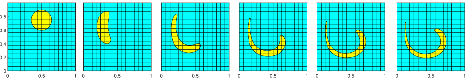
6.4 Domain with topological change

Finally we consider the domain having a topological change. Its boundary is given by the level set of the function

\displaystyle\phi({\bm{x}},t)=\min\{|{\bm{x}}-{\bm{c}}_{1}(t)|,|{\bm{x}}-{\bm{c}}_{2}(t)|\}-0.15,

where ${\bm{c}}_{1}(t)=[0.5,0.75-0.5t]^{\top}$ and ${\bm{c}}_{2}(t)=[0.5,0.25+0.5t]^{\top}$ are the centers of the two circles. The finial time is set by $T=1$ which satisfies $\phi({\bm{x}},0)=\phi({\bm{x}},T)$ . The evolution of the domain is shown in Fig. 7.

Table 7: Convergence rates for section 6.4 (

k=3

$h=\tau$	$e_{0}$	rate	$e_{1}$	rate
1/16	4.95e-05	-	6.37e-4	-
1/32	1.21e-05	2.03	1.52e-4	2.02
1/64	3.06e-06	1.98	4.36e-5	1.85
1/128	7.80e-07	1.98	1.09e-5	2.00

The exact solution is $u=\sin(\pi(x_{1}+t))\sin(\pi(x_{2}+t))$ . In the implementation of the ALE map, we choose ${\bm{g}}_{\eta}^{n,n-1}$ by the closet point mapping. Again we compute the $L^{2}$ - and $H^{1}$ -errors of the solution on the approximate domain $\Omega_{\eta}^{n}$ . Since the evolution of the domain is discontinuous, the assumption in (30) does not hold anymore. Table 7 shows that the convergence rate deteriorates into second order.

7 Conclusions

An arbitrary Lagrangian-Eulerian unfitted finite element (ALE-UFE) method has been presented for solving PDEs on time-varying domains. High-order convergence is obtained by adopting BDF schemes and ALE maps for time integration and unfitted finite element method for spatial discretization. The method is applied to various models, including a varying interface problem, a PDE-domain coupled problem, and a problem with topologically changing domain. The ALE-UFE method has the potential for solving a variety of moving-domain problems, such as fluid dynamics and FSI problems. These will be our future work.

Appendix A Useful estimates of the ALE mapping ${\bm{X}}^{n,n-1}$

Lemma A.1.

Suppose ${\bm{g}}^{n,n-1}({\bm{x}})={\bm{X}}_{F}(t_{n-1};t_{n},{\bm{x}})$ and ${\bm{X}}_{F}$ is given by (2). The Jacobi matrices $\mathbb{J}^{n,n-i}=\partial_{{\bm{x}}}{\bm{X}}^{n,n-i}$ , $1\leq i\leq k$ , of ALE maps admit

\|\mathbb{J}^{n,n-i}-\mathbb{I}\|_{L^{\infty}(\Omega^{n})}\lesssim\tau,\quad\|{\bm{w}}_{k}^{n}({\bm{x}},t_{n})\|\lesssim\infty.

Proof.

For ease of notation, we write ${\bm{d}}_{\bm{X}}={\bm{X}}^{n,n-1}-{\bm{X}}^{n,n}$ . Then (4) implies

\displaystyle-\Delta{\bm{d}}_{\bm{X}}=\textbf{0}\quad\text{in}\;\Omega^{n},\qquad{\bm{d}}_{\bm{X}}={\bm{g}}^{n,n-1}-{\bm{g}}^{n,n}\quad\text{on}\;\Gamma^{n}.

Since ${\bm{g}}^{n,n}={\bm{I}}$ and both $\Gamma^{n}$ and ${\bm{v}}$ are $C^{r}$ -smooth, we have $\|{\bm{g}}^{n,n-1}-{\bm{g}}^{n,n}\|_{{\bm{H}}^{r}(\Gamma^{n})}\lesssim\tau$ . The regularity result of elliptic equations yields

\left\|{{\bm{d}}_{\bm{X}}}\right\|_{{\bm{H}}^{r+1/2}(\Omega^{n})}\leq C\left\|{{\bm{g}}^{n,n-1}-{\bm{g}}^{n,n}}\right\|_{{\bm{H}}^{r}(\Gamma^{n})}\lesssim\tau.

(48)

Using ${\bm{X}}^{n,n}={\bm{I}}$ , Sobolev’s inequality, and (48), we find that

\|{\mathbb{J}^{n,n-1}-\mathbb{I}}\|_{{\bm{L}}^{\infty}(\Omega^{n})}=\|{{\bm{d}}_{\bm{X}}}\|_{{\bm{W}}^{1,\infty}(\Omega^{n})}\lesssim\|{{\bm{d}}_{\bm{X}}}\|_{{\bm{H}}^{r+1/2}(\Omega^{n})}\lesssim\tau.

By (5) and the chain rule, we obtain $\|{\mathbb{J}^{n,n-i}-\mathbb{I}}\|_{{\bm{L}}^{\infty}(\Omega^{n})}\lesssim\tau$ for $2\leq i\leq k$ .

From the definition of ${\bm{w}}^{n}_{k}$ in (7), a simple calculation gives

{\bm{w}}_{k}^{n}({\bm{x}},t_{n})|_{\Gamma^{n}}=\sum_{i=0}^{k}(l_{n}^{i})^{\prime}(t_{n}){\bm{X}}^{n,n-i}|_{\Gamma^{n}}=\frac{1}{\tau}\sum_{i=0}^{k}\lambda_{i}^{k}{\bm{X}}^{n,n-i}|_{\Gamma^{n}}=\frac{1}{\tau}\sum_{i=0}^{k}\lambda_{i}^{k}{\bm{g}}^{n,n-i},

where $\lambda_{i}^{k}$ are the coefficients of BDF- $k$ . Clearly ${\bm{w}}_{k}^{n}({\bm{x}},t_{n})|_{\Gamma^{n}}$ is an approximation to $\partial_{t}{\bm{X}}_{F}(t;t_{n},\cdot)|_{t=t_{n}}$ . It is easy to see from (4) that

-\Delta{\bm{w}}^{n}_{k}({\bm{x}},t_{n})=0\quad\text{in}\;\;\Omega^{n},\qquad{\bm{w}}^{n}_{k}({\bm{x}},t_{n})=\tau^{-1}\sum_{i=0}^{k}\lambda_{i}^{k}{\bm{g}}^{n,n-i}\quad\text{on}\;\;\Gamma^{n}.

(49)

By Sobolev’s inequalities and regularity theories of elliptic equations, we obtain

\displaystyle\|{\bm{w}}^{n}_{k}(t_{n})\|_{{\bm{L}}^{\infty}(\Omega^{n})}\lesssim\frac{1}{\tau}\Big{\|}\sum_{i=0}^{k}\lambda_{i}^{k}{\bm{g}}^{n,n-i}\Big{\|}_{{\bm{H}}^{r}(\Gamma^{n})}\lesssim\|\partial_{t}{\bm{X}}_{F}(t;t_{n},\cdot)|_{t=t_{n}}\|_{{\bm{H}}^{r}(\Gamma^{n})}.

∎

Since the computations and numerical analysis are performed on the approximate domain $\Omega_{\eta}^{n}$ , which is different from the exact one $\Omega^{n}$ in general, we have to extend ${\bm{X}}^{n,n-1}$ from $\Omega^{n}$ to the fictitious domain $\tilde{\Omega}^{n}$ .

Lemma A.2.

There exits an extension of ${\bm{X}}^{n,n-1}\in{\bm{H}}^{r+1/2}(\Omega^{n})$ , denoted by $\tilde{\bm{X}}^{n,n-1}\in{\bm{H}}^{r+1/2}(\tilde{\Omega}^{n})$ , such that

\tilde{\bm{X}}^{n,n-1}|_{\Omega^{n}}={\bm{X}}^{n,n-1},\qquad\|\tilde{\bm{X}}^{n,n-1}\|_{{\bm{H}}^{r+1/2}(\tilde{\Omega}^{n})}\leq\infty.

(50)

Moreover, the Jacobi matrix $\tilde{\mathbb{J}}^{n,n-1}=\partial_{{\bm{x}}}\tilde{{\bm{X}}}^{n,n-1}$ satisfies

\tilde{\mathbb{J}}^{n,n-1}|_{\Omega^{n}}=\mathbb{J}^{n,n-1},\qquad\|\tilde{\mathbb{J}}^{n,n-1}-\mathbb{I}\|_{\mathbb{L}^{\infty}(\tilde{\Omega}^{n})}\lesssim\tau.

Proof.

By the Sobolev extension theorem and (48), there exits an extension of ${\bm{d}}_{{\bm{X}}}$ , denoted by $\widetilde{{\bm{d}}_{{\bm{X}}}}\in{\bm{H}}^{r+1/2}(\tilde{\Omega}^{n})$ , such that

\widetilde{{\bm{d}}_{{\bm{X}}}}|_{\Omega^{n}}={\bm{d}}_{\bm{X}},\qquad\|\widetilde{{\bm{d}}_{\bm{X}}}\|_{{\bm{H}}^{r+1/2}(\tilde{\Omega}^{n})}\lesssim\|{\bm{d}}_{\bm{X}}\|_{{\bm{H}}^{r+1/2}(\Omega^{n})}\lesssim\tau.

(51)

Then the extension of ${\bm{X}}^{n,n-1}$ is defined by $\tilde{{{\bm{X}}}}^{n,n-1}:={\bm{I}}+\tau\widetilde{{\bm{d}}_{\bm{X}}}$ . It follows that

\tilde{{\bm{X}}}^{n,n-1}|_{\Omega^{n}}={{\bm{X}}}^{n,n-1},\qquad\|\tilde{{\bm{X}}}^{n,n-1}\|_{{\bm{H}}^{r+\frac{1}{2}}(\tilde{\Omega}^{n})}\lesssim\text{area}(D)+\tau.

(52)

Since $r\geq k+1\geq 3$ , from Sobolev’s inequality and (51), for $\mu=0$ , $1$ , we get

\|\tilde{{\bm{X}}}^{n,n-1}-{\bm{I}}\|_{{\bm{W}}^{\mu,\infty}(\tilde{\Omega}^{n})}\lesssim\tau\|\widetilde{{{\bm{d}}}_{{\bm{X}}}}\|_{{\bm{H}}^{2+\mu}(\tilde{\Omega}^{n})}\lesssim\tau^{2}.

(53)

This implies $\big{\|}\tilde{\mathbb{J}}^{n,n-1}-\mathbb{I}\big{\|}_{\mathbb{L}^{\infty}(\tilde{\Omega}^{n})}\lesssim\tau$ by noting $\tilde{\mathbb{J}}^{n,n-1}=\partial_{{\bm{x}}}\tilde{\bm{X}}^{n,n-1}$ . ∎

Appendix B Useful estimates of the discrete ALE map ${\bm{X}}_{h}^{n,n-i}$

Lemma B.1.

Let $\mathbb{J}_{h}^{n,n-1}:=\partial_{{\bm{x}}}{\bm{X}}_{h}^{n,n-1}$ be the Jacobi matrix of ${\bm{X}}_{h}^{n,n-1}$ . Upon hidden constants independent of $\tau,h,n$ , and $\eta$ , there hold

\|{\mathbb{J}_{h}^{n,n-1}-\mathbb{I}}\|_{\mathbb{L}^{\infty}(\tilde{\Omega}^{n})}\lesssim\tau,\qquad\|{{\bm{X}}_{h}^{n,n-1}-\tilde{\bm{X}}^{n,n-1}}\|_{{\bm{L}}^{\infty}(\tilde{\Omega}^{n})}\lesssim\tau^{k-1/2}.

(54)

Proof.

Since $\Omega_{\eta}^{n}\neq\Omega^{n}$ , multiplying both sides of (4) by ${\bm{v}}_{h}\in{\bm{V}}(k,\mathcal{T}_{h}^{n})$ and using $\tilde{\bm{X}}^{n,n-1}\in{\bm{H}}^{r+1/2}(\tilde{\Omega}^{n})\subset H^{k+1}(\tilde{\Omega}^{n})$ , we have

\mathcal{A}_{h}^{n}(\tilde{\bm{X}}^{n,n-1},{\bm{v}}_{h})=-(\Delta\tilde{{\bm{X}}}^{n,n-1},{\bm{v}}_{h})_{\Omega_{\eta}^{n}\backslash\Omega^{n}}+\mathcal{F}_{\Gamma_{\eta}^{n}}(\tilde{\bm{X}}^{n,n-1},{\bm{v}}_{h}).

(55)

For convenience, let $\mathcal{I}_{h}^{n}$ be the Lagrange interpolation operator and define

{\bm{e}}={\bm{X}}_{h}^{n,n-1}-\tilde{\bm{X}}^{n,n-1},\;\bm{\xi}_{h}={\bm{X}}_{h}^{n,n-1}-\mathcal{I}_{h}^{n}\tilde{\bm{X}}^{n,n-1},\;\bm{\eta}=\mathcal{I}_{h}^{n}\tilde{\bm{X}}^{n,n-1}-\tilde{\bm{X}}^{n,n-1}.

It is easy to see that ${\bm{e}}=\bm{\xi}_{h}+\bm{\eta}$ . Subtracting (55) from (19), one has

\displaystyle\mathcal{A}_{h}^{n}({\bm{e}},{\bm{v}}_{h})=(\Delta\tilde{{\bm{X}}}^{n,n-1},{\bm{v}}_{h})_{\Omega_{\eta}^{n}\backslash\Omega^{n}}+\mathcal{F}_{\Gamma_{\eta}^{n}}({\bm{g}}_{\eta}^{n,n-1}-\tilde{\bm{X}}^{n,n-1},{\bm{v}}_{h}).

(56)

For any ${\bm{v}}_{h}\in{\bm{V}}(k,\mathcal{T}_{h}^{n})$ , Poincar $\acute{\text{e}}$ inequality and (28) show

\left\|{{\bm{v}}_{h}}\right\|_{{\bm{L}}^{2}({\tilde{\Omega}^{n}})}\lesssim{\left|{{\bm{v}}_{h}}\right|}_{{\bm{H}}^{1}({\tilde{\Omega}^{n}})}+\mathscr{J}_{0}^{n}({\bm{v}}_{h},{\bm{v}}_{h})\lesssim\left\|\left|{{\bm{v}}_{h}}\right|\right\|_{\mathcal{T}_{h}^{n}}.

(57)

Since $\text{area}(\Omega_{\eta}^{n}\backslash\Omega^{n})=\tau^{k+1}$ , by [21, Lemma A4] and (57), we have

\displaystyle(\Delta\tilde{{\bm{X}}}^{n,n-1},{\bm{v}}_{h})_{\Omega_{\eta}^{n}\backslash\Omega^{n}}

\displaystyle\lesssim\tau^{k+1}\|{\tilde{\bm{X}}^{n,n-1}}\|_{{\bm{H}}^{3}(\tilde{\Omega}^{n})}\||{{\bm{v}}_{h}}|\|_{\mathcal{T}_{h}^{n}}.

(58)

Since the approximate boundary satisfies $\text{dist}(\Gamma^{n},\Gamma_{\eta}^{n})\lesssim\tau^{k+1}$ , and ${\bm{g}}_{\eta}^{n,n-1}$ is the $(k+1)^{\text{th}}$ -order approximation to ${\bm{g}}^{n,n-1}$ , there holds

\|{\bm{g}}_{\eta}^{n,n-1}-\tilde{\bm{X}}^{n,n-1}\|_{L^{2}(\Gamma_{\eta}^{n})}\lesssim\;\tau^{k+1}.

(59)

From the trace inequality, inverse estimate, and (59), we have

\displaystyle\mathcal{F}_{\Gamma_{\eta}^{n}}({\bm{X}}_{\tau}^{n,n-1}-\tilde{\bm{X}}^{n,n-1},{\bm{v}}_{h})\lesssim\tau^{k+\frac{1}{2}}\||{{\bm{v}}_{h}}|\|_{\mathcal{T}_{h}^{n}}.

(60)

Insert (58) and (60) into (56). By Lemma 3.8 and interpolation error estimates, we obtain

\displaystyle\||{\bm{\xi}_{h}}|\|^{2}_{\mathcal{T}_{h}^{n}}\lesssim\mathscr{A}_{h}^{n}(\bm{\xi}_{h},\bm{\xi}_{h})=\mathcal{A}_{h}^{n}({\bm{e}},\bm{\xi}_{h})-\mathcal{A}_{h}^{n}(\bm{\eta},\bm{\xi}_{h})\lesssim(\tau^{k+\frac{1}{2}}+h^{k})\||{\bm{\xi}_{h}}|\|_{\mathcal{T}_{h}^{n}}.

(61)

Thus together with (28) and (61), one has

|{\bm{\xi}_{h}}|_{{\bm{H}}^{1}(\tilde{\Omega}^{n})}\lesssim\||{\bm{\xi}_{h}}|\|_{\mathcal{T}_{h}^{n}}\lesssim h^{k}+\tau^{k+\frac{1}{2}}.

(62)

These yield $|{{\bm{e}}}|_{{\bm{H}}^{1}(\tilde{\Omega}^{n})}\lesssim h^{k}+\tau^{k+\frac{1}{2}}$ . Since $\|{\tilde{\bm{X}}^{n,n-1}}\|_{{\bm{W}}^{k,\infty}(\tilde{\Omega}^{n})}\lesssim\|{\tilde{\bm{X}}^{n,n-1}}\|_{{\bm{H}}^{r+\frac{1}{2}}(\tilde{\Omega}^{n})}$ , inverse estimates imply

\displaystyle\|{{\bm{e}}}\|_{{\bm{W}}^{1,\infty}(\tilde{\Omega}^{n})}\lesssim h^{-1}\|{\bm{\xi}_{h}}\|_{{\bm{H}}^{1}(\tilde{\Omega}^{n})}+h^{k-1}\|{\tilde{\bm{X}}^{n,n-1}}\|_{{\bm{H}}^{r+\frac{1}{2}}(\tilde{\Omega}^{n})}\lesssim h^{k-1}+\tau^{k-\frac{1}{2}}.

(63)

Let $\mathbb{J}_{h}^{n,n-1}=\partial_{{\bm{x}}}\tilde{\bm{X}}_{h}^{n,n-1}$ . From (63) and (53), we have

\displaystyle\|{\mathbb{J}_{h}^{n,n-1}-\mathbb{I}}\|_{{\bm{L}}^{\infty}(\tilde{\Omega}^{n})}

\displaystyle\leq\|{\mathbb{J}_{h}^{n,n-1}-\tilde{\mathbb{J}}^{n,n-1}}\|_{{\bm{L}}^{\infty}(\tilde{\Omega}^{n})}+\|{\tilde{\mathbb{J}}^{n,n-1}-\mathbb{I}}\|_{{\bm{L}}^{\infty}(\tilde{\Omega}^{n})}\leq\|{{\bm{e}}}\|_{{\bm{W}}^{1,\infty}(\tilde{\Omega}^{n})}+\tau\|{{\bm{X}}^{n,n-1}}\|_{{\bm{H}}^{r+\frac{1}{2}}(\Omega^{n})}\lesssim\tau.

From Sobolev’s inequality and inverse estimates, for any $v_{h}\in H^{1}(\tilde{\Omega}^{n})$ , we get

\left\|{v_{h}}\right\|_{L^{\infty}({\tilde{\Omega}^{n}})}\lesssim\left\|{v_{h}}\right\|_{W^{1,4}(\tilde{\Omega}^{n})}\lesssim h^{-\frac{1}{2}}{\left\|{v_{h}}\right\|}_{H^{1}({\tilde{\Omega}^{n}})}.

(64)

Moreover, it yields from (57), (62), (64) that

	$\displaystyle\left\\|{{\bm{e}}}\right\\|_{{\bm{L}}^{\infty}(\tilde{\Omega}^{n})}$	$\displaystyle\leq\left\\|{\bm{\xi}_{h}}\right\\|_{{\bm{L}}^{\infty}(\tilde{\Omega}^{n})}+\left\\|{\bm{\eta}}\right\\|_{{\bm{L}}^{\infty}(\tilde{\Omega}^{n})}\lesssim h^{-\frac{1}{2}}{\left\\|{\bm{\xi}_{h}}\right\\|}_{H^{1}({\tilde{\Omega}^{n}})}+h^{k}\left\\|{{\bm{X}}^{n,n-1}}\right\\|_{{\bm{W}}^{k,\infty}(\tilde{\Omega}^{n})}$
		$\displaystyle\lesssim h^{-\frac{1}{2}}\left\\|\left\|{\bm{\xi}_{h}}\right\|\right\\|_{\mathcal{T}_{h}^{n}}+h^{k}\lesssim h^{k-\frac{1}{2}}+h^{-\frac{1}{2}}\tau^{k+\frac{1}{2}}.$

The proof is finished by assuming $h=O(\tau)$ . ∎

Corollary B.2.

Let ${\bm{w}}^{n}_{k,h}$ be defined in (24) and write $\mathbb{J}_{h}^{n,n-i}:=\partial_{{\bm{x}}}{\bm{X}}^{n,n-i}_{h}$ and $\mathbb{J}_{h}^{n-i,n}:=(\mathbb{J}_{h}^{n,n-i})^{-1}$ for $1\leq i\leq k$ . Then $\|{\bm{w}}_{k,h}^{n}\|_{{\bm{L}}^{\infty}(\Omega_{\eta}^{n})}\lesssim\left\|{{\bm{w}}^{n}_{k}}\right\|_{{\bm{H}}^{r+1/2}(\Omega^{n})}$ and

	$\displaystyle\\|\mathbb{J}_{h}^{n,n-i}-\mathbb{I}\\|_{\mathbb{L}^{\infty}(\tilde{\Omega}^{n})}\lesssim\tau,\hskip 54.06023pt\operatorname{det}(\mathbb{J}_{h}^{n,n-i})=1+O(\tau),$		(65)
	$\displaystyle\\|{\mathbb{J}_{h}^{n-i,n}-\mathbb{I}}\\|_{\mathbb{L}^{\infty}({\bm{X}}_{h}^{n,n-i}(\Omega_{\eta}^{n}))}\lesssim\tau,\hskip 34.1433pt\operatorname{det}(\mathbb{J}_{h}^{n-i,n})=1+O(\tau).$		(66)

Proof.

Thanks to (13) and Lemma B.1, we have ${\bm{X}}_{h}^{n,n-j}(\Omega_{\eta}^{n})\subset\tilde{\Omega}^{n-j}$ for $1\leq j<k$ . So (25) is well defined. The proofs of (65)–(66) are direct consequences of (54). The stability of Sovolev extension shows that $\tilde{\bm{w}}^{n}_{k}=\frac{1}{\tau}\sum\limits_{i=0}^{k}\lambda_{i}^{k}\tilde{\bm{X}}^{n,n-i}$ satisfies

\tilde{\bm{w}}^{n}_{k}|_{\Omega^{n}}={\bm{w}}^{n}_{k},\qquad\|\tilde{\bm{w}}^{n}_{k}\|_{{\bm{H}}^{r+1/2}(\tilde{\Omega}^{n})}\lesssim\|{\bm{w}}^{n}_{k}\|_{{\bm{H}}^{r+1/2}(\Omega^{n})}.

Using Lemma B.1, we have

\|{\bm{w}}_{k,h}^{n}-\tilde{\bm{w}}^{n}_{k}\|_{{\bm{L}}^{\infty}(\Omega_{\eta}^{n})}\lesssim\tau^{-1}\sum_{i=0}^{k}\|{\bm{X}}_{h}^{n,n-i}-\tilde{\bm{X}}^{n,n-i}\|_{{\bm{L}}^{\infty}(\Omega_{\eta}^{n})}\lesssim\tau^{k-3/2}.

(67)

The proof is finished by the triangle inequality. ∎

Finally, we present estimates of the discrete ALE mapping by using Lemma B.1 and Corollary B.2.

Lemma B.3.

Assuming ${\bm{X}}_{h}^{n,n-1}$ satisfies (54) and $\tau=O(h)$ , there exits a constant $C$ independent of $n,\tau$ such that, for any $v_{h}\in V(k,\mathcal{T}_{h}^{n-i})$ , and $\mu=0,1$ ,

$\displaystyle\\|{\nabla^{\mu}\big{(}v_{h}\circ{\bm{X}}_{h}^{n,n-i}\big{)}}\\|^{2}_{L^{2}(\Omega_{\eta}^{n})}$	$\displaystyle\leq\;\\|{\nabla^{\mu}(v_{h}\circ{\bm{X}}_{h}^{n-l,n-i})}\\|^{2}_{L^{2}(\Omega_{\eta}^{n-l})}+Ch\\|\nabla^{\mu}v_{h}\\|_{L^{2}(\tilde{\Omega}^{n-i})}^{2},$	(68)
$\displaystyle\\|{v_{h}\circ{\bm{X}}_{h}^{n,n-1}}\\|^{2}_{L^{2}(\Gamma_{\eta}^{n})}$	$\displaystyle\leq(1+C\tau)\left\\|{v_{h}}\right\\|_{L^{2}({\Gamma_{\eta}^{n-1}})}^{2}+C\tau^{k-1}{\left\\|{v_{h}}\right\\|}_{H^{1}({\tilde{\Omega}^{n-1}})}^{2},$	(69)
$\displaystyle\big{\|}{v_{h}\circ{\bm{X}}_{h}^{n,n-1}}\big{\|}^{2}_{H^{1}(\Gamma_{\eta}^{n})}$	$\displaystyle\lesssim h^{-1}{\left\|{v_{h}}\right\|}_{H^{1}({\tilde{\Omega}^{n-1}})}^{2}.$	(70)

Appendix C The stability of numerical solutions

Since the computational domain is time-varying, we have to deal with the issue that $u^{n-j}_{h}\notin V(k,\mathcal{T}^{n}_{h})$ for $1\leq j\leq k$ when proving the stability and convergence of the discrete solution. To overcome this difficulty, we introduce a modified Ritz projection operator $\mathcal{P}^{n}_{h}:Y(\Omega^{n}_{\eta})\to V(k,\mathcal{T}^{n}_{h})$ proposed in [21] which satisfies

\displaystyle\mathscr{A}^{n}_{h}(\mathcal{P}^{n}_{h}w,v_{h})=a^{n}_{h}(w,v_{h})\qquad\forall\,v_{h}\in V(k,\mathcal{T}^{n}_{h}),

(71)

where $Y(\Omega_{\eta}^{n}):=\big{\{}v\in H^{1}({\Omega^{n}_{\eta}}):\left\|\left|{v}\right|\right\|_{\Omega^{n}_{\eta}}<\infty\big{\}}$ . It satisfies

\displaystyle\left\|\left|{\mathcal{P}_{h}^{n}w}\right|\right\|_{\Omega_{\eta}^{n}}\lesssim\left\|\left|{w}\right|\right\|_{\Omega_{\eta}^{n}},\qquad\left\|{w-\mathcal{P}^{n}_{h}w}\right\|_{L^{2}({\Omega^{n}_{\eta}})}\lesssim h\left\|\left|{w}\right|\right\|_{\Omega^{n}_{\eta}},\quad\forall w\in Y(\Omega^{n}_{\eta}).

(72)

C.1 Proof of Theorem 3.9

Proof.

We only prove the theorem for $k=4$ . The proofs for other cases are similar. The rest of the proof is parallel to the proof of [21, Theorem 5.2], we just sketch the proof and omit details.

Step1: Selection of a particular test function. Write $\tilde{U}^{n-1,n}_{h}=\mathcal{P}^{n}_{h}(U^{n-1,n}_{h})$ . Since $U^{n-1,n}_{h}\notin V(k,\mathcal{T}^{n}_{h})$ , we choose $v_{h}=2u^{n}_{h}-\tilde{U}^{n-1,n}_{h}$ as a test function, the discrete problem for $k=4$ has the form

\sum_{i=1}^{5}\|\bm{\Psi}_{i}^{4}(\underline{{\bm{U}}_{h}^{n}})\|_{L^{2}(\Omega^{n}_{\eta})}^{2}-\sum_{i=1}^{4}\|\bm{\Phi}_{i}^{4}(\underline{{\bm{U}}_{h}^{n}})\|^{2}_{L^{2}(\Omega^{n}_{\eta})}+\tau\mathscr{A}^{n}_{h}(u_{h}^{n},v_{h})+\tau\mathscr{B}_{h}^{n}(u_{h}^{n},v_{h})=\tau R^{n}_{1}+R^{n}_{2},

(73)

where $\mathscr{B}_{h}^{n}(u_{h}^{n},v_{h})=(-\nabla{\bm{w}}_{k,h}^{n}\cdot\nabla u_{h}^{n},v_{h})_{\Omega_{\eta}^{n}}$ , we have used [18, Section 2 and Appendix A], and

	$\displaystyle\bm{\Psi}^{4}_{i}\big{(}\underline{{\bm{U}}^{n}_{h}}\big{)}=\sum_{j=1}^{i}c_{i,j}^{4}U_{h}^{n+1-j,n},\quad\bm{\Phi}_{i}^{4}\big{(}\underline{{\bm{U}}^{n}_{h}}\big{)}=\sum_{j=1}^{i}c_{i,j}^{4}U_{h}^{n-j,n},$
	$\displaystyle R^{n}_{1}=\big{(}f^{n},2u^{n}_{h}-\tilde{U}^{n-1,n}_{h}\big{)}_{\Omega^{n}_{\eta}},\quad R^{n}_{2}=\big{(}\Lambda^{4}\underline{{\bm{U}}_{h}^{n}},\tilde{U}^{n-1,n}_{h}-U^{n-1,n}_{h}\big{)}_{\Omega^{n}_{\eta}}.$

The trace inequality and inverse estimates show $\|\partial_{\bm{n}}u^{n}_{h}\|_{L^{2}(\Gamma^{n}_{\eta})}\lesssim h^{-\frac{1}{2}}|u^{n}_{h}|_{H^{1}(\tilde{\Omega}^{n})}$ . For any $\varepsilon\in(0,1)$ , by the definitions of $\mathcal{P}^{n}_{h}$ and the Cauchy-Schwarz inequality, one has

	$\displaystyle\mathscr{A}^{n}_{h}(u_{h}^{n},\,2u_{h}^{n}-\tilde{U}^{n-1,n}_{h})=\,2\mathscr{A}^{n}_{h}(u_{h}^{n},u_{h}^{n})-a^{n}_{h}(u_{h}^{n},U^{n-1,n}_{h})$
	$\displaystyle\,\geq\frac{3}{2}\left\\|\left\|{u_{h}^{n}}\right\|\right\\|^{2}_{\mathcal{T}_{h}^{n}}-\frac{5}{2\varepsilon h}\\|{u^{n}_{h}}\\|^{2}_{L^{2}(\Gamma^{n}_{\eta})}-C\varepsilon\|{u^{n}_{h}}\|^{2}_{H^{1}(\tilde{\Omega}^{n})}-\frac{1}{2}\|{U^{n-1,n}_{h}}\|^{2}_{H^{1}(\Omega^{n}_{\eta})}-\frac{\varepsilon h}{2}\|{U_{h}^{n-1,n}}\|^{2}_{H^{1}(\Gamma_{\eta}^{n})}-\frac{\gamma_{0}+\varepsilon^{-1}}{2h}\\|{U^{n-1,n}_{h}}\\|^{2}_{L^{2}(\Gamma^{n}_{\eta})}.$		(74)

Since ${\bm{w}}_{k,h}^{n}$ is bounded with $C_{w}=\|{\bm{w}}_{k,h}^{n}\|_{{\bm{L}}^{\infty}(\Omega_{\eta}^{n})}$ and $U^{n-1,n}_{h}\in Y(\Omega^{n}_{\eta})$ , we infer from (72) and the Cauchy-Schwarz inequality that

	$\displaystyle\mathscr{B}_{h}^{n}(u_{h}^{n},v_{h})\leq\,$	$\displaystyle\frac{\|{u_{h}^{n}}\|^{2}_{H^{1}(\Omega_{\eta}^{n})}}{4}+8C_{w}^{2}\big{(}\\|{u_{h}^{n}}\\|^{2}_{L^{2}(\Omega_{\eta}^{n})}+\\|{U_{h}^{n-1,n}}\\|^{2}_{L^{2}(\Omega_{\eta}^{n})}+Ch^{2}\\|\|{U_{h}^{n-1,n}}\\|\|_{\Omega_{\eta}^{n}}^{2}\big{)},$
	$\displaystyle R^{n}_{1}\leq\,$	$\displaystyle 2\\|{f^{n}}\\|^{2}_{L^{2}(\Omega^{n}_{\eta})}+\\|{u^{n}_{h}}\\|^{2}_{L^{2}(\Omega^{n}_{\eta})}+\\|{U^{n-1,n}_{h}}\\|^{2}_{L^{2}(\Omega^{n}_{\eta})}+Ch^{2}\\|\|{U^{n-1,n}_{h}}\\|\|_{\Omega^{n}_{\eta}}^{2},$
	$\displaystyle R^{n}_{2}\leq\,$	$\displaystyle C\tau\varepsilon^{-1}\sum_{j=0}^{4}\\|{U^{n-j,n}_{h}}\\|^{2}_{L^{2}(\Omega^{n}_{\eta})}+\frac{\tau\varepsilon}{4}\\|\|{U^{n-1,n}_{h}}\\|\|_{\Omega^{n}_{\eta}}^{2}.$

Step2: Estimate of $\Phi_{i}^{4}(\underline{{\bm{U}}_{h}^{n}})$ . We deduce from the inverse estimates and Lemma B.3 that

$\displaystyle\\|{\nabla^{\mu}U^{n-j,n}_{h}}\\|^{2}_{{\bm{L}}^{2}(\Omega^{n}_{\eta})}\leq\,$	$\displaystyle\\|{\nabla^{\mu}u^{n-j}_{h}}\\|^{2}_{{\bm{L}}^{2}(\Omega^{n-j}_{\eta})}+C\tau\\|{\nabla^{\mu}u^{n-j}_{h}}\\|^{2}_{{\bm{L}}^{2}(\tilde{\Omega}^{n-j})},\quad\mu=0,1,$	(75)
$\displaystyle\\|{U^{n-1,n}_{h}}\\|^{2}_{L^{2}(\Gamma^{n}_{\eta})}\leq\,$	$\displaystyle(1+C\tau)\\|{u^{n-1}_{h}}\\|^{2}_{L^{2}(\Gamma^{n-1}_{\eta})}+C\tau^{3}\\|{u^{n-1}_{h}}\\|^{2}_{H^{1}(\tilde{\Omega}^{n-1})},$	(76)
$\displaystyle\|{U_{h}^{n-1,n}}\|_{H^{1}(\Gamma_{\eta}^{n})}\lesssim\,$	$\displaystyle h^{-1/2}\\|{u_{h}^{n-1}}\\|_{H^{1}(\tilde{\Omega}^{n-1})}.$	(77)

Note that $\bm{\Phi}_{i}^{4}\big{(}\underline{{\bm{U}}_{h}^{n}}\big{)}=\bm{\Psi}_{i}^{4}\big{(}\underline{{\bm{U}}_{h}^{n-1}}\big{)}\circ{\bm{X}}_{h}^{n,n-1}$ . It is easy to see from Lemma B.3 that

\displaystyle\|{\bm{\Phi}_{i}^{4}(\underline{{\bm{U}}_{h}^{n}})}\|^{2}_{L^{2}(\Omega_{\eta}^{n})}\leq\,\|{\bm{\Psi}_{i}^{4}(\underline{{\bm{U}}_{h}^{n-1}})}\|^{2}_{L^{2}(\Omega_{\eta}^{n-1})}+C\tau\sum_{j=1}^{i}\|{u_{h}^{n-j}}\|^{2}_{L^{2}(\tilde{\Omega}^{n-j})}.

(78)

Step3: Application of Gronwall’s inequality. Substituting (74)–(78) into (73), using $O(h)=\tau\leq h\ll\varepsilon\ll 1$ , $C_{w}^{2}h\leq\varepsilon$ , applying (28), and taking the sum of the inequalities over $4\leq n\leq m$ , we end up with

		$\displaystyle\sum_{i=1}^{4}\\|{\bm{\Psi}_{i}^{4}(\underline{{\bm{U}}_{h}^{m}})}\\|^{2}_{L^{2}(\Omega_{\eta}^{m})}+\frac{3}{2}\tau\sum_{n=4}^{m}\\|\|{u_{h}^{n}}\\|\|^{2}_{\mathcal{T}_{h}^{n}}$
	$\displaystyle\leq\,$	$\displaystyle\sum_{n=4}^{m}\tau(1+C\varepsilon)\\|\|u_{h}^{n}\\|\|_{\mathcal{T}_{h}^{n}}^{2}+\sum_{n=4}^{m}\tau\Big{[}C\\|{u^{n}_{h}}\\|^{2}_{L^{2}(\Omega^{n}_{\eta})}+2\\|{f^{n}}\\|^{2}_{L^{2}(\Omega^{n}_{\eta})}+\big{(}\frac{6+C\tau}{2\varepsilon h}-\frac{\gamma_{0}}{2h}\big{)}\\|u_{h}^{n}\\|_{L^{2}(\Gamma_{\eta}^{n})}^{2}\Big{]}+C_{0},$

after careful calculation, where $C_{0}$ is related to the initial solutions, $C_{0}=C\sum_{i=0}^{3}\tau\||{u^{i}_{h}}\||^{2}_{\mathcal{T}_{h}^{i}}+\sum_{i=1}^{4}\|{\bm{\Psi}_{i}^{4}(\underline{{\bm{U}}_{h}^{3}})}\|^{2}_{L^{2}(\Omega^{3}_{\eta})}$ . From [18, Table 2.2], we know $\bm{\Psi}_{1}^{4}\big{(}\underline{{\bm{U}}_{h}^{m}}\big{)}=c^{4}_{1,1}u^{m}_{h}$ ( $c_{1,1}^{4}>0$ ). Finally, we choose $\varepsilon$ small enough such that $C\varepsilon<1/2$ and $\gamma_{0}$ large enough such that $\gamma_{0}\geq(6+C\tau)/\varepsilon$ . Then the proof is finished by using Gronwall’s inequality. ∎

References

[1] S. Adjerid and K. Moon, An immersed discontinuous Galerkin method for acoustic wave propagation in inhomogeneous media, SIAM J. Sci. Comput., 41 (2019), pp. A139–A162.
[2] A. M. Andrew, Level set methods and fast marching methods, Cambridge University Press, Cambridge, UK, 2 ed., 1999.
[3] U. M. Ascher and S. J. Ruuth, and B. T. Wetton, Implicit-explicit methods for time-dependent partial differential equations, SIAM J. Numer. Anal., 32(1995), pp. 797-823.
[4] E. Burman, S. Frei, and A. Massing, Eulerian time-stepping schemes for the non-stationary stokes equations on time-dependent domains, Numer. Math., 150 (2022), pp. 423–478.
[5] J. Donea, S. Giuliani, and J. P. Halleux, An arbitrary lagrangian-eulerian finite element method for transient dynamic fluid-structure interactions, Comput. Methods Appl. Mech. Engrg., 33 (1982), pp. 689–723.
[6] C. Farhat, P. Geuzaine, and C. Grandmont, The discrete geometric conservation law and the nonlinear stability of ALE schemes for the solution of flow problems on moving grids, J. Comput. Phys., 174 (2001), pp. 669–694.
[7] L. Formaggia and F. Nobile, A stability analysis for the arbitrary Lagrangian Eulerian formulation with finite elements, East-West J. Math., 7 (1999), pp. 105–132.
[8] T. P. Fries and A. Zilian, On time integration in the XFEM, Internat. J. Numer. Methods Engrg., 79 (2009), pp. 69–93.
[9] P. Geuzaine, C. Grandmont, and C. Farhat, Design and analysis of ALE schemes with provable second-order time-accuracy for inviscid and viscous flow simulations, J. Comput. Phys., 191 (2003), pp. 206–227.
[10] R. Guo, Solving parabolic moving interface problems with dynamical immersed spaces on unfitted meshes: fully discrete analysis, SIAM J. Numer. Anal., 59 (2021), pp. 797–828.
[11] J. Guzmán and M. Olshanskii, Inf-sup stability of geometrically unfitted Stokes finite elements, Math. Comp., 87 (2018), pp. 2091–2112.
[12] P. Hansbo, M. G. Larson, and S. Zahedi, Characteristic cut finite element methods for convection–diffusion problems on time dependent surfaces, Comput. Methods Appl. Mech. Engrg., 293 (2015), pp. 431–461.
[13] C. W. Hirt, A. A. Amsden, and J. L. Cook, An arbitrary lagrangian-eulerian computing method for all flow speeds, J. Comput. Phys., 14 (1974), pp. 227–253.
[14] T. J. Hughes, W. K. Liu, and T. K. Zimmermann, Lagrangian-Eulerian finite element formulation for incompressible viscous flows, Comput. Methods Appl. Mech. Engrg., 29 (1981), pp. 329–349.
[15] C. Lehrenfeld and M. Olshanskii, An Eulerian finite element method for PDEs in time-dependent domains, ESAIM Math. Model. Numer. Anal., 53 (2019), pp. 585–614.
[16] C. Lehrenfeld and A. Reusken, Analysis of a nitsche XFEM-DG discretization for a class of two-phase mass transport problems, SIAM J.Numer. Anal., 51 (2013), pp. 958–983.
[17] C. Y. Li, S. V. Garimella, and J. E. Simpson, Fixed-grid front-tracking algorithm for solidification problems, part I: Method and validation, Numerical Heat Transfer, Part B: Fundamentals, 43 (2003), pp. 117–141.
[18] J. Liu, Simple and efficient ALE methods with provable temporal accuracy up to fifth order for the Stokes equations on time varying domains, SIAM J. Numer. Anal., 51 (2013), pp. 743–772.
[19] Y. Lou and C. Lehrenfeld, Isoparametric unfitted BDF–finite element method for PDEs on evolving domains, SIAM J. Numer. Anal., 60 (2022), pp. 2069–2098.
[20] C. Ma, T. Tian, and W. Zheng, High-order unfitted characteristic finite element methods for moving interface problem of Oseen equations, J. Comput. Appl. Math., 425 (2023), 115028.
[21] C. Ma, Q. Zhang, and W. Zheng, A fourth-order unfitted characteristic finite element method for solving the advection-diffusion equation on time-varying domains, SIAM J. Numer. Anal., 60 (2022), pp. 2203–2224.
[22] C. Ma and W. Zheng, A fourth-order unfitted characteristic finite element method for free-boundary problems, J. Comput. Phys., 469 (2022), 111552.
[23] A. Masud and T. J. Hughes, A space-time Galerkin/least-squares finite element formulation of the Navier-Stokes equations for moving domain problems, Comput. Methods Appl. Mech. Engrg., 146 (1997), pp. 91–126.
[24] T. Richter, Fluid-structure interactions: models, analysis and finite elements, Springer, 2017.
[25] T. E. Tezduyar, M. Behr, S. Mittal, and J. Liou, A new strategy for finite element computations involving moving boundaries and interfaces—the deforming-spatial-domain/space-time procedure: II. computation of free-surface flows, two-liquid flows, and flows with drifting cylinders, Comput. Methods Appl. Mech. Engrg., 94 (1992), pp. 353–371.
[26] H. von Wahl and T. Richter, Error analysis for a parabolic PDE model problem on a coupled moving domain in a fully Eulerian framework, SIAM J. Numer. Anal., 61 (2023), pp. 286–314.
[27] H. von Wahl, T. Richter, and C. Lehrenfeld, An unfitted Eulerian finite element method for the time-dependent Stokes problem on moving domains, IMA J. Numer. Anal., 42 (2022), pp. 2505–2544.
[28] Q. Zhang, Fourth-and higher-order interface tracking via mapping and adjusting regular semianalytic sets represented by cubic splines, SIAM J. Sci. Comput., 40 (2018), pp. A3755–A3788.
[29] P. Zunino, Analysis of backward Euler/Extended finite element discretization of parabolic problems with moving interfaces, Comput. Methods Appl. Mech. Engrg., 258 (2013), pp. 152–165.

$\displaystyle\\|{\nabla^{\mu}\big{(}v_{h}\circ{\bm{X}}_{h}^{n,n-i}\big{)}}\\|^{2}_{L^{2}(\Omega_{\eta}^{n})}$	$\displaystyle\leq\;\\|{\nabla^{\mu}(v_{h}\circ{\bm{X}}_{h}^{n-l,n-i})}\\|^{2}_{L^{2}(\Omega_{\eta}^{n-l})}+Ch\\|\nabla^{\mu}v_{h}\\|_{L^{2}(\tilde{\Omega}^{n-i})}^{2},$	(68)
$\displaystyle\\|{v_{h}\circ{\bm{X}}_{h}^{n,n-1}}\\|^{2}_{L^{2}(\Gamma_{\eta}^{n})}$	$\displaystyle\leq(1+C\tau)\left\\|{v_{h}}\right\\|_{L^{2}({\Gamma_{\eta}^{n-1}})}^{2}+C\tau^{k-1}{\left\\|{v_{h}}\right\\|}_{H^{1}({\tilde{\Omega}^{n-1}})}^{2},$	(69)
$\displaystyle\big{\|}{v_{h}\circ{\bm{X}}_{h}^{n,n-1}}\big{\|}^{2}_{H^{1}(\Gamma_{\eta}^{n})}$	$\displaystyle\lesssim h^{-1}{\left\|{v_{h}}\right\|}_{H^{1}({\tilde{\Omega}^{n-1}})}^{2}.$	(70)

$\displaystyle\\|{\nabla^{\mu}U^{n-j,n}_{h}}\\|^{2}_{{\bm{L}}^{2}(\Omega^{n}_{\eta})}\leq\,$	$\displaystyle\\|{\nabla^{\mu}u^{n-j}_{h}}\\|^{2}_{{\bm{L}}^{2}(\Omega^{n-j}_{\eta})}+C\tau\\|{\nabla^{\mu}u^{n-j}_{h}}\\|^{2}_{{\bm{L}}^{2}(\tilde{\Omega}^{n-j})},\quad\mu=0,1,$	(75)
$\displaystyle\\|{U^{n-1,n}_{h}}\\|^{2}_{L^{2}(\Gamma^{n}_{\eta})}\leq\,$	$\displaystyle(1+C\tau)\\|{u^{n-1}_{h}}\\|^{2}_{L^{2}(\Gamma^{n-1}_{\eta})}+C\tau^{3}\\|{u^{n-1}_{h}}\\|^{2}_{H^{1}(\tilde{\Omega}^{n-1})},$	(76)
$\displaystyle\|{U_{h}^{n-1,n}}\|_{H^{1}(\Gamma_{\eta}^{n})}\lesssim\,$	$\displaystyle h^{-1/2}\\|{u_{h}^{n-1}}\\|_{H^{1}(\tilde{\Omega}^{n-1})}.$	(77)

A new framework of high-order unfitted finite element methods using ALE maps for moving-domain problems

Abstract

keywords:

1 Introduction

2 Flow maps

2.1 Forward boundary map

2.2 Backward flow map based on the ALE map

Remark 2.3.

3 The ALE-UFE method

3.1 The heat equation on a moving domain

3.2 Interface-tracking approximation

Remark 3.3.

3.4 Finite element spaces

3.5 Construction of an approximate ALE map

3.6 The fully discrete scheme

3.7 Well-posedness and error estimates

Theorem 3.8.

Theorem 3.9.

Theorem 3.10.

3.11 The ALE-UFE framework

4 A domain-PDE-coupled problem

4.1 Flow maps

4.2 Surface tracking algorithm via forward boundary map

4.3 Construction of an approximate ALE map

4.4 The discrete scheme

5 A two-phase problem

5.1 Finite element spaces

5.2 Discrete ALE map and fully discrete scheme

6 Numerical experiments

6.1 One-phase linear problem

6.2 Nonlinear problem

6.3 Two-phase flow

6.4 Domain with topological change

7 Conclusions

Appendix A Useful estimates of the ALE mapping 𝑿n,n−1{\bm{X}}^{n,n-1}

Lemma A.1.

Proof.

Lemma A.2.

Proof.

Appendix B Useful estimates of the discrete ALE map 𝑿hn,n−i{\bm{X}}_{h}^{n,n-i}

Lemma B.1.

Proof.

Corollary B.2.

Proof.

Lemma B.3.

Appendix C The stability of numerical solutions

C.1 Proof of Theorem 3.9

Proof.

References

Appendix A Useful estimates of the ALE mapping ${\bm{X}}^{n,n-1}$

Appendix B Useful estimates of the discrete ALE map ${\bm{X}}_{h}^{n,n-i}$