These authors should be nominated as the corresponding author. \equalcontThese authors should be nominated as the corresponding author.
[1]\surZhonglong Zheng \equalcontThese authors should be nominated as the corresponding author.
[1]\orgdivSchool of Computer Science and Technology, \orgnameZhejiang Normal University, \orgaddress\streetNo. 688 Yingbin Avenue, \cityJinhua, \postcode321004, \stateZhejiang, \countryChina
2]\orgdivSchool of Data Science and MOE Frontiers Center for Brain Science, \orgnameFudan University, \orgaddress\streetNo.220 Handan Road, \cityShanghai, \postcode200433, \stateShanghai, \countryChina
3]\orgdivFudan ISTBI-JNU Algorithm Centre for Brain inspired Intelligence, \orgnameZhejiang Normal University, \orgaddress\streetNo. 688 Yingbin Avenue, \cityJinhua, \postcode321004, \stateZhejiang, \countryChina
A New Formulation of Lipschitz Constrained With Functional Gradient Learning for GANs
Abstract
This paper introduces a promising alternative method for training Generative Adversarial Networks (GANs) on large-scale datasets with clear theoretical guarantees. GANs are typically learned through a minimax game between a generator and a discriminator, which is known to be empirically unstable. Previous learning paradigms have encountered mode collapse issues without a theoretical solution. To address these challenges, we propose a novel Lipschitz-constrained Functional Gradient GANs learning (Li-CFG) method to stabilize the training of GAN and provide a theoretical foundation for effectively increasing the diversity of synthetic samples by reducing the neighborhood size of the latent vector. Specifically, we demonstrate that the neighborhood size of the latent vector can be reduced by increasing the norm of the discriminator gradient, resulting in enhanced diversity of synthetic samples. To efficiently enlarge the norm of the discriminator gradient, we introduce a novel -centered gradient penalty that amplifies the norm of the discriminator gradient using the hyper-parameter . In comparison to other constraints, our method enlarging the discriminator norm, thus obtaining the smallest neighborhood size of the latent vector. Extensive experiments on benchmark datasets for image generation demonstrate the efficacy of the Li-CFG method and the -centered gradient penalty. The results showcase improved stability and increased diversity of synthetic samples.
keywords:
Generative Adversarial Nets, Functional Gradient Methods, New Lipschitz Constraint, Synthesis Diversity
1 Introduction
GANs are designed to sample a random variable from a known distribution , approximating the underlying data distribution . This learning process is modeled as a minimax game where the generator and discriminator are iteratively optimized, as introduced by Goodfellow et al. [1]. The generator produces samples that mimic the true data distribution, while the discriminator distinguishes between the generated data and real data samples. Despite numerous remarkable efforts that have been made [2, 3], the GANs learning still suffers from training instability and mode collapse.
Recently, Composite Functional Gradient Learning (CFG), as proposed in Johnson and Zhang [4], has gained attention. CFG utilizes a strong discriminator and functional gradient learning for the generator, leading to convergent GAN learning theoretically and empirically. However, we have observed that there are still various hyper-parameters in CFG that may significantly impact the GAN learning process. Despite the advancements in stability, one still needs to carefully set these hyper-parameters to ensure a successful and well-trained GAN. Properly tuning these parameters remains an essential aspect of achieving optimal performance in GAN training. This issue hinders the widespread adoption of the CFG method for training GAN in real-world and large-scale datasets. One of the most effective mechanisms for addressing this issue for GAN training is the Lipschitz constraint, with the -centered gradient penalty introduced by Mescheder et al. [5] and the -centered gradient penalty introduced by Gulrajani et al. [3] being among the most well-known. Empirically, stable training of a GAN can result in more diverse synthesis results. However, the theoretical foundation for stable GAN training using the Lipschitz gradient penalty and generating diverse synthesis samples is still unclear. It is therefore important to develop a new theoretical framework that can account for the Lipschitz constraint of the discriminator and the diversity of synthesis samples.
To address these challenges, we propose Lipschitz Constrained Functional Gradient GANs Learning (Li-CFG), an improved version of CFG. We present a comparative analysis of our Li-CFG and CFG methods in Fig. 2 and Example. 1.1. Additionally, we emphasize the importance of diversity in synthetic samples through Fig. 1. Remarkably, as shown in Fig. 1, the horse images generated by Li-CFG display a more diverse range of gestures, colors, and textures in comparison to those produced by the CFG method. When synthetic samples lack diversity, they fail to capture essential image characteristics. While recent generative models have made notable progress in enhancing diversity, there remains a gap in providing comprehensive theoretical explanations for certain aspects.

Example 1.1.
Fig. 2 indicates the idea that too large degree of leads to an excessively small neighborhood of the latent vector which causes an untrained model, a too-small degree of lead to an overly large neighborhood of the latent vectors which cause a worse diversity, i.e., the blue dashed lines with a reasonable degree of lead to the best FID compared to the results of other colors, the green solid lines with a too large degree of lead to an untrained result and the red dashed lines with a too small degree of lead to a worse diversity. Training results with different of CFG method and Li-CFG, illustrating that FID result of CFG with different varying dramatically due to the unstable change of . However, the FID result of our Li-CFG with different varying more stable due to the smooth thanks to the gradient penalty. By controlling the degree of via changing the value of our -centered gradient penalty, we can adjust the neighborhood size of the latent vector and consequently influence the degree of diversity of synthetic samples.
Our key insight is the introduction of Lipschitz continuity, a robust form of uniform continuity, into CFG. This provides a theoretical basis showing that synthetic sample diversity can be enhanced by reducing the latent vector neighborhood size through a discriminator constraint. For simplicity and clarity, we will use latent N-size to denote the neighborhood size of the latent vector and constraint to refer to the discriminator constraint for the rest of the article. First, Li-CFG integrates the Lipschitz constraint into CFG to tackle instability in training under dynamic theory Second, we establish a theoretical link between the discriminator gradient norm and the latent N-size. By increasing the discriminator gradient norm, the latent N-size is reduced, thus enhancing the diversity of synthetic samples. Lastly, to efficiently adjust the discriminator gradient norm, we introduce a novel Lipschitz constraint mechanism, the -centered gradient penalty. This mechanism enables fine-tuning of the latent vector neighborhood size by varying the hyper-parameter . Through this approach, we aim to achieve more effective control over the discriminator gradient norm and further improve the diversity of generated samples.
We summarize the key contributions of this work as follows: (1) We introduce a novel Lipschitz constraint to CFG, the -centered gradient penalty, addressing the hyperparameter sensitivity in regression-based GAN training. Our Li-CFG method enables stable GAN training, producing superior results compared to traditional CFG. (2) We present a new perspective on analyzing the relationship between the discriminator constraint and synthetic sample diversity. To the best of our knowledge, we are the first to explore this relationship, demonstrating that our -centered gradient penalty allows for effective control of diversity during training. (3) Our empirical studies highlight the superiority of Li-CFG over CFG across a variety of datasets, including synthetic and real-world data such as MNIST, CIFAR10, LSUN, and ImageNet. In an ablation study, we show a trade-off between diversity and model trainability. Additionally, we demonstrate the generalizability of our -centered gradient penalty across multiple GAN models, achieving better results compared to existing gradient penalties.
2 Preliminary
To enhance readability, we provide definitions for frequently used mathematical symbols in our theory. For CFG and dynamic theory, the symbols will be explained in the respective sections.
Notation. represents a generator model that maps an element of the latent space to the image space , where the parameter of generator is denoted by . Here is a sample drawn from a low dimensional latent distribution . We will use and interchangeably to refer to the generator throughout this article.
represents a discriminator model that maps elements from the image space to the probability of belonging to real data distribution or the generated data distribution, where the parameter of generator is denoted by . is a sample drawn from real data distribution . consists of the scale value obtained from the outputs of the discriminator. The symbol in the CFG method, along with the notation used in both the gradient penalty and our neighborhood theory, all represent the discriminator.
We use to denote the gradient penalty. Furthermore, we use to denote the -centered Gradient Penalty, to denote the -centered Gradient Penalty and to denote the -centered Gradient Penalty. stands for the latent N-size of the corresponding gradient penalty. The symbol in the definition of our neighborhood method represents a small quantity in image space. It is distinct from the symbol used in our -centered GP method.
Composite Functional Gradient GANs. We follow the definition in CFG [6]. The CFG employs discriminator works as a logistic regression to differentiate real samples from synthetic samples. Meanwhile, it employs the functional compositions gradient to learn the generator as the following form
| (1) |
to obtain . The represents the number of steps in the generator used to approximate the distribution of real data samples. Each is a function to be estimated from data. is a residual which gradually move the generated samples of step towards the step . guarantees that the distance between the latent distribution and the real data distribution will gradually decrease until it reaches zero, and the is a small step size.
To simplify the analysis of this problem, we first transform the discrete M into the continuous M. First, we transform the Eq. (1) into by setting , where is a small time step. By letting , we have a generator that evolves continuously in time that satisfies an ordinary differential equation
The goal is to learn from data so that the probability density of , which continuously evolves by Eq. (1), becomes close to the density of real data as continuously increases. To measure the ‘closeness’, we use denotes a distance measure between two distributions:
where is a pre-defined function so that satisfies if and only if and for any probability density function .
From the above equation, we will derive the choice of that guarantees that transformation Eq. (1) can always reduce . Let be the probability density of random variable . Let . Then we have
With this definition of , we aim to keep that is negative, so that the distance decreases. To achieve this goal, we choose to be:
| (2) |
where is an arbitrary scaling factor. is a vector function such that and if and only if . Here are two examples: and .
With this choice of , we obtain
| (3) |
that is, the distance is guaranteed to decrease unless the equality holds. Moreover, this implies that we have . (Otherwise, would keep going down and become negative as increases, but by definition.) For simplicity, we omit the subscript in the following empirical settings.
Let us consider a case where the distance measure is an -divergence. With a convex function such that and that is strictly convex at defined by
is called -divergence. Here we focus on a special case where is twice differentiable and strongly convex so that the second order derivative of , denoted here by , is always positive. For instance, when we consider the KL divergence, can be represented by , in which case and . On the other hand, if we consider the reverse KL divergence, can be represented as , in which case and .
With this definition of function and as -divergence setting, the value of should to be
| (4) |
where is an arbitrary scaling factor, , , when is KL-divergence and when , which is the analytic solution of the CFG discriminator.
Empirically, we define the function in Eq. (4) as . The can be computed as
| (5) |
where we have an arbitrary scaling factor , a KL-divergence function , and . Since , it can be absorbed into the . So the value of is always greater than 0. For simplicity, we directly regard as the scaling factor and set it to a fixed value as a hyper-parameter. We also demonstrate the results of different values in the Fig. 2.
Gradient Penalty for GANs. Let us work with the most commonly used WGAN-GP [3]. Its regularization term is commonly referred to as
| (6) |
where is sampled uniformly on the line segment between two random points vector . The notation of presents the regularization term of the generator with weight and the discriminator with weight . The notion of is a coefficient that controls the magnitude of regularization. The value of is always empirically set to 1. We call it -centered GP or -centered GP. The other solution is referred to as the -centered GP method, proposed by Roth et al. [7] and Mescheder et al. [5]. The formulation is
| (7) |
where is sampled uniformly on the line segment between two random points vector like WGAN-GP.
When integrating the gradient penalty into the GAN model, it is expressed as a regularization term following the loss function of the GAN. The formulation is represented as
| (8) |
where controls the importance of the regularization, denotes the gradient penalty term, represents a general function from [3] with different forms in various GAN models. This specific type of loss function indicates that the gradient penalty can influence the variability of the discriminator’s gradient, thereby impacting the generation of synthetic samples by the generator.
Dynamic Theory for CFG. We incorporate dynamic theory to gain a theoretical understanding of the equivalence between the CFG method and the common GAN theory. However, the CFG method also faces challenges related to unstable training and the lack of local convergence near the Nash-equilibrium point. A summary of the key outcomes is provided in Appendix B.
3 Methodology
Overview. The main structure of this section is organized as follows: In Section 3.1, we present the definition of the latent N-size with the gradient penalty. Guided by this, in Section 3.2, we introduce our regularization termed as -centered gradient penalty. In Section 3.3, we present our main theorem to demonstrate the connection between the latent N-size and the various gradient penalties. Proofs of these theorems are provided in Appendix C.
3.1 Latent N-size with gradient penalty
In this section, our objective is to reveal the interrelation between the latent N-size and the gradient penalty. First, we will define the latent N-size, along with an intuitive explanation. Then, we will explain three basic definitions of the latent N-size by showing how it relates to the diversity of synthetic samples. Additionally, building on the previous step, we will discuss the expansion of the latent N-size by including the gradient penalty.
Latent N-size. We present the definition of latent N-size, which forms the basis for the subsequent theory.
Definition 3.1 (Latent Neighborhood Size).
Let , be two samples in the latent space. Suppose is attracted to the mode by , then there exists a neighborhood of such that is distracted to by , for all . The size of can be arbitrarily large but is bounded by an open ball of radius . The is defined as
According to this definition, the radius is inversely proportional to the discrepancy between the preceding and subsequent outputs of the generator, given a similar latent vector . A large value of results in a small difference between the previous and subsequent generator outputs, leading to mode collapse. Conversely, a small value of leads to a large difference, resulting in diverse synthesis.
Latent N-size and the diversity. In this paragraph, we discuss the relationship between the latent N-size and the gradient penalty. To begin, let’s discuss the above three definitions, the mode , , and , which play a crucial role in the mode collapse phenomenon [8].
Additionally, we propose implementing the gradient penalty in the discriminator to adjust the latent N-size and alleviate the mode collapse phenomenon. If the neighborhood size is too large, a significant portion of the latent space vectors would be attracted to this specific image mode, leading to limited diversity in the synthetic samples. Conversely, if the neighborhood size is too small and contains only one vector, the latent space vectors cannot adequately cover all the modes in the image space.
The intuition behind our idea is illustrated in Fig. 3. The top and bottom rows indicate the latent N-size for the discriminator with or without gradient penalty, respectively. The yellow line at the top indicates that a different latent vector is being drawn towards a new mode, distinct from . The blue line at the bottom row indicates that the same latent vector in the neighborhood of is attracted to the same mode as . The top row represents improved sample diversity, while the bottom row indicates a mode collapse phenomenon.

Definition 3.2 (Modes in Image Space).
There exist some modes cover the image space . Mode is a subset of satisfying and , where and belong to the same mode , and belong to different modes , and .
Definition 3.2 asserts that images within the same mode exhibit minimal differences. Conversely, images belonging to different modes exhibit more significant differences.
Definition 3.3 (Modes Attracted).
Let be a sample in latent space, we say is attracted to a mode by from a gradient step if , where is an image in a mode , denotes a small quantity, and are the generator parameters before and after the gradient updates respectively.
Definition 3.3 establishes that a latent vector is attracted to a specific mode in the latent space. As training progresses, the output corresponding to will exhibit only minor deviations from images within that mode.
Definition 3.4 (Modes Distracted).
Let be a sample in latent space, we say is distracted from a mode by from a gradient step if , where is an image in a mode , is an image from other modes, keeps the same meaning as in Definition 3.2, and are the generator parameters before and after the gradient updates respectively.
Definition 3.4 explains that when a vector close to is drawn towards a particular mode in the image space, it is less likely to be attracted by a different mode. Therefore, it is crucial to decrease the latent N-size, as this encourages latent vectors to be attracted to various modes within the image space.
Latent N-size with gradient penalty. We demonstrate the relationship between the latent N-size and the gradient penalty. According to Proposition 3.5, as increases, the latent N-size decreases, and vice versa.
Proposition 3.5.
can be defined with discriminator gradient penalty as follows:
, where and . stands for the discriminator gradient penalty.
We show that can be iterated computed as follows: . For the sake of simplicity, we present the expansion for the -th term.
From Proposition 3.5, it’s crucial to maintain the latent N-size within a specific range to generate diverse synthetic samples. To achieve this, it is necessary to control the magnitude of the gradient norm with a gradient penalty.
Based on the corollary , we propose subtracting a small value from to control the magnitude of the gradient norm. This will effectively enhance the gradient norm, leading to a reduction in the latent N-size. Additionally, we propose the -centered gradient penalty based on the above insight.
3.2 -centered GP
We propose our -centered gradient penalty in this section. We use notation in our penalty name and equation to differ from the hyper-parameter . The -centered GP is
| (9) |
where is a vector such that with , and are dimensions and channels of the real data respectively. is sampled uniformly on the line segment between two random points vector . Combining the corollary , our -centered GP increases the as to achieve a better latent N-size which other two gradient penalty behaviors worse.
3.3 Latent N-size with different gradient penalties
In this section, we combine Definition 3.1, Proposition 3.5, Lemma 3.6, and our -centered gradient penalty to prove the main theorem. First, we establish the relationship among the latent N-size with three gradient penalties in the following Lemma.
Lemma 3.6.
The norms of the three Gradient Penalties, which determine the latent N-size, are defined as follows: = , , =, respectively. The order of magnitude between the norms of three Gradient Penalty is . Consequently, the relationship between the latent N-size of three Gradient Penalty is .
Combining the Proposition 3.5, a larger value of will lead to a smaller latent N-size, thus enhancing the diversity of synthetic samples.
Theorem 3.7.
Suppose is attracted to the mode by , then there exists a neighborhood of such that is distracted to by , for all . The size of can be arbitrarily large but is bounded by an open ball of radius where be controlled by Gradient Penalty terms of the discriminator. The relationship between the latent N-size corresponding to the three Gradient Penalty is .
The theorem suggests that if a latent vector is pulled towards a specific mode in the image space, the size of the latent vector should be kept reasonable. If the latent N-size is excessively large, it could prevent latent vectors from attracting toward other modes, potentially causing the mode collapse phenomenon. The gradient penalty can be used to effectively adjust the latent N-size. In descending order, the relationship between the latent N-size corresponding to the three Gradient Penalties can be summarized as follows: .


4 Related Work
Generative Adversarial Network. GAN is optimized as a discriminator and a generator in a minimax game formulated as [1]. There are various variants of GAN for image generation, such as DCGAN [9], SAGAN [10], Progressive Growing GAN [11], BigGAN [12] and StyleGAN [13]. In general, the GANs are very difficult to be stably trained. Training GAN may suffer from various issues, including gradients vanishing, mode collapse, and so on [14, 7, 15]. Numerous excellent works have been done in addressing these issues. For example, by using the Wasserstein distance, WGAN [2] and its extensions [3, 15, 16, 17, 5] improve the training stability of GAN.
Lipschitz Constrained for GANs. Applying Lipschitz constraint to CNNs have been widely explored [18, 19, 20, 21, 22, 23]. Such an idea of Lipschitz constraint has also been introduced in Wasserstein GAN (WGAN). Recently theoretical results proposed by Kim et al. [23] show that self-attention which is widely used in the transformer model does not meet the Lipschitz continuity. It has been proved in Zhou et al. [20] that the Lipschitz-continuity is a general solution to make the gradient of the optimal discriminative function reliable. Unfortunately, directly applying the Lipschitz constraint to complicated neural networks is not easy. Previous works typically employ the mechanisms of gradient penalty and weight normalization. The gradient penalty proposed by Gulrajani et al. [3] adds a function after the loss function to control the gradient varying of the discriminator. Mescheder et al. [5] and Nagarajan and Kolter [16] argue that the WGAN-GP is not stable near Nash-equilibrium and propose a new form of gradient penalty. Weight normalization or spectrum normalization was first studied by Miyato et al. [24]. The normalization constructs a layer of neural networks to control the gradient of the discriminator. Recently, Bhaskara et al. [25], Wu et al. [26] propose a new form of normalization behaviors better than the spectrum normalization.
Compare our method with existing methods. Our method appears similar to AdvLatGAN-div [27] and MSGAN [28], aiming to increase the pixel space distance ratio over latent space.
We have clarified the differences between our method and AdvLatGAN-div and MSGAN as follows: Firstly, we note that MSGAN, AdvLatGAN, and our method are related to Eq. (10).
| (10) |
where is the condition vector for generation, and and are the distance metrics in the target (image) space and latent space, respectively.
Secondly, MSGAN maximizes Eq. (10) to train the generator, encouraging it to synthesize more diverse samples. Essentially, maximizing Eq. (10) means that for two different samples and from the latent space, the distance between their corresponding synthesized outputs and in the target space should be as large as possible. This leads to an increase in the diversity of the generated samples. The AdvLatGAN-div method searches for pairs of that match hard sample pairs, which are more likely to collapse in image space. This search process is achieved by iteratively optimizing the latent samples to minimize Eq. (10), similar to generating adversarial examples. Then, the objective is to maximize Eq. (10) by using these hard sample pairs in the latent space as input again to optimize the generator. This process helps to generate diverse samples in the image space and avoid mode collapse. Both MSGAN and AdvLatGAN-div, which utilize Eq. (10), are based on empirical observations and do not have a solid theoretical basis.
Unlike the previous two methods, we don’t employ Eq. (10) as an additional loss function or an optimal target for training our model. Instead, we use Eq. (10) as the fundamental explanation of our theory. We have improved upon Eq. (10) by using the CFG method. This has helped us establish a connection between the distance of various from the latent space and the discriminator’s constraints. We have also explained how the Lipschitz constraint of the discriminator can enhance the generator’s diversity based on our new theory.
5 Experiment
Datasets. To demonstrate the efficiency of our approach, we use both synthetic datasets and real-world datasets. In line with [29, 30], we simulate two synthetic datasets: (1) Ring dataset. It consists of a mixture of eight 2-D Gaussians with mean and standard deviation 0.02. (2) Grid dataset. It consists of a mixture of twenty-five 2-D isotropic Gaussians with mean and standard deviation 0.02. For real-world datasets, we used MNIST [31], CIFAR10 [32], and the large-scale scene understanding (LSUN) [33] and ImageNet [34] dataset, to make fair comparison to original CFG method. Note that we for the first time present the ImageNet results of CFG methods. The CFG method employs a balanced two-class dataset using the same number of training images from the ‘bedroom’ class and the ‘living room’ class (LSUN BR+LR) and a balanced dataset from ‘tower’ and ‘bridge’ (LSUN T+B). Besides, We choose to use the ’church’(LSUN C) and the LSUN tower(LSUN T) to do our experiment because the CFG method does not very well in these datasets. We choose CIFAR10 and ImageNet to demonstrate the generalization performance of our algorithm on richer categories and larger-scale datasets. We have included the high-resolution qualitative results of various datasets in the supplementary section.
Implementation Details. To ensure a fair comparison between our method and the CFG method, we maintain identical implementation settings. All the experiments were done using a single NVIDIA Tesla V100 or a single NVIDIA Tesla A100 111The computations in this research were performed using the CFFF platform of Fudan University. The hyper-parameter values for the CFG method were fixed to those in Table. 1 unless otherwise specified. CFG method behaves sensitively to the setting of for generating the image to approximate an appropriate value. In our work, we give the same settings with the CFG method; The hyper-parameter is set to , or ; -centered hyper-parameters is set to , , or in the experiments.
The explanation and ablation study of are in the supplementary. The base setting is presented in Table. 1 and Table. 2.
Baselines. As a representative of comparison methods, we tested WGAN with the gradient penalty (WGAN-GP) [3], the least square GAN [35], the origin GAN [1] and the HingeGAN [36]. All of them always have been the baseline in other GAN models. For a fair comparison, we utilize the same network architecture as the CFG method. We have utilized the backbones of both simple DCGAN [9], and complex Resnet [37] in each dataset. To evaluate the generalization of our -centered method, we incorporate SOTA GAN models, such as BigGAN [12] and the Denoising Diffusion GAN (DDGAN) [38], with our -centered gradient penalty.
| NAME | DESCRIPTION |
|---|---|
| B=64 | training data batch size |
| U=1 | discriminator update per epoch |
| N=640 | examples for updating G per epoch |
| M=15 | number of generate step in CFG method |
| =0.1/1/10 | a hyper-parameters for L constant |
| =0.1/0.3/1 | a hyper-parameters for -centered |
Evaluation Metrics. Generative adversarial models are known to be a challenge to make reliable likelihood estimates. So we instead evaluated the visual quality of generated images by adopting the inception score [39], the Fréchet inception distance [40] and the Precision/Recall [41]. The intuition behind the inception score is that high-quality generated images should lead to close to the real image. The Fréchet inception distance indicates the similarity between the generated images and the real image. Moreover, by definition, precision is the fraction of the generated images that are realistic, and recall is the fraction of real images within the manifold covered by the generator.
| DATASET | ||||
|---|---|---|---|---|
| MNIST | 2.5e-4 | 0.5 | 0.1/1/10 | 0.1/0.3/1 |
| CIFAR | 2.5e-4 | 1 | 0.1/1/10 | 0.1/0.3/1 |
| LSUN | 2.5e-4 | 1 | 0.1/1/10 | 0.1/0.3/1 |
| ImageNet | 2.5e-4 | 1 | 0.1/1/10 | 0.1/0.3/1 |
We note that the inception score is limited, as it fails to detect mode collapse or missing modes. Apart from that, we found that it generally corresponds well to human perception.
In addition, we used Fréchet inception distance (FID). FID measures the distance between the distribution of for real data and the distribution of for generated data , where function extract the feature of an image. One advantage of this metric is that it would be high (poor) if mode collapse occurs, and a disadvantage is that its computation is relatively expensive. However, FID does not differentiate the fidelity and diversity aspects of the generated images, so we used the Precision/Recall to diagnose these properties. A high precision value indicates a high quality of generated samples, and a high recall value implies that the generator can generate many realistic samples that can be found in the ”real” image distribution. In the results below, we call these metrics the (inception) score, the Fréchet distance, and the Precision/Recall.
5.1 Experimental Results
In this section, we present a detailed comparison between our Li-CFG experiments and three gradient penalty (GP) methods within the context of CFG and other GAN-based models. we report the results of our model using the same hyper-parameters against the CFG method. Our comparison shows that our method achieves better results. Furthermore, we demonstrate that the -centered gradient penalty is versatile and can be effectively integrated into various GAN architectures.
| IS / FID | |||||
|---|---|---|---|---|---|
| MNIST | origin GAN | WGAN | LSGAN | HingeGAN | Li-CFG |
| Unconstrained | 2.18/34.28 | 2.23/31.05 | 2.22/36.83 | 2.21/30.72 | 2.29/4.04 |
| ours(-centered) | 2.21/25.62 | 2.24/23.79 | 2.24/28.54 | 2.23/24.65 | 2.31/3.29 |
| -centered | 2.21/30.28 | 2.22/24.98 | 2.2/27.32 | 2.19/26.89 | 2.31/3.54 |
| -centered | 2.19/31.48 | 2.20/31.27 | 2.23/29.23 | 2.22/24.72 | 2.3/3.64 |
| CIFAR10 | |||||
| Unconstrained | 3.48/37.83 | 3.53/36.24 | 3.41/30.94 | 3.58/32.31 | 4.02/19.41 |
| ours(-centered) | 3.82/30.52 | 3.87/28.45 | 3.92/24.73 | 4.01/20.63 | 4.83/14.96 |
| -centered | 3.76/35.72 | 3.85/29.21 | 3.84/29.01 | 3.89/23.95 | 4.72/18.5 |
| -centered | 3.78/31.48 | 3.75/31.27 | 3.80/29.23 | 3.82/24.72 | 4.71/19.3 |
| LSUN B | |||||
| Unconstrained | 2.35/19.28 | 2.38/18.72 | 2.31/19.53 | 2.42/17.85 | 3.014/10.79 |
| ours(-centered) | 2.58/17.38 | 2.61/16.98 | 2.67/16.21 | 2.73/15.43 | 8.78 |
| -centered | 2.55/18.72 | 2.59/17.88 | 2.65/17.42 | 2.68/15.96 | 3.067/10.54 |
| -centered | 2.56/18.89 | 2.57/18.29 | 2.66/17.69 | 2.65/16.83 | 3.154/11.5 |
| LSUN T | |||||
| Unconstrained | 3.59/25.87 | 3.67/22.76 | 3.52/28.14 | 3.63/23.57 | 4.38/13.54 |
| ours(-centered) | 3.93/20.62 | 4.06/17.89 | 3.89/22.67 | 4.02/18.72 | 4.6/11.41 |
| -centered | 3.87/21.65 | 4.02/18.03 | 3.83/23.88 | 3.98/20.23 | 4.57/12.33 |
| -centered | 3.85/22.03 | 3.99/18.49 | 3.81/24.33 | 3.94/20.81 | 4.47/12.81 |
| LSUN C | |||||
| Unconstrained | 2.18/34.69 | 2.25/32.31 | 2.3/31.47 | 2.43/30.77 | 3.17/11.49 |
| ours(-centered) | 2.51/29.48 | 2.63/26.46 | 2.61/27.82 | 2.69/25.58 | 3.18/9.38 |
| -centered | 2.49/30.13 | 2.60/27.86 | 2.57/28.76 | 2.67/26.63 | 3.08/12.33 |
| -centered | 2.45/30.79 | 2.58/28.79 | 2.53/29.15 | 2.65/ 26.97 | 3.08/12.81 |
| LSUN B+L | |||||
| Unconstrained | 3.18/21.92 | 3.01/23.47 | 3.12/25.93 | 3.29/20.33 | 3.49/15.76 |
| ours(-centered) | 3.40/18.39 | 3.38/19.34 | 3.31/21.82 | 3.42/17.87 | 3.50/14.09 |
| -centered | 3.36/19.12 | 3.37/19.98 | 3.29/22.51 | 3.38/18.63 | 3.47/15.39 |
| -centered | 3.30/19.87 | 3.35/20.65 | 3.26/23.32 | 3.31/19.48 | 3.42/15.53 |
| LSUN T+B | |||||
| Unconstrained | 4.65/27.61 | 4.77/25.4 | 4.68/25.87 | 4.81/24.66 | 5.01/16.9 |
| ours(-centered) | 4.78/23.72 | 4.85/21.84 | 4.89/21.9 | 4.92/19.83 | 5.07/15.72 |
| -centered | 4.73/24.19 | 4.81/22.98 | 4.85/23.4 | 4.85/21.31 | 5.05/16.01 |
| -centered | 4.74/24.55 | 4.76/23.59 | 4.79/24.02 | 4.80/22.76 | 5.04/16.32 |
| ImageNet | |||||
| Unconstrained | 6.83/54.68 | 6.94/48.54 | 7.00/53.7 | 7.13/51.28 | 8.98/29.73 |
| ours(-centered) | 7.38/45.84 | 7.69/40.72 | 7.52/41.25 | 7.66/40.36 | 9.15/29.05 |
| -centered | 7.25/46.13 | 7.48/42.88 | 7.49/41.93 | 7.58/41.65 | 8.79/30.04 |
| -centered | 7.16/47.28 | 7.21/44.71 | 7.44/42.84 | 7.47/42.37 | 8.96/29.55 |
Inception Score Results. Table. 3 presents the Inception Score (IS) values for different GAN models. Since the exact codes and models used to compute IS scores in Johnson and Zhang [4] are not publicly available, we employed the standard PyTorch implementation of the Inception Score function 222https://github.com/sbarratt/inception-score-pytorch. The measured IS scores for the real datasets are as follows: 2.58(MNIST), 9.56(CIFAR10), 4.78(LSUN T), 3.72(LSUN B), 3.72(LSUN B+L), 3.79(LSUN T+B), 5.8(LSUN C), 37.99(ImageNet). We can find that the CFG method and Li-CFG scores are very close, and the WGAN and LSGAN performance is not so good in all the datasets. The relative differences also shows that Li-CFG archives a better image quality than the CFG method in the same dataset.
| Precision/Recall | ||||||
|---|---|---|---|---|---|---|
| CIFAR10 | origin GAN | WGAN | LSGAN | HingeGAN | Li-CFG | |
| Unconstrained | 0.78/0.45 | 0.78/0.41 | 0.80/0.49 | 0.81/0.47 | 0.77/0.59 | |
| ours(-centered) | 0.77/0.56 | 0.79/0.56 | 0.79/0.55 | 0.78/0.59 | 0.75/0.66 | |
| -centered | 0.77/0.53 | 0.79/0.53 | 0.78/0.53 | 0.78/0.58 | 0.76/0.64 | |
| -centered | 0.78/0.54 | 0.78/0.52 | 0.78/0.51 | 0.79/0.57 | 0.77/0.62 | |
| LSUN B | ||||||
| Unconstrained | 0.75/0.37 | 0.75/0.39 | 0.77/0.38 | 0.73/0.4 | 0.65/0.49 | |
| ours(-centered) | 0.71/0.43 | 0.69/0.47 | 0.67/0.46 | 0.69/0.47 | 0.61/0.53 | |
| -centered | 0.73/0.41 | 0.71/0.45 | 0.67/0.45 | 0.71/0.47 | 0.62/0.51 | |
| -centered | 0.74/0.41 | 0.71/0.44 | 0.69/0.44 | 0.73/0.45 | 0.64/0.50 | |
| LSUN T | ||||||
| Unconstrained | 0.80/0.45 | 0.79/0.49 | 0.81/0.43 | 0.79/0.47 | 0.71/0.58 | |
| ours(-centered) | 0.76/0.49 | 0.72/0.56 | 0.78/0.45 | 0.74/0.53 | 0.62/0.65 | |
| -centered | 0.77/0.48 | 0.73/0.54 | 0.79/0.44 | 0.75/0.51 | 0.64/0.63 | |
| -centered | 0.75/0.48 | 0.76/0.53 | 0.78/0.43 | 0.74/0.52 | 0.69/0.62 | |
| LSUN C | ||||||
| Unconstrained | 0.82/0.36 | 0.84/0.32 | 0.83/0.35 | 0.79/0.41 | 0.75/0.51 | |
| ours(-centered) | 0.79/0.43 | 0.80/0.45 | 0.81/0.44 | 0.78/0.47 | 0.72/0.58 | |
| -centered | 0.78/0.42 | 0.81/0.44 | 0.82/0.43 | 0.79/0.45 | 0.76/0.55 | |
| -centered | 0.79/0.41 | 0.82/0.42 | 0.81/0.41 | 0.79/0.42 | 0.77/0.54 | |
| LSUN B+L | ||||||
| Unconstrained | 0.81/0.46 | 0.85/0.43 | 0.86/0.42 | 0.81/0.47 | 0.77/0.51 | |
| ours(-centered) | 0.79/0.51 | 0.79/0.49 | 0.83/0.46 | 0.78/0.51 | 0.72/0.61 | |
| -centered | 0.79/0.49 | 0.80/0.47 | 0.85/0.45 | 0.80/0.48 | 0.74/0.59 | |
| -centered | 0.77/0.48 | 0.82/0.46 | 0.86/0.43 | 0.80/0.49 | 0.74/0.58 | |
| LSUN T+B | ||||||
| Unconstrained | 0.82/0.38 | 0.82/0.39 | 0.84/0.37 | 0.81/0.42 | 0.78/0.46 | |
| ours(-centered) | 0.80/0.43 | 0.78/0.45 | 0.79/0.45 | 0.78/0.46 | 0.74/0.53 | |
| -centered | 0.83/0.41 | 0.79/0.43 | 0.81/0.42 | 0.79/0.44 | 0.75/0.52 | |
| -centered | 0.83/0.40 | 0.81/0.42 | 0.81/0.41 | 0.8/0.44 | 0.75/0.51 | |
| ImageNet | ||||||
| Unconstrained | 0.79/0.39 | 0.72/0.45 | 0.76/0.41 | 0.76/0.42 | 0.62/0.61 | |
| ours(-centered) | 0.73/0.47 | 0.69/0.51 | 0.7/0.49 | 0.7/0.51 | 0.61/0.62 | |
| -centered | 0.75/0.46 | 0.7/0.47 | 0.72/0.47 | 0.71/0.50 | 0.62/0.62 | |
| -centered | 0.76/0.45 | 0.72/0.46 | 0.72/0.46 | 0.71/0.49 | 0.61/0.61 | |
Fréchet Distance Results. We compute the Fréchet Distance with 50k generative images and all real images from datasets with the standard implementation 333https://github.com/mseitzer/pytorch-fid. However, we observed that the FID scores computed in our environment were significantly higher than those reported for the CFG method, even though we generated the images using the same CFG technique. The difference in FID scores suggest potential differences in environmental factors or implementation details. The results, presented in Table. 3, show that Li-CFG archives the best in the MNIST, CIFAR10, and the LSUN T, T+B, and B+L datasets. The WGAN and the LSGAN exhibit consistently weaker performance. The reason is that, for a fair comparison with other methods, we do not use tuning tricks, and these methods are also sensitive to varying hyper-parameters.
| FID | IS | |||||||
| MNIST | ||||||||
| ours(-centered) | 2.99 | 2.88 | 2.85 | untrained | 2.28 | 2.32 | 2.29 | untrained |
| -centered | 3.54 | 3.54 | 3.54 | 3.54 | 2.31 | 2.31 | 2.31 | 2.31 |
| -centered | 3.64 | 3.64 | 3.64 | 3.64 | 2.3 | 2.3 | 2.3 | 2.3 |
| LSUN Bedroom | ||||||||
| ours(-centered) | 9.94 | 8.78 | 9.73 | untrained | 2.97 | 2.94 | 2.97 | untrained |
| -centered | 10.54 | 10.54 | 10.54 | 10.54 | 3.067 | 3.067 | 3.067 | 3.067 |
| -centered | 11.5 | 11.5 | 11.5 | 11.5 | 3.154 | 3.154 | 3.154 | 3.154 |
| FID | IS | |||||||
| LSUN T+B | ||||||||
| ours(-centered) | 15.72 | 16.85 | 16.67 | 5.07 | 5.06 | 5.08 | ||
| -centered | 16.01 | 17.4 | 19.79 | 5.05 | 5.08 | 5.05 | ||
| -centered | 16.32 | 18.73 | 34.28 | 5.04 | 5.18 | 4.71 | ||
As we maintained the original network configurations for both models without applying any additional training optimizations, our results provide a fair comparison.
By maintaining the same network architecture as the CFG method, we were able to achieve the best scores in six out of seven datasets. The FID results demonstrate that our Li-CFG approach is effective and capable of generating high-quality images.
Precision and Recall Results. We generate synthetic 10,000 samples compared with 10,000 real samples to compute precision and recall, utilizing the codes of Precision and Recall functions.444https://github.com/blandocs/improved-precision-and-recall-metric-pytorch. Except for the five GAN variants mentioned above, we additionally utilized BigGAN in both CIFAR10 and ImageNet and DDGAN on the CIFAR10 dataset. We present these results in Table. 4.
Ablation Study about And . Our method introduces a controllable parameter that adjusts the gradient penalty within a specified range. As this parameter varies, the latent N-size adjusts accordingly. Through experiments, we demonstrate that a reasonable latent N-size is crucial, as shown in Table. 5. A too small latent N-size, resulting from a large value of our parameter, causes the loss function to fail to converge. This reflects a trade-off between the diversity of synthetic samples and the model’s training stability. For the values of where the CFG method performs well, consistently yields better results. On the other hand, for cases where the CFG method performs poorly, tends to improve performance.
Generalization of -centered Gradient Penalty. The conception of our -centered gradient penalty emerged from the CFG mechanism. The Column ’Li-CFG’ in Table. 3 and Table. 4 present the effectiveness of the CFG method. However, a fundamental question arises: How well does the generalization of our -centered gradient penalty extend beyond the CFG framework? To address this, we investigate the applicability of our mechanism to various GAN models. While the CFG method employs a distinct formulation, it shares equivalence with common GAN in dynamic theory. This prompts us to assess the performance of our -centered gradient penalty across various models. The results in Table. 3 and Table. 4 reveal that our -centered gradient penalty consistently achieves the best FID score across all these GAN models.
To demonstrate the effectiveness and generalization of our -centered gradient penalty, we compare various methods, focusing on the diversity of synthesized samples. The results of the compared methods are tabulated in Table. 6.
We have discovered an interesting phenomenon where spectral normalization, weight gradient, and gradient penalty can effectively work together to improve the diversity of synthesized samples. However, it can be argued that all these methods rely on Lipschitz constraints and, therefore may compete with each other. For instance, BigGAN and denoising diffusion GAN employ spectral normalization as a strong Lipschitz constraint for the varying weight of the neural networks. Given such a strong Lipschitz constraint, our gradient penalty should not affect the synthesis samples. However, when both models are applied with the gradient penalty, there is still a significant improvement in the diversity of the synthesis samples. This situation emphasizes that our theory is valid. It suggests that interpreting the gradient penalty only as a Lipschitz constraint may not be sufficient. Our neighborhood theory provides a new perspective to understand how the gradient penalty can improve the diversity of the model.
This evidence highlights the strong generalization capability of our proposed method. It showcases its broad applicability by seamlessly integrating with standard GAN models, offering advantages that extend beyond the CFG mechanism.


| CIFAR10 | FID | Improved FID | Precision | Recall |
| Baseline: WGAN | 36.24 | - | 0.78 | 0.41 |
| AdvLatGAN-qua [27] | 30.21 | 6.03 | 0.69 | 0.45 |
| AdvLatGAN-qua+ [27] | 29.73 | 6.51 | 0.69 | 0.46 |
| WGAN-Unroll [29] | 30.28 | 5.98 | 0.7 | 0.45 |
| IID-GAN [30] | 28.63 | 7.61 | - | - |
| WGAN(-centered) | 28.45 | 7.79 | 0.67 | 0.46 |
| Baseline: Origin GAN | 37.83 | - | 0.78 | 0.45 |
| MSGAN [28] | 32.38 | 5.45 | 0.77 | 0.51 |
| AdvLatGAN-div+ [27] | 30.92 | 6.91 | 0.78 | 0.54 |
| Origin GAN(-centered) | 30.52 | 7.31 | 0.77 | 0.56 |
| Baseline: SNGAN-RES [24] | 15.93 | - | 0.8 | 0.75 |
| AdvLatGAN-qua [27] | 20.75 | -4.62 | 0.82 | 0.68 |
| AdvLatGAN-qua+ [27] | 15.87 | 0.06 | 0.79 | 0.76 |
| GN-GAN [26] | 15.31 | 0.63 | 0.77 | 0.75 |
| GraNC-GAN [25] | 14.82 | 1.11 | - | - |
| aw-SN-GAN [42] | 8.9 | 7.03 | - | - |
| SNGAN-RES(-centered) | 13.4 | 2.53 | 0.74 | 0.79 |
| Baseline: SNGAN-CNN [24] | 18.95 | - | 0.785 | 0.63 |
| GN-GAN [26] | 19.31 | -0.36 | 0.81 | 0.59 |
| SNGAN-CNN(-centered) | 17.92 | 1.03 | 0.79 | 0.64 |
| Baseline: BigGAN | 8.25 | - | 0.76 | 0.62 |
| GN-BigGAN [26] | 7.89 | 0.36 | 0.77 | 0.62 |
| aw-BigGAN [42] | 7.03 | 1.22 | - | - |
| BigGAN(-centered) | 5.18 | 3.07 | 0.75 | 0.67 |
| DDGAN(-centered) | 2.38 | 5.87 | 0.74 | 0.69 |
| ImageNet | ||||
| Baseline: BigGAN | 17.33 | - | 0.53 | 0.71 |
| BigGAN(-centered) | 12.68 | 4.65 | 0.45 | 0.76 |

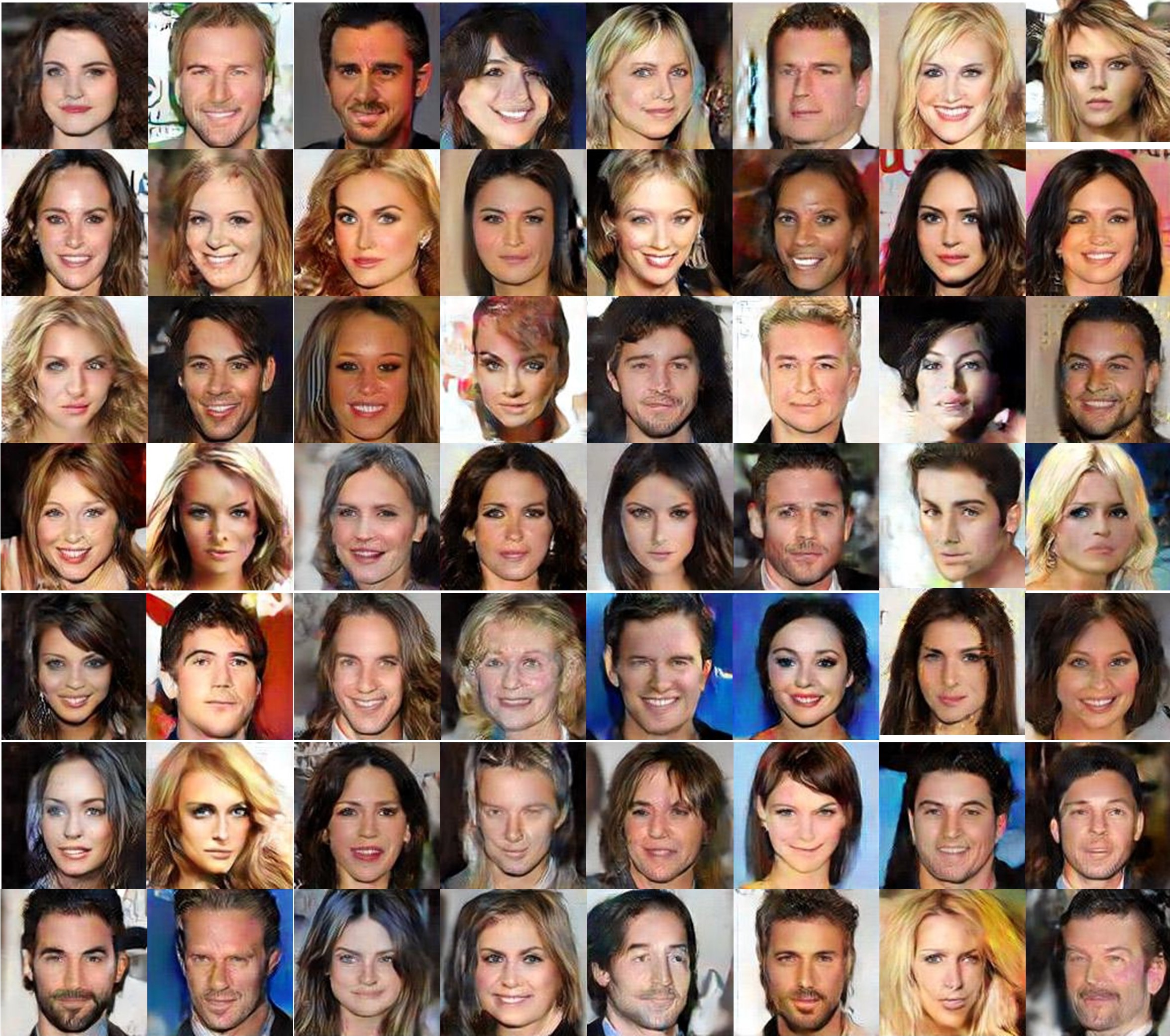
Visualization of synthesized images. The results of the experiment using Li-CFG and CFG methods can be seen in Fig. 4 and Fig. 5. Our Li-CFG method can achieve the same or better results than the CFG method. In some datasets, the image generated by the CFG method has already collapsed, while the image generated by Li-CFG still performs well. Furthermore, we also present synthesis samples generated with the state-of-the-art GAN model in CIFAR10, as shown in Fig. 6. Additional synthesis samples from various datasets can be found in Section D.4 of the supplementary materials.
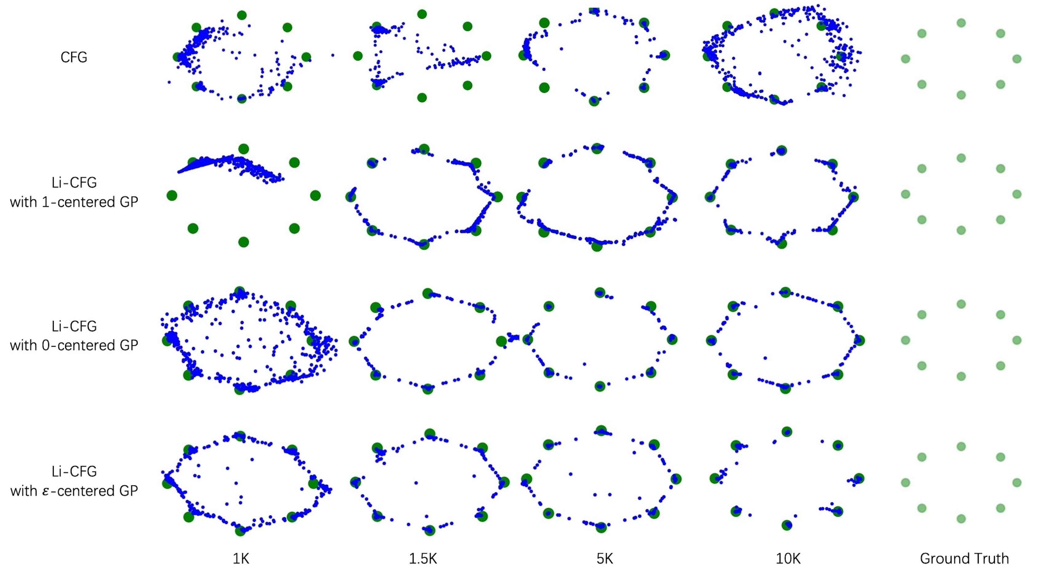
The following results were obtained for the synthetic datasets presented in Fig. 7, 8. Our observation is that the unconstrained CFG method has difficulty in converging to all modes of the ring or grid datasets. However, when supplemented with gradient penalty, these methods show an enhanced ability to converge to a mixture of Gaussians. Out of the three types of gradient penalties tested, the -centered gradient penalty showed inferior convergence compared to the -centered gradient penalty and our proposed -centered gradient penalty. Notably, our -centered gradient penalty demonstrated a higher efficacy in driving more sample points to converge to the Gaussian points compared to the -centered gradient penalty.
6 Conclusion
In this paper, We provide a novel perspective to analyze the relationship between constraint and the diversity of synthetic samples. We assert that the constraint can effectively influence the latent N-size that is strongly associated with the mode collapse phenomenon. To modify the latent N-size efficiently, we propose a new form of Gradient Penalty called -centered GP. The experiments demonstrate that our method is more stable and achieves more diverse synthetic samples compared with the CFG method. Additionally, our method can be applied not only in the CFG method but also in common GAN models. Inception score, Fréchet Distance, Precision/Recall, and visual quality of generated images show that our method is more powerful. In future work, we plan to investigate the metric function of the generator from KL diversity to the Wasserstein distance to achieve a more stable and efficient GAN architecture.
Limitations and future work. In this study, we achieve good FID results in the considered data sets. However, if given higher resolution data sets, it might lead to a different choice of our neural network architecture and hyper-parameter. On the other hand, although the hyper-parameter has an important impact on the algorithm, we do not discuss the relationship between hyper-parameter in CFG and our constraint hyper-parameter from a theoretical perspective. These effects should be systematically studied in future work.
7 Declarations
declaration - statement
-
•
Conflicts of interest/Competing interests
Not applicable
-
•
Funding
This work was funded by the National Natural Science Foundation of China U22A20102, 62272419. Natural Science Foundation of Zhejiang Province ZJNSFLZ22F020010.
-
•
Ethics approval
Not applicable
-
•
Consent to participate
Not applicable
-
•
Consent for publication
Not applicable
-
•
Availability of data and material
All the data used in our work are sourced from publicly available datasets that have been established by prior research. References for all the data are provided in our main document.
-
•
Code availability
Our code is some kind of custom code and is available for use.
-
•
Authors’ contributions
We list the Authors’ contributions as follows:
Conceptualization: [Chang Wan], [Yanwei Fu], [Xinwei Sun];
Methodology: [Chang Wan], [Xinwei Sun], [Ke Fan];
Experiments: [Chang Wan], [Ke Fan], [Yunliang Jiang];
Writing ‐ original draft preparation: [Chang Wan], [Yanwei Fu];
Writing ‐ review and editing: [Xinwei Sun], [Zhonglong Zheng], [Minglu Li];
Funding acquisition: [Yunliang Jiang], [Zhonglong Zheng];
Resources: [Zhonglong Zheng];
Supervision: [Minglu Li], [Yunliang Jiang];
All authors read and approved the final manuscript.
References
- \bibcommenthead
- Goodfellow et al. [2014] Goodfellow, I., Pouget-Abadie, J., Mirza, M., Xu, B., Warde-Farley, D., Ozair, S., Courville, A., Bengio, Y.: Generative adversarial nets. Conference on Neural Information Processing Systems 27 (2014)
- Arjovsky et al. [2017] Arjovsky, M., Chintala, S., Bottou, L.: Wasserstein generative adversarial networks. In: International Conference on Machine Learning, pp. 214–223 (2017). PMLR
- Gulrajani et al. [2017] Gulrajani, I., Ahmed, F., Arjovsky, M., Dumoulin, V., Courville, A.: Improved training of wasserstein gans. arXiv preprint arXiv:1704.00028 (2017)
- Johnson and Zhang [2018] Johnson, R., Zhang, T.: Composite functional gradient learning of generative adversarial models. In: International Conference on Machine Learning, pp. 2371–2379 (2018). PMLR
- Mescheder et al. [2018] Mescheder, L., Geiger, A., Nowozin, S.: Which training methods for gans do actually converge? In: International Conference on Machine Learning, pp. 3481–3490 (2018). PMLR
- Johnson and Zhang [2019] Johnson, R., Zhang, T.: A framework of composite functional gradient methods for generative adversarial models. IEEE Transactions on Pattern Analysis and Machine Intelligence 43(1), 17–32 (2019)
- Roth et al. [2017] Roth, K., Lucchi, A., Nowozin, S., Hofmann, T.: Stabilizing training of generative adversarial networks through regularization. arXiv preprint arXiv:1705.09367 (2017)
- Yang et al. [2019] Yang, D., Hong, S., Jang, Y., Zhao, T., Lee, H.: Diversity-sensitive conditional generative adversarial networks. arXiv preprint arXiv:1901.09024 (2019)
- Radford et al. [2015] Radford, A., Metz, L., Chintala, S.: Unsupervised representation learning with deep convolutional generative adversarial networks. arXiv preprint arXiv:1511.06434 (2015)
- Zhang et al. [2019] Zhang, H., Goodfellow, I., Metaxas, D., Odena, A.: Self-attention generative adversarial networks. In: International Conference on Machine Learning, pp. 7354–7363 (2019). PMLR
- Karras et al. [2017] Karras, T., Aila, T., Laine, S., Lehtinen, J.: Progressive growing of gans for improved quality, stability, and variation. arXiv preprint arXiv:1710.10196 (2017)
- Brock et al. [2018] Brock, A., Donahue, J., Simonyan, K.: Large scale gan training for high fidelity natural image synthesis. arXiv preprint arXiv:1809.11096 (2018)
- Karras et al. [2019] Karras, T., Laine, S., Aila, T.: A style-based generator architecture for generative adversarial networks. In: IEEE/CVF Computer Vision and Pattern Recognition Conference, pp. 4401–4410 (2019)
- Che et al. [2016] Che, T., Li, Y., Jacob, A.P., Bengio, Y., Li, W.: Mode regularized generative adversarial networks. arXiv preprint arXiv:1612.02136 (2016)
- Nowozin et al. [2016] Nowozin, S., Cseke, B., Tomioka, R.: f-gan: Training generative neural samplers using variational divergence minimization. In: Conference on Neural Information Processing Systems, pp. 271–279 (2016)
- Nagarajan and Kolter [2017] Nagarajan, V., Kolter, J.Z.: Gradient descent gan optimization is locally stable. arXiv preprint arXiv:1706.04156 (2017)
- Mescheder et al. [2017] Mescheder, L., Nowozin, S., Geiger, A.: The numerics of gans. arXiv preprint arXiv:1705.10461 (2017)
- Oberman and Calder [2018] Oberman, A.M., Calder, J.: Lipschitz regularized deep neural networks converge and generalize. arXiv preprint arXiv:1808.09540 (2018)
- Scaman and Virmaux [2018] Scaman, K., Virmaux, A.: Lipschitz regularity of deep neural networks: analysis and efficient estimation. arXiv preprint arXiv:1805.10965 (2018)
- Zhou et al. [2018] Zhou, Z., Song, Y., Yu, L., Wang, H., Liang, J., Zhang, W., Zhang, Z., Yu, Y.: Understanding the effectiveness of lipschitz-continuity in generative adversarial nets. arXiv preprint arXiv:1807.00751 (2018)
- Zhou et al. [2019] Zhou, Z., Liang, J., Song, Y., Yu, L., Wang, H., Zhang, W., Yu, Y., Zhang, Z.: Lipschitz generative adversarial nets. In: International Conference on Machine Learning, pp. 7584–7593 (2019). PMLR
- Herrera et al. [2020] Herrera, C., Krach, F., Teichmann, J.: Estimating full lipschitz constants of deep neural networks. arXiv preprint arXiv:2004.13135 (2020)
- Kim et al. [2021] Kim, H., Papamakarios, G., Mnih, A.: The lipschitz constant of self-attention. In: International Conference on Machine Learning, pp. 5562–5571 (2021). PMLR
- Miyato et al. [2018] Miyato, T., Kataoka, T., Koyama, M., Yoshida, Y.: Spectral normalization for generative adversarial networks. arXiv preprint arXiv:1802.05957 (2018)
- Bhaskara et al. [2022] Bhaskara, V.S., Aumentado-Armstrong, T., Jepson, A.D., Levinshtein, A.: Gran-gan: Piecewise gradient normalization for generative adversarial networks. In: Proceedings of the IEEE/CVF Winter Conference on Applications of Computer Vision, pp. 3821–3830 (2022)
- Wu et al. [2021] Wu, Y.-L., Shuai, H.-H., Tam, Z.-R., Chiu, H.-Y.: Gradient normalization for generative adversarial networks. In: InternationalConference on Computer Vision, pp. 6373–6382 (2021)
- Li et al. [2022] Li, Y., Mo, Y., Shi, L., Yan, J.: Improving generative adversarial networks via adversarial learning in latent space. Conference on Neural Information Processing Systems 35, 8868–8881 (2022)
- Mao et al. [2019] Mao, Q., Lee, H.-Y., Tseng, H.-Y., Ma, S., Yang, M.-H.: Mode seeking generative adversarial networks for diverse image synthesis. In: IEEE/CVF Computer Vision and Pattern Recognition Conference, pp. 1429–1437 (2019)
- Metz et al. [2016] Metz, L., Poole, B., Pfau, D., Sohl-Dickstein, J.: Unrolled generative adversarial networks. arXiv preprint arXiv:1611.02163 (2016)
- Li et al. [2021] Li, Y., Shi, L., Yan, J.: Iid-gan: an iid sampling perspective for regularizing mode collapse. arXiv preprint arXiv:2106.00563 (2021)
- LeCun et al. [1998] LeCun, Y., Bottou, L., Bengio, Y., Haffner, P.: Gradient-based learning applied to document recognition. Proceedings of the IEEE 86(11), 2278–2324 (1998)
- Krizhevsky et al. [2009] Krizhevsky, A., Hinton, G., et al.: Learning multiple layers of features from tiny images. Master’s thesis, Department of Computer Science, University of Toronto (2009)
- Yu et al. [2015] Yu, F., Seff, A., Zhang, Y., Song, S., Funkhouser, T., Xiao, J.: Lsun: Construction of a large-scale image dataset using deep learning with humans in the loop. arXiv preprint arXiv:1506.03365 (2015)
- Deng et al. [2009] Deng, J., Dong, W., Socher, R., Li, L.-J., Li, K., Fei-Fei, L.: Imagenet: A large-scale hierarchical image database. In: IEEE/CVF Computer Vision and Pattern Recognition Conference, pp. 248–255 (2009). Ieee
- Mao et al. [2017] Mao, X., Li, Q., Xie, H., Lau, R.Y., Wang, Z., Paul Smolley, S.: Least squares generative adversarial networks. In: InternationalConference on Computer Vision, pp. 2794–2802 (2017)
- Lim and Ye [2017] Lim, J.H., Ye, J.C.: Geometric gan. arXiv preprint arXiv:1705.02894 (2017)
- He et al. [2016] He, K., Zhang, X., Ren, S., Sun, J.: Deep residual learning for image recognition. In: IEEE/CVF Computer Vision and Pattern Recognition Conference, pp. 770–778 (2016)
- Xiao et al. [2021] Xiao, Z., Kreis, K., Vahdat, A.: Tackling the generative learning trilemma with denoising diffusion gans. arXiv preprint arXiv:2112.07804 (2021)
- Salimans et al. [2016] Salimans, T., Goodfellow, I., Zaremba, W., Cheung, V., Radford, A., Chen, X.: Improved techniques for training gans. Conference on Neural Information Processing Systems 29, 2234–2242 (2016)
- Heusel et al. [2017] Heusel, M., Ramsauer, H., Unterthiner, T., Nessler, B., Hochreiter, S.: Gans trained by a two time-scale update rule converge to a local nash equilibrium. Conference on Neural Information Processing Systems 30 (2017)
- Kynkäänniemi et al. [2019] Kynkäänniemi, T., Karras, T., Laine, S., Lehtinen, J., Aila, T.: Improved precision and recall metric for assessing generative models. Conference on Neural Information Processing Systems 32 (2019)
- Zadorozhnyy et al. [2021] Zadorozhnyy, V., Cheng, Q., Ye, Q.: Adaptive weighted discriminator for training generative adversarial networks. In: IEEE/CVF Computer Vision and Pattern Recognition Conference, pp. 4781–4790 (2021)
Appendix
Appendix A Overview
In this section, we outline the contents of our supplementary material, which is divided into four main sections. Firstly, we introduce the supplementary material. Secondly, we delve into the analysis of the dynamic theory for the CFG method. This section covers essential concepts related to CFG, the Lipschitz constraint, and the analysis of the dynamic theory of CFG. Thirdly, the theoretical analysis of our theory section contains the proof of our definition, Lemma and Theorem. Finally, we showcase the results of our experiments in the last section.
In the analysis of dynamic theory for the CFG method section, we provide foundational knowledge about CFG and Lipschitz constraints. Furthermore, we provide theoretical proofs that establish certain equivalences between the CFG method and conventional GAN theory, specifically focusing on dynamic theory principles.
In the theoretical analysis of our theory section, we initiate our exploration by presenting the proofs for both Definition 3.1 and the Proposition 3.5. The Definition 3.1 is a base definition for Proposition 3.5, so we prove them together. The Proposition 3.5 gives the formulation for the latent N-size with gradient penalty. Moving forward, we provide the proof of the corollary that , which is an important corollary that deviates our -centered gradient penalty. Subsequently, we provide the proof of the Lemma 3.6 which deviates the relationship between the value of the discriminator norm under three different gradient penalties. Lastly, we provide the proof of our main Theorem 3.7 which summarizes the relationship between the latent N-size and three gradient penalties under the above definitions and Lemmas.
In the Experiments section, we provide additional experiments and present more results of our Li-CFG and -centered method with common GAN models. When working with synthetic datasets, we include visual inspection figures compared our -centered method to other GAN models that use different gradient penalties. In our work with real-world datasets, we will create visual comparison figures to evaluate the performance of the CFG method and Li-CFG on different databases, including CeleBA, LSUN Bedroom, and ImageNet. We will compare these methods at resolutions of 128x128 and 256x256 pixels. Moreover, we’ll also present visual comparison figures of our -centered method with DDGAN and BigGAN in LSUN Church (256x256) and ImageNet (64x64).
Appendix B Analysis of the dynamic theory for the CFG
Dynamic Theory for the CFG. This section encompasses the motivation behind and proofs for the relationship between the CFG method and the common GAN method. In terms of the dynamic theory, the generator and discriminator in the CFG method function equivalently to the corresponding components in common GAN. Based on this analysis, the CFG method still surfers unstable and not locally convergent problems at the Nash-equilibrium point. We visualize the gradient vector of the discriminator for CFG and Li-CFG in Fig. 9. This serves as the impetus for us to introduce the Lipschitz constraint to the CFG method, aiming to enforce convergence. The dynamic theory is imported from Mescheder et al. [5] and Nagarajan and Kolter [16].

Lemma B.1.
The loss functions of the discriminators of CFG and common GAN learned by minimax games exhibit the same form and optimization objective. The form of the discriminator loss function is:
Proof.
We can establish the equivalence through two main perspectives. Firstly, we analyze the CFG method. The loss function of the discriminator can be described as follows:
| (11) |
To unify the symbolic expression, we use instead of from the CFG article in our paper. The common GAN loss function is
| (12) |
If we set the and substitute it into the common GAN loss function, we can get the Loss function of the CFG method. This demonstrates the equivalence between the two loss functions. From the second part, we can use the notation of the loss function proposed by Nagarajan and Kolter [16] to prove the lemma. The loss function is
| (13) |
If we choose the f function to be , it leads to the loss function of the CFG method. ∎
We demonstrate the process with more detailed proof. First, we list the loss functions of the three discriminators for comparison. The discriminator’s loss function proposed by Nagarajan and Kolter [16] is
| (14) |
But in the notation of Mescheder et al. [5], the loss function is
| (15) |
We think both the equation are correct, and choose the Eq. (14) in our proof process. As for simplification, we omit the symbol . Furthermore, we use the symbols and to denote the discriminator and generator, respectively. The loss function of the discriminator of the CFG method is
| (16) |
The discriminator loss function of common GAN is
| (17) |
Our goal is to prove that the three loss functions are equivalent. One loss function can be transformed into others under certain conditions.
We set the and substitute it into the Eq. (17). Then we have
The equation in the bracket is the loss function of the CFG method. has the same optimization objectives as the . So both loss functions are equivalent. It is easy to transform the Eq. (16) to Eq. (17) as we set the .
We choice the f function to be . The equation is similar to the if we substitute the into Eq. (14), it leads to the loss function of CFG method. Both equations are equivalent. So the Lemma B.1 is proved.
Lemma B.2.
The gradient vector field of generators of CFG and common GAN learned by minimax games exhibit the same form in the dynamic theory. The form of the gradient vector field is:
We want to prove that . denotes the gradient vector field of the common GAN generator, while represents the generator gradient vector field of the CFG method. denotes the weight vector of the generator instead of . If the two gradient vector fields are equal to each other, we can say that proof of Lemma B.2 is done.
Proof.
we expand the , the gradient vector field of generator for common GAN
| (18) |
The value of is . We substitute the into , then
| (19) |
We extract the out and derive it as follows:
| (20) |
We bring it back into the , we will get
| (21) |
This is the gradient vector field of common GAN.
Now we check the gradient vector field of the CFG method. For the CFG method, a hyper-parameter has been used to control the varying steps of generators
| (22) |
The variables and have the same meaning. we will discuss the M in two cases to analyze the gradient vector field of the generator for the CFG method. The loss function of the generator for the CFG method is
| (23) |
First, when we consider =1. In this case, the loss function can be written as
| (24) |
. Then the gradient vector field can be written as below:
| (25) |
For , we archive the above result. Now we compare the form of and . If we set the = , the two function are both scaling factor. We find two equations get exactly the same form. So the proof is done.
Next, When we consider the second case, and . The expansion of Eq. (22) can be written as below:
| (26) |
Let us sum the right side of the equation list, and we get the form of by as:
| (27) |
Now we consider the . When , the gradient vector field can be written as
| (28) |
So we get the gradient vector field of the CFG method when . Every sub-item in the equation is a gradient vector that has the same form as the gradient vector when , which is equivalent to common GAN. The Sum of these gradient vectors is CFG method which is also equivalent to common GAN. So Lemma 3.2 is proved. ∎
Appendix C Theoretical analysis of our theory
C.1 Latent N-size with gradient penalty
In this section, we will provide a detailed proof procedure for Definition 3.1 and Proposition 3.5. Since Definition 3.1 is the foundational definition for Proposition 3.5, the detailed proof procedure for Definition 3.1 will be presented in the proof of Proposition 3.5.
Latent N-size. We illustrate the concept of latent N-size, which serves as the foundational definition for the subsequent theory.
Definition 3.1.
Let , be two samples in the latent space. Suppose is attracted to the mode by , then there exists a neighborhood of such that is distracted to by , for all . The size of can be arbitrarily large but is bounded by an open ball of radius . The is defined as
According to this definition, the radius is inversely proportional to the discrepancy between the preceding and subsequent outputs of the generator, given a similar latent vector . A large value of results in a small difference between the previous and subsequent generator outputs, leading to mode collapse. Conversely, a small value of leads to a large difference, resulting in diverse synthesis.
Latent N-size and the diversity. We offer three fundamental definitions of the latent N-size and demonstrate its relationship to the diversity of synthetic samples.
Definition 3.2 (Modes in Image Space).
There exist some modes cover the image space . Mode is a subset of satisfying and , where and belong to the same mode , and belong to different modes , and .
Definition 3.3 (Modes Attracted).
Let be a sample in latent space, we say is attracted to a mode by from a gradient step if , where is an image in a mode , denotes a small quantity, and are the generator parameters before and after the gradient updates respectively.
Definition 3.4 (Modes Distracted).
Let be a sample in latent space, we say is distracted to a mode by from a gradient step if , where is an image in a mode , is an image from other modes, keeps the same meaning as in Definition 3.2, and are the generator parameters before and after the gradient updates respectively.
Latent N-size with gradient penalty. We demonstrate the relationship between the latent N-size and the gradient penalty. According to Proposition 3.5, as increases, the latent N-size decreases, and vice versa.
Proposition 3.5.
can be defined with discriminator gradient penalty as follows:
, where and . stands for the discriminator gradient penalty.
C.2 -centered GP
Observe from Eq. (3) and Eq. (4) in CFG method, we can derive the following conclusion: . This is an important corollary derived from the CFG method. With this corollary, we can prove that the latent N-size corresponding to our -centered GP is the smallest among all three gradient penalties in the following section.
Proof.
The Eq. (3) from CFG implies that for to be negative so that the distance decreases, we should choose to be:
where is an arbitrary scaling factor. is a vector function such that and that if and only if , e.g., or . With this choice of , we obtain
that is, the distance is guaranteed to decrease unless the equality holds. So, we can know that . Then, we scrutiny the Eq. (4) from which can deviate the equation:
where is an arbitrary scaling factor, , , when is KL-divergence and when , which is the analytic solution of the CFG discriminator. Based on the above formulation, we can find that is a scaling function that is always greater than 0, is a exponential function, and is a non negative function composed of exponential function . So if equation holds, the also holds. ∎
We define our method as the -centered Gradient Penalty. We use notation in our penalty name and equation to differ from the hyper-parameter . The -centered GP is
| (33) |
where is a vector such that with , and are dimensions and channels of the real data respectively. is sampled uniformly on the line segment between two random points vector .
Combining the corollary , our -centered GP increases the as to achieve a better latent N-size which other two gradient penalty behaviors worse.
C.3 Latent N-size with different gradient penalty
In this section, we will derive our final theorem about the latent N-size with different gradient penalties.
First, we establish the relationship among the latent N-size for three gradient penalties in the following Lemma. We will substitute different types of gradient penalty into the Proposition 3.5.
Lemma 3.6.
The norms of the three Gradient Penalties, which dictate the latent N-size, are defined as follows: = , , =, respectively. The order of magnitude between the norms of three Gradient Penalty is . Consequently, the relationship between the latent N-size of three Gradient Penalty is .
Proof.
Let us start with the result from the Eq .32. We will insert three distinct Gradient Penalties into it and determine the latent N-size for each of these penalties. Next, we will focus on the primary component of the three equations and compare the values among them.
The equation of the -centered gradient penalty is
| (34) |
The equation of -centered gradient penalty is
| (35) |
The equation of -centered gradient penalty is
| (36) |
We bring them back to the Eq .(29) and expand the Gradient Penalty expression. We omit the expectation symbol and focus on the gradient. Then, we plug the above results into Eq .32 and we have the different gradient penalty equation for the sum of the additions in latent N-size parentheses. As for simplicity, we just focus on it and omit other symbols. We called it the determined part of the latent N-size.
The determined part of the latent N-size of -centered gradient penalty is
| (37) |
The determined part of the latent N-size of -centered gradient penalty is
| (38) |
With prior knowledge from CFG that , The determined part of the latent N-size of -centered gradient penalty is
| (39) |
For the square items in Eq. (37), Eq. (LABEL:dpgp0), Eq. (LABEL:dpgp2), we show that the
| (40) |
Based on this conclusion, we can observe that the relationship among the latent N-size with different gradient penalties is as follows: . ∎
Theorem 3.7.
Suppose is attracted to the mode by , then there exists a neighborhood of such that is distracted to by , for all . The size of can be arbitrarily large but is bounded by an open ball of radius where be controlled by Gradient Penalty terms of the discriminator. The relationship between the radius’s size of three Gradient Penalty is .
Proof.
This theorem encompasses three key implications. Firstly, when the latent vector is attracted to a mode within the image space, the corresponding latent N-size should not be overly large, which can be attributed to two distinct reasons. One, vectors within the neighborhood are more likely to be attracted to the same mode. Two, vectors within this neighborhood face challenges in being attracted to other modes within the image space, with the level of difficulty determined by an upper bound expressed as . This bound is constructed based on the distances between different modes and within the same mode within the image space.
Secondly, the discriminator gradient penalty in the CFG formulation can regulate the latent N-size. This introduces a trade-off between diversity and training stability. For instance, the -centered gradient penalty ensures stable and convergent training near the Nash equilibrium, but it leads to a minimal discriminator norm, resulting in a larger latent N-size and reduced diversity.
Thirdly, by augmenting the norm of the discriminator, our -centered gradient penalty achieves the smallest latent N-size, consequently leading to the highest level of diversity.
Appendix D Experiments
In this section, we describe additional experiments and give a more visual representation. In addition to the databases mentioned in the paper, we also conducted training on the CeleBA and LSUN Bedroom datasets with resolutions of 128x128 and 256x256. We will provide visual inspections and results for these additional databases.
D.1 Hyper-parameter
In the practice stage, the is a -value constant vector which has the same dimension of . The dimension of is [C, H, W], the flatten of dimension equals . Our image data has the pixels height, pixels weight, and channels. The will be written as . is the symbol of norm 2. So the value of can be written as
| (41) |
where , . The is a hyper-parameter that controls the tight bound of . We will set in the ablation study to show the effeteness. It is easy to understand the because this is a small enhancement of the discriminator norm and thus to a smaller latent N-size. If we set the , the varying range of is too large which leads to a too-small latent N-size, thus leads to a non-convergent result for the neural network. The loss function of the training process will not converge and the synthetic samples will transform to noise. We present the ablation result in Table. 8 and Table. 7
| FID | IS | |||||||
|---|---|---|---|---|---|---|---|---|
| MNIST | ||||||||
| ours(-centered) | 2.99 | 2.88 | 2.85 | untrained | 2.28 | 2.32 | 2.29 | untrained |
| -centered | 3.54 | 3.54 | 3.54 | 3.54 | 2.31 | 2.31 | 2.31 | 2.31 |
| -centered | 3.64 | 3.64 | 3.64 | 3.64 | 2.3 | 2.3 | 2.3 | 2.3 |
| FID | IS | |||||||
|---|---|---|---|---|---|---|---|---|
| LSUN Bedroom | ||||||||
| ours(-centered) | 9.94 | 8.78 | 9.73 | untrained | 2.97 | 2.94 | 2.97 | untrained |
| -centered | 10.54 | 10.54 | 10.54 | 10.54 | 3.067 | 3.067 | 3.067 | 3.067 |
| -centered | 11.5 | 11.5 | 11.5 | 11.5 | 3.154 | 3.154 | 3.154 | 3.154 |
| FID | IS | |||||||
| LSUN T (=1) | ||||||||
| ours(-centered) | 11.41 | 19.47 | 21.59 | 4.6 | 4.5 | 4.42 | ||
| -centered | 12.33 | 19.94 | 21.71 | 4.57 | 4.6 | 4.53 | ||
| -centered | 12.81 | 22.17 | 22.71 | 4.47 | 4.46 | 4.5 | ||
| CFG method | 13.54 | 13.54 | 13.54 | 4.38 | 4.38 | 4.38 | ||
| LSUN T (=5) | ||||||||
| ours(-centered) | 19.18 | 21.58 | 21.69 | 4.48 | 4.49 | 4.34 | ||
| -centered | 20.29 | 24.77 | 23.02 | 4.47 | 4.43 | 4.43 | ||
| -centered | 24.09 | 29.39 | untrained | 4.37 | 4.41 | untrained | ||
| CFG method | 22.3 | 22.3 | 22.3 | 4.34 | 4.34 | 4.34 | ||
| LSUN T (=10) | ||||||||
| ours(-centered) | 21.3 | 23 | 20.7 | 4.43 | 4.42 | 4.53 | ||
| -centered | 23.68 | 19.74 | 20.7 | 4.39 | 4.46 | 4.38 | ||
| -centered | 23.49 | untrained | untrained | 4.3 | untrained | untrained | ||
| CFG method | 25.53 | 25.53 | 25.53 | 4.2 | 4.2 | 4.2 | ||
If our experiment setting does not satisfy these conditions, the synthetic samples make noise or collapse. We show the visual inspection of different settings for MNIST and LSUN Bedroom in Fig. 10 and Fig. 11.


| FID | IS | ||||||
|---|---|---|---|---|---|---|---|
| LSUN T+B | |||||||
| ours(-centered) | 15.72 | 16.85 | 16.67 | 5.07 | 5.06 | 5.08 | |
| -centered | 16.01 | 17.4 | 19.79 | 5.05 | 5.08 | 5.05 | |
| -centered | 16.32 | 18.73 | 34.28 | 5.04 | 5.18 | 4.71 | |
D.2 Effect of with different penalty
In most cases, a gradient penalty with a center within a small interval around 0 tends to yield better results. However, on some datasets, a gradient penalty centered around 1 might perform better. Our method provides a controllable parameter that allows the center of the gradient penalty to vary within the range specified by the parameter, and we experimentally show that our method yields better results. For the parameters where the CFG method performs well, using a value of 0.1 for the parameter consistently yields improved results. Conversely, for those parameter settings of where the CFG method shows poor or inadequate training performance, using a value of 10 for the parameter often leads to better overall performance. We compare the results of different values for CFG and Li-CFG in Table. 9 and Table. 10.
D.3 Effect of Gradient Penalty with different
The results of the CFG method can exhibit significant variations in response to minor changes in parameter values. This phenomenon is illustrated in Fig. 12, where we observe that different choices of the parameter lead to diverse outcomes. However, by introducing the gradient penalty, the CFG method consistently demonstrates increased stability across various values. Notably, in cases where the CFG method struggles to converge, the addition of the gradient penalty leads to improved results.

D.4 Visual inspection of synthesized images
In this section, we introduce the visual inspection figures of the CFG method, Li-CFG, and other GAN models. The Fig. 27, 28, 29, 32, 30, 31, 33 are separated into two columns of real images and generated images respectively. The real images are represented in the left column while the generated images are displayed in the right column which contains different GP regularization with Li-CFG. The settings of generated images in the CFG method and Li-CFG are almost the same. We also display the generated images with CeleBA, LSUN Bedroom and ImageNet with resolution of 128 and 256. We present the results of synthetic datasets in the Fig. 13, 14, 15, 16, 17, 18, 19, 20. Moreover, we showcase the results of BigGAN and DDGAN from real-world datasets in the Fig. 21, 22, 23.


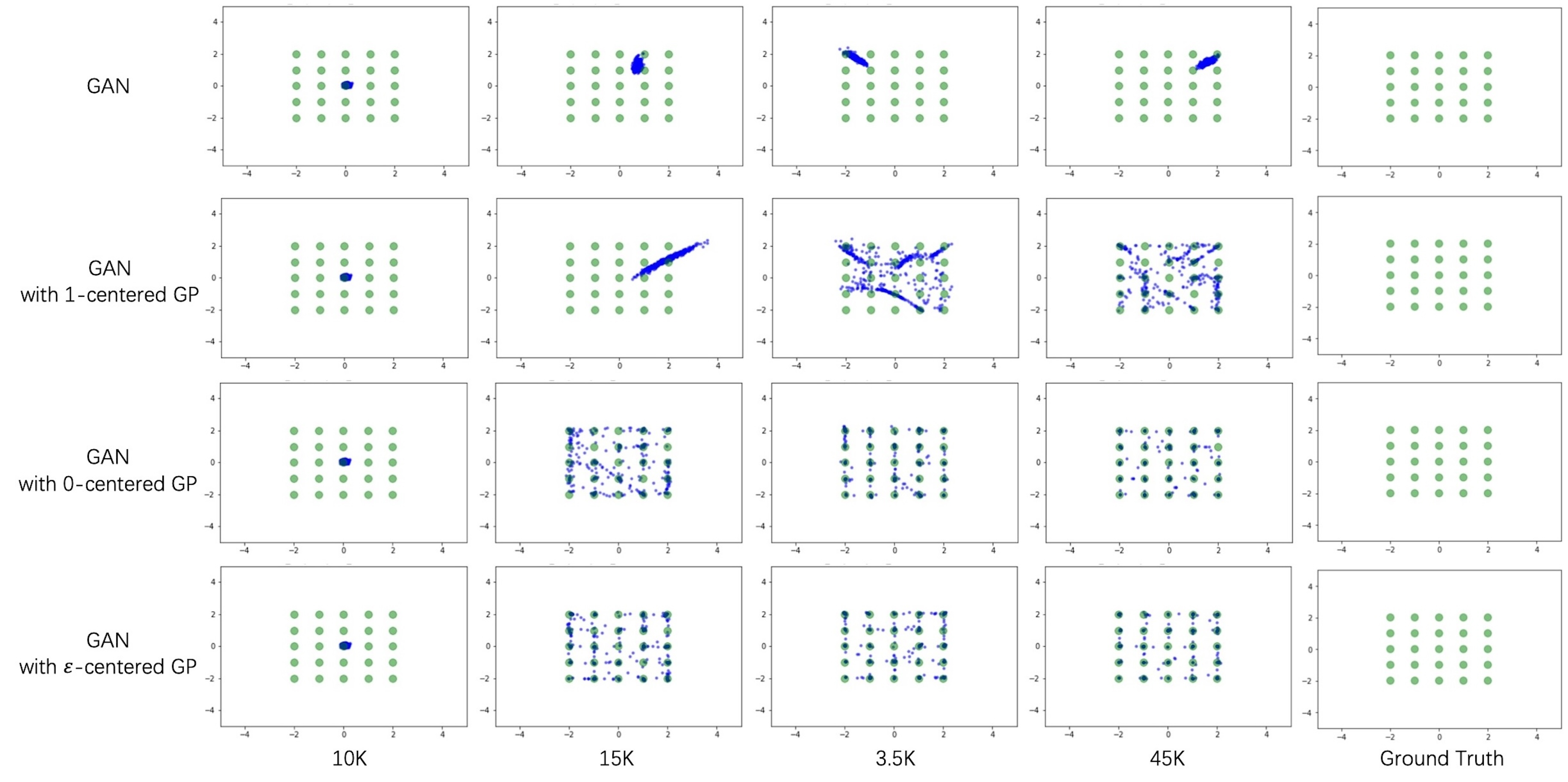


Synthetic Datasets. In the present results from synthetic datasets, we observed that unconstrained methods like the original GAN, LSGAN, WGAN and HingeGAN struggle to converge to all modes of the ring or grid datasets. However, these methods, when supplemented with gradient penalty, show an enhanced ability to converge to a mixture of Gaussians. Among the three types of gradient penalties tested, the -centered gradient penalty exhibited inferior convergence compared to the -centered gradient penalty and our proposed -centered gradient penalty. Notably, our -centered gradient penalty demonstrated a higher efficacy in driving more sample points to converge to the Gaussian points compared to the -centered gradient penalty.
ImageNet. We present the experiment results of Li-CFG on the ImageNet datasets here. We compare the FID result of Li-CFG and CFG methods which are the same Neural architecture with parameters of different magnitudes. The Neural architecture simply uses the DCGAN and the res-block. Fig. 24 shows the FID scores of the CFG method, the CFG method with two times the number of parameters, and Li-CFG with twice the number of parameters. Fig. 25 presents the visualization effect of the above three models. Fig. 26 manifest our Li-CFG results on the ImageNet datasets.