A New Class of Compact Formulations for Vehicle Routing Problems
Abstract
This paper introduces a novel compact mixed integer linear programming (MILP) formulation and a discretization discovery-based solution approach for the Vehicle Routing Problem with Time Windows (VRPTW). We aim to solve the optimization problem efficiently by constraining the linear programming (LP) solutions to use only flows corresponding to time and capacity-feasible routes that are locally elementary (prohibiting cycles of customers localized in space).
We employ a discretization discovery algorithm to refine the LP relaxation iteratively. This iterative process alternates between two steps: (1) increasing time/capacity/elementarity enforcement to increase the LP objective, albeit at the expense of increased complexity (more variables and constraints), and (2) decreasing enforcement without decreasing the LP objective to reduce complexity. This iterative approach ensures we produce an LP relaxation that closely approximates the optimal MILP objective with minimal complexity, facilitating an efficient solution via an off-the-shelf MILP solver.
The effectiveness of our method is demonstrated through empirical evaluations on classical VRPTW instances. We showcase the efficiency of solving the final MILP and multiple iterations of LP relaxations, highlighting the decreased integrality gap of the final LP relaxation. We believe that our approach holds promise for addressing a wide range of routing problems within and beyond the VRPTW domain.
1 Introduction
This paper proposes a novel compact formulation for the Vehicle Routing Problem with Time Windows (VRPTW) with an empirically “tighter” linear programming (LP) relaxation compared to a standard two-index compact formulation baseline, which can be solved directly as a Mixed Integer Linear Program (MILP). By “tighter,” we mean that the LP relaxation’s optimal solution objective value is closer to the MILP objective value relative to a baseline LP. We characterize such a formulation with two properties: sufficiency and parsimony. Sufficiency indicates that our formulation describes the tightest LP within a considered class of LPs, while parsimony ensures that our formulation is as compact as possible (measured by the number of variables and constraints) without decreasing the LP objective. Utilizing these properties, we devise an algorithm that iteratively expands and contracts this formulation and demonstrates its monotonic convergence to a solution that is both sufficient and parsimonious. By producing a sufficient and parsimonious MILP we aim to ensure that the MILP can be solved efficiently. Moreover, adjusting the formulation parameters allows us to explore the trade-off between solution time and quality.
Our approach augments the standard compact formulation by enforcing agreement between the standard compact decision variables and separate sets of variables and constraints designed to enforce elementarity, time feasibility, and capacity feasibility. Agreement between these formulations and the compact formulation requires that the number of edges indicating travel from one location to another agrees with the original compact variables. Restrictions on time and capacity feasibility are enforced using discretization of time/capacity ranges into “buckets” , inspired by previous work (Boland et al., 2017, 2019), while restrictions on elementarity use Local Area Arcs from our recent work (Mandal et al., 2023, 2022). We elaborate on our use of these enforcement mechanisms below.
Restricting Violations of Capacity/Time Feasibility: We partition the remaining capacity before servicing each customer into “buckets”, creating nodes for a directed acyclic graph. Each pair of nodes corresponding to feasible flow is connected and associated with a decision variable. A valid solution associated with this directed acyclic graph is a weighted non-negative sum of source-to-sink paths. Operations aiming towards sufficiency reduce the granularity of the partitions. Operations aiming towards parsimony increase the granularity without decreasing the LP objective. This approach is used for time-enforcing temporal feasibility as well.
Restricting Violations of Elementarity: For each customer, we create variables representing all possible immediately succeeding sequences of nearby customers. These sequences are limited to those that can be used in an optimal solution, given the intermediate customers, those on the efficient frontier of minimal cost, earliest completion time, and latest start time. We require one variable to be selected for each customer. Operations aiming toward sufficiency expand the set of nearby customers and, hence, the number of variables. This limits the set of cycles of customers allowed, at the cost of increasing the complexity of the LP. Operations aiming towards parsimony analyze the dual solution to decrease the set of nearby customers, decreasing the complexity of the LP in such a manner as not to decrease the LP objective. We should note that the use LA-arcs for cycle elimination, enables users to expand their formulation’s scale as MILP solvers’ computational capabilities advance.
We organize this document as follows. Section 2 briefly reviews the most relevant literature. Section 3 presents the VRPTW and its compact two-index formulation. Section 4 provides the proposed LP relaxation for the VRPTW. Section 5 provides an algorithm called LA-Discretization to solve the corresponding relaxation efficiently. Section 6 we consider LA-Arc generation in detail. Section 7 provides experimental results comparing LA-Discretization to a baseline compact two-index formulation. Section 8 provides conclusions and discusses extensions.
2 Literature Review
Different MILP formulations for VRPTW trade off the increase in the number of variables/constraints against the tightness of the LP relaxation. The use of a tighter formulation often means that branch & bound expands fewer nodes; however, this tightness often comes at the cost of a larger LP (in terms of more variables/constraints), which is thus more computationally intensive to solve at each node of the branch & bound solver. Well-known expanded or Dantzig-Wolfe formulations (Dantzig and Wolfe, 1960) often provide much tighter linear programming (LP) relaxations than a standard compact formulation for MILPs in many application areas (Barnhart et al., 1996; Geoffrion, 1974). These formulations are solved through Column Generation (CG) (Gilmore and Gomory, 1961) and are widely used across many problem domains, including vehicle routing (Desrochers et al., 1992), crew scheduling (Desaulniers et al., 1997), and more recently applications in artificial intelligence domains, such as computer vision (Yarkony et al., 2020) and machine learning (Lokhande et al., 2020).
Expanded formulations used to solve Vehicle Routing Problems (VRP) are weighted set covering formulations where each column (primal variable) corresponds to a feasible route, and each cover constraint (primal constraint) corresponds to a customer, which must be serviced. The expanded formulation circumvents multiple key difficulties of a compact formulation, the most important of which is the following. The expanded formulation enforces that the flows of the corresponding compact formulation only describe feasible routes. However, expanded formulations present multiple difficulties including the following.
-
•
When the LP solution includes fractional variables at the termination of CG, the set of columns (variables in the MILP) generated over the course of CG does not necessarily include all columns that are part of the optimal integer solution. Thus, we cannot use a standard off-the-shelf MILP solver to guarantee an optimal solution. The importance of this difficulty is emphasized in (Barnhart et al., 1996), which observes that columns that describe an optimal solution to the weighted set cover LP may not express an optimal or even a near-optimal solution to the weighted set cover integer linear program (ILP). Branch & Price (Barnhart et al., 1996) or Branch-Cut & Price (Gauvin et al., 2014; Pecin et al., 2017) can be used to solve these formulations to optimality, but are difficult to implement.
-
•
Generating negative (or positive in the case of a maximization objective) reduced cost columns is often a challenging optimization problem. In the context of VRPs, these boil down to an elementary resource-constrained shortest path problem (Irnich and Desaulniers, 2005) (ERCSPP), which is NP-hard. ERCSPP solvers are tricky to implement, which has led researchers to propose numerous sophisticated implementations in the last decades (Righini and Salani, 2008, 2009; Baldacci et al., 2011; Boland et al., 2006; Righini and Salani, 2006; Lozano et al., 2016; Tilk et al., 2017; Beasley and Christofides, 1989; Righini and Salani, 2004; Cabrera et al., 2020; Lozano and Medaglia, 2013; Li and Han, 2019).
-
•
Valid inequalities such as subset-row inequalities (Jepsen et al., 2008) or rounded capacity inequalities (Archetti et al., 2011) must be separated by the CG developer, and these may alter the structure of the CG pricing problem (as is the case for (Jepsen et al., 2008)), which can add further complexity to the pricing problem as additional resources must be included in ERCSPP.
- •
Elementarity, the property that a customer may be present at most once in a route, can be very challenging to enforce in pricing. The following approaches attempt to avoid fully/explicitly considering elementarity in routes in pricing problems in CG formulations: neighborhood (NG)-route relaxations (Baldacci et al., 2011, 2012), decremental state space relaxations (DSSR) (Righini and Salani, 2009), P-step formulations (Dollevoet et al., 2020), Q-route relaxations (Christofides et al., 1981) and Local Area (LA)-route relaxations (Mandal et al., 2022, 2023). In NG-route relaxations (Baldacci et al., 2012), the elementarity of the route is relaxed only to prevent cycles of customers localized in space. Specifically, when extending a label during pricing, we hold onto customers from the previous label that are in the NG-neighborhood (nearby customers) of the latest customer at the given label. We forbid the extension of a label to a customer where the label states that it has already been. DSSR can be understood as expanding the NG-neighborhood as needed (Righini and Salani, 2008, 2009), hence, gradually enforcing elementarity where violated. Q-route relaxations relax elementarity to prevent cycles that contain any sub-sequence in which a customer is preceded and succeeded by the same customer. P-step formulations (Dollevoet et al., 2020) employ an arc-based formulation where arcs correspond to elementary sequences of customers. CG is employed to solve optimization since the number of such sequences can be quite large. LA-routes (Mandal et al., 2022) construct routes as sequences of elementary sub-sequences of customers where each sub-sequence is localized in space.
The work of (Boland et al., 2017) with respect to continuous-time service network design problems can be used to enforce feasibility with regard to time in VRPTWs. In that paper, the authors intelligently construct a partition of the times in a time-expanded graph representation of the underlying problem. This partition induces a relaxation of time feasibility. Specifically, a vehicle can depart at any time in an interval, given that it arrives at any time in that interval. The weakness is that this partition permits a vehicle to leave a node before it arrives. No relaxation occurs if the partition is constructed such that arrivals at nodes only occur at the earliest time possible in the optimal solution. To construct such a partition, the authors iterate between solving the MILP and splitting used nodes that cause a violation of temporal feasibility.
The approach that we propose in this paper is able to solve a large portion of the problems in the Solomon instances though not as many as Branch & Price based solvers (Baldacci et al., 2012).
3 The Vehicle Routing Problem with Time Windows
This section reviews the core mathematical concepts required to understand our paper. We organize this section as follows. In Section 3.1, we informally review the Vehicle Routing Problem with Time Windows (VRPTW). Section 3.2 provides the key notation used to discuss VRPTW, while Section 3.3 describes a classic compact two-index formulation for VRPTW.
3.1 Informal Description
A VRPTW problem instance is described using the following terms: (a) a depot located in space; (b) a set of customers located in space, each of which has an integer demand, service time, and time window for when service starts; and (c) an unlimited number of homogeneous vehicles with integer capacity.
A solution to VRPTW assigns vehicles to routes, where each route satisfies the following properties: (1) The route starts and ends at the depot. (2) The total demand of customers serviced on the route does not exceed the vehicle’s capacity. (3) The route cost is the total distance traveled. (4) The vehicle leaves a customer immediately after servicing that customer. (5) Service starts at a given customer within the time window of that customer. (6) A customer is serviced at most once in a route.
The VRPTW solver selects a set of routes with the goal of minimizing the total distance traveled while ensuring that each customer is serviced exactly once across all selected routes.
3.2 Mathematical Notation
We use to denote the set of customers, which we index by . We use to denote augmented with the starting/ending depot (which are co-located), and denoted respectively. Each customer has a demand denoted . We define the demand at the depots as , which we write formally as . We are given an unlimited number of homogeneous vehicles with capacity that start at the depot at time where is the length of the time horizon of optimization. Note that this is without loss of generality as we can easily apply a cost (distance) term to each departure/arrival from the depot to restrict the number of vehicles deployed. We use and to denote the earliest/latest times for the service at customer to begin. The service windows for the start/end depot are denoted by and . Servicing a given customer takes units of time, where .
For each we use to denote the cost and time required to travel from to . For simplicity, is altered to include the service time at customer , which is . Thus, we set , then set , which offsets the cost of a solution by a constant.
3.3 A Two-Index Compact Formulation
We now describe the two-index formulation for the VRPTW of interest. We use the following decision variables. We set binary decision variable to indicate that a vehicle departs and travels immediately to . is defined for every pair of customers/depots, where is not the ending depot and is not or the starting depot. The term is also not defined for cases where the route that proceeds from beginning to end is infeasible due to time or capacity. The set of existing terms are denoted .
We use continuous decision variable to denote the amount of time remaining when service starts at customer . We enforce the bounds on the start of the service with the following inequalities: .
We use continuous decision variable to denote the capacity remaining in the vehicle immediately before servicing customer . We enforce that sufficient capacity remains to service customer with the following inequalities .
We now write the two-index form for the VRPTW as a compact MILP :
| (1a) | ||||
| (1b) | ||||
| (1c) | ||||
| (1d) | ||||
| (1e) | ||||
| (1f) | ||||
In (1a) we minimize the total distance traveled by all vehicles. In (1b), we enforce that each customer is serviced exactly once. In (1c), we enforce that a vehicle must leave each customer once. In (1d), we enforce that if is immediately preceded by in a route, then the amount of demand remaining immediately before servicing (denoted ) is no greater than that of (denoted ) minus ; and is otherwise unrestricted. Observe that in (1d) that operates as a big-M term, which makes the inequality inactive when . In (1e), we enforce that if is preceded by in a route, then the amount of time remaining immediately before servicing (denoted ) is no greater than that of (denoted ) minus ; and is otherwise unrestricted. Observe that in (1e) that operates as a big-M term, which makes the inequality inactive when .
In (1f) we enforce that a minimum number of vehicles exit the depot; equal to a lower bound on the number of vehicles required to service all demand. This lower bound is the sum of the demands divided by the vehicle capacity, then rounded up to the nearest integer. This is an optional constraint that is not common in the CG literature.
It is well know that this formulation can lead to weak LP bounds because of the following issues. (1) It does not explicitly eliminate sub-tours in the LP solution. (2) Capacity and time feasibility are not well enforced.
4 A Tighter Compact LP Relaxation
In this section, we introduce our compact formulation for VRPTW, which is, in our experiments, tighter than the two-index compact formulation in (1). This formulation is parameterized by sets constructed later in the document (see Section 5). Specifically, our formulation is parameterized by unique values of the following for each customer: (1) set of Local Area (LA) neighbors which limit the class of cycles permitted in LP solutions (Mandal et al., 2022) (which we discuss in Section 4.1), (2) a discretization of time (Boland et al., 2017), and (3) a discretization of capacity. Increasing the number of LA-neighbors of customers can tighten the LP relaxation by limiting the cycles (over customers localized in space) permitted in an LP solution, a principle also exploited by NG-routes (Baldacci et al., 2011). Discretization is parameterized by grouping capacity remaining (or time remaining into buckets). For example given buckets associated with customer denoted we bin in the capacity remaining as follows: . Increasing the number of buckets makes the buckets smaller in range. We refer to increasing the number of buckets as decreasing granularity while decreasing the number of buckets as increasing granularity. Increasing the number of buckets in the time/capacity discretization sets tightens the LP relaxation by enforcing that routes must be time/capacity feasible more rigorously. However, increasing the number of LA-neighbors and decreasing the granularity of the time/capacity discretization increases the number of variables/constraints in the LP and hence increases the LP computation time. Special selection of these sets (LA neighbors and time/capacity buckets) can ensure both fast LP optimization time, and a tighter LP relaxation relative to the baseline in (1); and thus fast MILP optimization time. Given these sets (collectively called a parameterization) we need only solve the corresponding optimization problem as a MILP using an off-the-shelf solver to obtain an optimal solution to the VRPTW.
We organize this section as follows. In Sections 4.1 and 4.2, we tighten the LP relaxation in (1) using LA-arcs, and time/capacity discretization respectively. In Section 4.3, we produce our novel MILP formulation of VRPTW. In Section 4.4, we consider some properties of sufficient parameterizations, which we define as parameterizations that lead to the tightest bound possible given a maximum number of LA-neighbors per customer. In Section 4.5, we consider some properties of parsimonious parameterizations, which are parameterizations that have the widest time/capacity buckets and smallest LA-neighborhoods as possible, given fixed LP objective, leading to maximally efficient solutions to the LPs at each node of the branch & bound tree of the corresponding MILP.
4.1 Enforcing Elementarity via the Incorporation of Local Area Arcs

In this section, we provide additional variables and associated constraints using Local Area (LA) arcs, which were introduced in the arXiv paper (Mandal et al., 2022). LA-arcs are designed to eliminate cycles of customers localized in space as described by the variables used in (1). As a precursor, we provide some notation for describing LA-arcs, which we illustrate in Fig 1. For each we use to denote the set of customers nearby , not including , called the LA-neighbors of . Specifically is the set of closest customers to in space that are reachable from considering time and capacity; for user-defined .111Other definitions can be used such as excluding from customers for which the route ordered as follows is infeasible by time/capacity. For ease of notation we define . We use to denote the subset of not in or the starting depot meaning . For each , we use to denote the subset of all elementary sequences of customers (called orderings) starting at ; ending at ; including as intermediate customers ; that are feasible with regard to time/capacity. Not all sets of intermediate customers are feasible given due to time/capacity constraints. For any given and set of intermediate customers in , we define to contain only those orderings on the efficient frontier with respect to (a) travel distance, (b) latest feasible departure time from and (c) earliest feasible departure time from . Feasibility of (b),(c) is a consequence of the time windows for the customers. Thus, orderings are preferred with (a) lower cost, (b) that can be started later, or (c) that can be finished earlier. In practice, is a small subset of all possible orderings as most do not lie on the efficient frontier. We use to denote the union of over all where we clip off the final term in the ordering (meaning ). Observe that any optimal integer solution to VRPTW must select a route containing an ordering in followed immediately by some for each . In practice, is smaller than the sum of the sizes of the terms as many terms are replicated between sets. We provide a dynamic programming approach for generating in Section 6.
We describe an ordering as follows. For any , we define if immediately precedes in ordering , and otherwise define . For any we define if is the final customer in ordering , and otherwise define .
We use decision variables to describe a selection of orderings to use in our solution. We set for to indicate that after servicing customer the sequence of customers described by ordering is used after, which a member of follows immediately, and otherwise set . We use to denote the set of edges that can be contained in an ordering starting at ; thus . We use to denote the set of edges in that can succeed the final customer in an ordering starting at ; thus .
We now add the following equations to (1), which adds minimization over to enforce that the solution to the variables is consistent with the solution , for which we provide an exposition below the equations.
| (2a) | ||||
| (2b) | ||||
| (2c) | ||||
In (2a) we enforce that one ordering in is selected to describe the activities succeeding for each . In (2b) we enforce that if an ordering is selected in which is immediately followed by ; then it must be the case that is selected meaning that is succeeded by in the solution over . In (2c) we enforce that if an ordering is selected in which is the final customer in the ordering then, must be followed by a customer (or depot) that is not an LA-neighbor of (and not ) as described by . Observe that if is binary then must be binary as well. The terms are not present in the objective for optimization. The use of LA-arcs to remove cycles, is a key contribution as it allows the user to grow the size of the formulation as the computational capabilities of MILP solvers improve over time.
It is possible to show (see Section 4.5.2) that the number of LA-neighbors required can be less than that of for some . To this end, we introduce to denote this reduced set. We use to denote . We use to denoted the subset of that does not lie in . We use to denote the set of edges that can be contained in an ordering starting at , thus . We use to denote the set of edges in that can succeed the final customer in an ordering starting at , thus . We write (2) using LA-neighbors below.
| (3a) | ||||
| (3b) | ||||
| (3c) | ||||
Note that is determined by not ; while the set of constraints enforced in (3b)-(3c) is defined by . Observe that this can create redundant terms. These are simply removed before optimization.
4.2 Capacity/Time Discretization Discovery
This section considers using capacity/time discretization to tighten the LP relaxation in (1). As mentioned earlier, this discretization is inspired by the work of (Boland et al., 2017, 2019). Earlier discretization methods can be found in (Appelgren, 1969, 1971; Wang and Regan, 2002).
Consider that we have a partition of capacity associated with each customer denoted into continuous “buckets,” e.g. . We index the buckets in from smallest to greatest remaining demand with ; where is the bucket that contains and contains . The lower/upper bound values of the bucket for customer are referred to as respectively.
Consider a directed unweighted graph (which we also use for node-set) with edge set . For each , we create one node for which we alternatively write as where . There is a single node also denoted associated with the starting depot and a single node also denoted associated with the ending depot. We now define the edges .
-
•
For each we create a directed edge from to . Traversing this edge indicates that a route starts with as its first customer.
-
•
For each we create a directed edge from to . Traversing this edge indicates that a route ends after having as its final customer.
-
•
For each for we connect to . Traversing this edge indicates that the vehicle servicing will not use all possible capacity. These edges can be thought of as dumping extra capacity.
-
•
For each pair of nodes we connect to if the following are satisfied: , and if we also require that . Traversing this arc indicates that a vehicle has between and units of capacity remaining before servicing and, upon servicing, travels directly to where it has between and units of capacity remaining before servicing . The second condition ensures that redundant edges are not generated.
We now describe flow formulation on the discretized capacity. This flow governs the amount of the resource capacity available at a given node. The following constraints are written below using decision variable to describe the edges traversed .
| (4a) | ||||
| (4b) | ||||
In (4a), we enforce that the solution is feasible with regard to capacity by enforcing that the flow incoming to a node is equal to the flow outgoing. In (4b), we enforce that the solution is consistent with the solution capacity graph .
We now describe flow formulation on discretized time as we previously did for capacity. Time buckets and associated graph and edge sets are denoted respectively. The constraints are defined analogously to capacity (with minimum/maximum values of and respectively in place of and ). We write the corresponding constraints below. We use non-negative decision variables to describe the movement of vehicles. We set to indicate that a vehicle leaves with time remaining in between and and leaves at with time remaining between and . We write the constraints for time analogous to (4a) and (4b) below.
| (5a) | ||||
| (5b) | ||||
We refer to the finest possible granularity of capacity and time buckets for each as .
4.3 Complete Linear Programming Relaxation
Given a set of LA-neighbors, time buckets, and capacity buckets for each denoted respectively, we write the MILP enforcing no-localized cycles in space (via (3)), capacity bucket feasibility (via (4)), and time bucket feasibility (via (5)) as below, with its LP relaxation denoted .
| Original Compact | (6a) | |||
| Original Compact | (6b) | |||
| Original Compact | (6c) | |||
| Original Compact | (6d) | |||
| Original Compact | (6e) | |||
| Original Compact | (6f) | |||
| LA-arc Movement Consistency | (6g) | |||
| LA-arc Movement Consistency | (6h) | |||
| LA-arc Movement Consistency | (6i) | |||
| Flow Graph Capacity | (6j) | |||
| Flow Graph Capacity | (6k) | |||
| Flow Graph Time | (6l) | |||
| Flow Graph Time | (6m) | |||
To be able to use an off-the-shelf MILP solver to solve for (6) efficiently, we must have parameterization that is as tight as possible and small as possible in terms of using fewer variables and constraints. Since the tightest LP expressible is we want to be equal to and refer to such parameterizations as sufficient.
We want the LP and hence each node in the MILP to be easily solved. One key condition for such parameterizations is that of being parsimonious; any further contraction of the sets in the parameterization decreases the LP value of the optimal solution. Another way to say this is that the parameterization has the widest buckets and smallest LA-neighborhoods possible, given fixed LP tightness, leading to maximally efficient solutions to the LPs at each node of the branch & bound tree of the corresponding MILP. We refer to LPs that contain these two properties that as sufficient and parsimonious parameterization (SPP) and in Section 5 consider the construction of such LPs.
4.4 Properties of Sufficient Parameterizations
We now consider some sufficient (but not always necessary) conditions of sufficient parameterizations. To this end we consider a candidate optimal LP solution given parameterization .
The property of bucket feasibility
applies to capacity and time. This provides a condition for the LP solution that, if satisfied, guarantees that using the minimum granularity (minimum bucket sizes) of capacity would not tighten the bound given the current LA-neighbors. We require bucket feasibility to hold in our conditions for sufficient parameterizations. Bucket feasibility states no relaxation of capacity/time occurs as a consequence of using the current bucket parameters. We formally define bucket feasibility for capacity and time below.
| (7a) | |||
| (7b) | |||
Observe that if (7) is satisfied, then no relaxation of capacity/time occurs as a consequence of using the buckets, hence using the finest capacity/time discretization would not tighten the bound given the current LA-neighbors. We prove this formally in Appendix C.
The property of LA-arc feasibility
is a condition for the LP solution that, if satisfied, guarantees that using the for the LA-neighbors of each customer would not tighten the bound given the current time/capacity buckets. Specifically, LA-arc feasibility states that given fixed , a setting for obeys (2), not merely (3). We require LA-arc feasibility to hold in our conditions for sufficient parameterizations.
4.5 Properties of Parsimonious Parameterizatons
We now consider some necessary but not always sufficient properties of parsimonious parameterizations.
4.5.1 Capacity/Time Parsimony
Consider the dual solution to the LP in (6), which we denote where is the dual value associated with (6j) for a given . We write the reduced cost of as for any s.t. . Observe that .
Now observe that merging capacity buckets corresponds to enforcing that . Here merging with corresponds to removing buckets corresponding to and and replacing them with a bucket associated with and range of capacity . When for and is satisfied, then observe that merging capacity buckets associated with together does not weaken the LP relaxation in (6). However, it does decrease the number of constraints/variables in (6), leading to faster optimization of the LP.
This same logic holds for time buckets. Let denote the dual variable associated with (6l). We write the reduced cost for variable , which we denote as as follows for any s.t. and . Thus, when for observe that we can merge the time buckets without loosening the bound in (6). However, as is the case for capacity buckets, this decreases the number of constraints/variables in (6), leading to faster optimization of the LP.
4.5.2 LA Neighborhood Parsimony
Let us now consider the construction of parsimonious LA-neighborhoods to enforce in (6). Let us consider the following additional notation. Let be the closest LA-neighbors in to (in terms of distance). We use to denote . Here ranges from to .
For any ordering where are the customers in the order and we define if all customer in prior to and including lie in and otherwise set .
For each we define if and . For each we define if and either ( or ) ; and otherwise set .
We now replace (6h) and (6i) with the following inequalities parameterized by tiny positive value and dual variables noted in brackets. We use slack constant which we multiply by the number of LA-neighbors associated with a given constraint in order to encourage the LP solver to use constraints corresponding to as few LA-neighbors as possible. Later this facilitates the construction of a more parsimonious LP as larger LA neighborhoods are not be used in the generated LP if the dual variables are not active.
| (8a) | |||
| (8b) | |||
We now solve the LP form in (6) replacing (6h) and (6i) with (8a) and (8b) respectively. We refer to the associated LP as
Observe that the dual LP for has a penalty for using dual variables of primal constraints associated with larger LA-neighborhoods than necessary. Consider any , and let be the largest neighborhood size containing a dual variable of the form (8a) or (8b) with positive value. We write formally below.
| (9) |
If , then we can decrease the size of to without loosening the bound. This decreases the number of constraints in (6) of the forms (6h), and (6i). This also decreases the number of variables that need to be considered as some of the variables become redundant. This, in turn, leads to the faster resolution of the associated LP. Observe that given , if no dual variables of the form (8) are positively valued, then setting to be empty does not loosen the bound.
5 LA-Discretization: An Algorithm for a Sufficient and Parsimonious Parameterization Construction
In this section, we consider the construction of a sufficient and parsimonious parameterization (SPP). We construct an SPP by iterating between the following two steps: (1) Solving and (2) Augmenting to achieve sufficiency. Whenever (1) tightens the bound (with respect to the previous iteration), we attempt to achieve parsimony by decreasing the size of some terms in for some customers. This decrease is always done not to loosen the bound but to achieve the specific necessary conditions for parsimony. We only aim towards parsimony after improving the bound (not at every step) to avoid cycling in the LP.
Thresholds determine the buckets, which we denote as (sorted from smallest to largest) for capacity and time for customer , respectively, where the thresholds determine the maximum value of the buckets. For example if the thresholds for are then the associated buckets are .
We organize this section as follows. In Section 5.1, we consider the contraction and expansion operations for time/capacity buckets, while Section 5.2 does the same for the number of LA-neighbors. In Section 5.3, we describe our complete optimization algorithm, which we call LA-Discretization.
5.1 Contracting/Expanding Capacity/Time Buckets
Recall from Section 4.5.1 that for any for which if then we can merge nodes without loosening the bound and remove from . The same logic applies to time. For any for which if , we can merge nodes without loosening the bound and remove from .
To enforce bucket feasibility with respect to capacity we do the following. For each s.t. where and and and : We add to the term (if this term is not already present in ). Observe that this operation can never loosen the relaxation as undoing it simply corresponds to requiring that in the dual.
The same approach applies to enforcing bucket feasibility with respect to time. For each s.t. where and and : We add to the term (if this term is not already present in ). Observe that this operation can never loosen the relaxation as undoing it simply corresponds to requiring that in the dual.
5.2 Contracting/Expanding Local Area Neighborhoods
Recall from (9) that we can set the number of LA-neighbors to the smallest number for which there is an associated non-zero dual value without loosening the bound. Thus our contraction operation on LA-neighborhoods is written as follows.
| (10) |
To expand the neighborhoods, we can iterate over , then, for each , identify the smallest number of LA-neighbors required to induce a violation of the current LP. To determine if a given number of LA-neighbors induces a violation of the current LP we simply check to see if a fractional solution exists to satisfy (6i), (6g) and (6h) where we fix the terms to their current values and to .
A simpler approach is as follows. We can periodically simply reset the number of LA-neighbors to the maximum number for each . Next, we solve the LP and apply a contraction operation described in (10). Our experiments employ this approach when expansion operations on capacity/time buckets have not recently tightened the LP bound.
5.3 Complete Algorithm: LA-Discretization
We now consider the construction of an SPP by iteratively solving the LP relaxation and tightening the LP relaxation to aim toward sufficiency; each time we tighten the relaxation, we decrease the size of the parameterization with parsimony. We provide our algorithm in Alg 1 with exposition below.
-
•
Line 1: Initialize the LA-neighbor sets, time buckets and capacity buckets. In our implementation We initialize for all . We initialize parameterized by a bucket size where . The last bucket may be smaller than . We initialize parameterized by a bucket size where . The last bucket may be smaller than . We define the number of elements in for each equal to user defined parameter where in our experiments.
-
•
Line 2-3: We set the number of iterations since the last contraction operations, which we denote as iter_since_reset to zero. We also set the incumbent LP value denoted last_lp_val LP objective to . This value last_lp_val is the LP value immediately after the most recent contraction operation which is since no contractions have yet happened.
-
•
Line 4-19: Construct a sufficient parameterization.
- –
-
–
Line 8: Solve the LP given the current parameterization.
- –
- –
-
–
Line 18: Increment iter_since_reset.
-
–
Line 19: Terminate optimization when sufficiency is achieved, or progress towards sufficiency has ceased. We stop the algorithm after ITER_MAX(=10 in experiments) consecutive iterations of failing to tighten the LP relaxation by a minimum of MIN_INC (=1 in experiments) combined. In Section D we prove that if ITER_MAX= then Alg 1 (Lines 4-19) produces a sufficient parameterization.
-
•
Lines 20: Decrease the LP size by modifying the LP for parsimony.
-
•
Line 21: Finally solve the appropriate MILP in (6) given our SPP. Note that only is enforced to be binary, and all other variables are continuous. Enforcing to be binary does not change the MILP solution objective but may accelerate optimization depending on the specifics of the MILP solver. We enforced to be binary in experiments.
6 Local Area Arc Computation
In this section we consider the computation of the efficient frontier of orderings . We define helper terms to denote the set of all unique values of ,,, which we index by . Here we describe a specific as . We organize this section as follows. In Section 6.1, we provide notation needed to express the material in this section. In Section 6.2, we describe a recursive relationship for the cost of an LA-arc given a departure times from . In Section 6.3, we introduce the concept of an efficient frontier of orderings for each trading off latest feasible departure time from (later is preferred); earliest departure time from when no waiting is required (earlier is preferred); and cost (lower cost is preferred). In Section 6.4, we provide a dynamic programming based algorithm to compute the efficient frontier for all LA-arcs jointly. In Section B, we provide a proof referenced in Section 6.2.
6.1 Notation for LA-Arcs Modeling Time
Let be a super-set of defined as follows. Here for lies in if and only if all of the following conditions hold. There exists a s.t. . We use helper term to denote the cost of lowest cost feasible ordering departing at time , departing at , visiting in between; where denotes the associated ordering. We define as the union of for which for some . We use as short hand for and respectively. We describe as an ordered sequence listed from in chronological order of visits as follows with the final element denoted . We define an ordering , to be the same as except with removed, meaning .
For any given time and ordering , we define as the earliest time a vehicle could depart , if that vehicle departs with time remaining and follows the ordering of . We write mathematically below using to indicate infeasibility, and to denote the binary indicator function.
| (11) |
Given we express as follows.
| (12) |
Here if no exists satisfying . Observe that using (12) to evaluate is challenging as we would have to repeatedly evaluate in a nested manner.
6.2 Recursive Definition of Departure Time
In this section we provide an alternative characterization of , that later provides us with a mechanism to efficiently evaluate . For any we describe using the helper terms defined as follows. We define to be the earliest time that a vehicle could leave without waiting at any customer in if terms were ignored (meaning all terms are set to ). Similarly we define as the latest time a vehicle could leave if terms were ignored (meaning all terms are set to ). Below we define recursively.
| (13a) | |||
| (13b) | |||
| (13c) | |||
| (13d) | |||
Let denote the total travel distance on ordering . We rewrite using , with intuition provided subsequently (with proof of equivalence in Appendix B).
| (14) |
We now provide an intuitive explanation of (14). Observe that leaving after and following the ordering is infeasible. Observe that leaving at time and following ordering for incurs a waiting time of over the course of the ordering, and otherwise incurs a waiting time of zero. Thus we subtract the travel time from to obtain the departure time at . Given and (14) we write below.
| (15) |
If no satisfies the constraints in (15) then . Observe that can grow factorially with thus using (15) is impractical when grows.
6.3 Efficient Frontier
In this section we describe a sufficient subset of denoted s.t. that applying (15) over that subset produces the same result as if all of were considered. Given , a necessary criterion for a given to lie in , is that is not Pareto dominated by any other such ordering in with regards to latest time to start the ordering (later is preferred), cost (lower is preferred), and earliest time to start the ordering without waiting (earlier is preferred). Thus, we prefer smaller values of and larger values of . We use to denote the efficient frontier of with regards to . Here for any we define to lie in IFF no exists for which all of the following inequalities hold, (and at least one holds strictly meaning not with an equality ). (1). (2). (3). We use the following stricter criteria for (3): there is no time when we leave using in which we could depart before we could depart using . This criteria is written as follows . Observe that given the efficient frontier that we can compute as follows.
| (16) |
If no satisfies the constraints in (16) then . Observe that we can not construct by removing elements from as enumerating would be too time intensive.
6.4 An Algorithm to Generate the Efficient Frontier
In this section we provide an efficient algorithm to construct all jointly without explicitly enumerating . In order to achieve this we exploit the following observation for any s.t. . Observe that if then must lie in where .
We construct terms by iterating over from smallest to largest with regard to , and constructing using the previously generated efficient frontiers. For a given we first add in front of all possible (called predecessor orderings) ; then remove all orderings that do not lie on the efficient frontier. The set of predecessor orderings for a given is written below.
| (17) |
Observe that the base case where is empty then there is only one member of which is defined by sequence when feasible, and otherwise is empty. In Alg 2 we describe the construction of , which we annotate below.
7 Experiments
In this section, we provide experimental validation for LA-Discretization. We compare LA-Discretization to the baseline optimization of solving the two-index compact MILP in (1). We validated LA-Discretization on the standard Solomon instance data sets (Solomon, 1987) with additional results in Extension E. We provide the maximum computation time for the MILP call of 1000 seconds for each solver. All experiments are run using Gurobi with default parameters, and all codes are implemented in Python. We used a 2022 Apple Macbook Pro with 24 GB of memory and an Apple M2 chip. As is often done in the literature, all distances are rounded down to the nearest tenth.
We fixed the optimization parameters to reasonable values fixed once. These values are shared by all problem instances on all data sets. We set , ITER_MAX=10, and MIN_INC=1. We did not find the solver to be sensitive to these parameters.
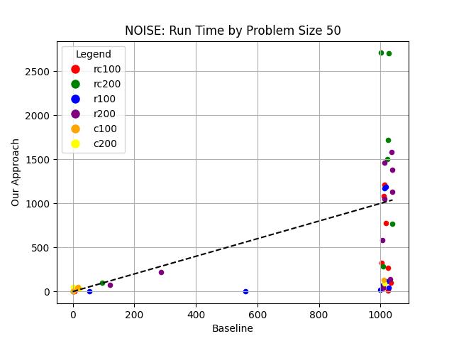
We provide comparisons across Solomon data sets/problem sizes in Figures 2(a)-2(b) (MILP time) and Figures 2(c)-2(d) (MILP+ all LPs time) Figures 2(e)-2(f) (integrality gap as a percentage). We define the integrality gap to be the difference between the MILP upper bound and the MILP Lower bound which are both produced over the course of running the MILP solver. For Figures 2(e)-2(f) we normalize the data as follows. We take integrality gap and divided it by the MILP upper bound then multiply by 100 to get the value to plot for both baseline and our approach. For problems with larger integrality gaps we believe that using valid inequalities to tighten the bound.In Figures 3(a)-3(b) we plot the LP integrality gap. We define this as the difference between the MILP upper bound and the LP at the root node of the branch & bound tree. We normalize the data as follows. We take LP integrality gap and divided it by the MILP upper bound then multiply by 100 to get the value to plot for both baseline and our approach. Since a large number of points for the baseline hit the 1000 second time horizon we had issues with visualization. Hence for such instances we add random noise to the baseline value for ILP run time and Total run time in Figs 3(c)-3(f).
We observe that LA-Discretization performs best relative to the baseline on problem instances which are hardest for baseline MILP to solve efficiently.


8 Conclusion
We have introduced a new approach for the Vehicle Routing Problem with Time Windows (VRPTW) called Local Area Discretization (LA-Discretization). This approach is designed to gain the advantages of the expanded (column generation) formulation for VRPTW (Desrochers et al., 1992) and the advantages of the compact two-index formulation without the associated disadvantages. Specifically we gain the advantages of the dramatically tighter LP relaxation of the expanded formulation while being able to solve optimization with an off-the-shelf MILP solver. This advantage should not be underestimated. Unlike related CG approaches no elaborate dual stabilization is required, nor are elaborate pricing algorithms for elementary resource constrained shortest path problems (Irnich and Desaulniers, 2005). However, we find that this method does not always lead to rapid identification of the optimal solution. In those cases we are close to optimal while the baseline is still far away.
Our solution is inspired by (Boland et al., 2017)’s work on time window discretization and pre-computation of component routes localized in space in (Mandal et al., 2022, 2023). Exploiting this approach applies time/capacity window discretization in the LP relaxation, and enforces that the solution to the compact LP is consistent with elementarity locally (hence eliminating sub-tours). LA-Discretization increases and decreases the discretization of time/capacity and the degree of enforcement of elementarity in such a manner as to produce an LP that is compact and tighter than a baseline compact formulation. However the vertices of the associated MILP can express every optimal solution to the original VRPTW. Hence solving this MILP exactly ensures an optimal solution to the original VRPTW. Utilizing LA-arcs for cycle removal in compact formulations stands out as a significant advancement, offering users the flexibility to scale up their formulations alongside the evolving computational prowess of MILP solvers.
In future work we intend to explore the use of valid inequalities such as subset-row inequalities (Jepsen et al., 2008; Wang et al., 2017) and rounded capacity inequalities (Archetti et al., 2011) for efficient tightening of the LP bound in a manner so as to exploit LA-arcs. We also intend to explore the use of alternative compact LP relaxations with our approach such as that of (Gavish and Graves, 1981). Furthermore we intend to explore the use of multiple LA-neighborhoods for customers in the same LP. We also intend to create a graph where nodes correspond to customers and NG neighbors (Baldacci et al., 2011) visited which keeps track of the route in an NG-neighbor like manner so as to further restrict cycles.
References
- Appelgren [1969] L. H. Appelgren. A column generation algorithm for a ship scheduling problem. Transportation Science, 3(1):53–68, 1969.
- Appelgren [1971] L. H. Appelgren. Integer programming methods for a vessel scheduling problem. Transportation Science, 5(1):64–78, 1971.
- Archetti et al. [2011] C. Archetti, N. Bianchessi, and M. G. Speranza. A column generation approach for the split delivery vehicle routing problem. Networks, 58(4):241–254, 2011.
- Baldacci et al. [2011] R. Baldacci, A. Mingozzi, and R. Roberti. New route relaxation and pricing strategies for the vehicle routing problem. Operations Research, 59(5):1269–1283, 2011.
- Baldacci et al. [2012] R. Baldacci, A. Mingozzi, and R. Roberti. Recent exact algorithms for solving the vehicle routing problem under capacity and time window constraints. European Journal of Operational Research, 218(1):1–6, 2012.
- Barnhart et al. [1996] C. Barnhart, E. L. Johnson, G. L. Nemhauser, M. W. P. Savelsbergh, and P. H. Vance. Branch-and-price: Column generation for solving huge integer programs. Operations Research, 46:316–329, 1996.
- Beasley and Christofides [1989] J. E. Beasley and N. Christofides. An algorithm for the resource constrained shortest path problem. Networks, 19(4):379–394, 1989.
- Boland et al. [2006] N. Boland, J. Dethridge, and I. Dumitrescu. Accelerated label setting algorithms for the elementary resource constrained shortest path problem. Operations Research Letters, 34(1):58–68, 2006.
- Boland et al. [2017] N. Boland, M. Hewitt, L. Marshall, and M. Savelsbergh. The continuous-time service network design problem. Operations Research, 65(5):1303–1321, 2017.
- Boland et al. [2019] N. Boland, M. Hewitt, L. Marshall, and M. Savelsbergh. The price of discretizing time: a study in service network design. EURO Journal on Transportation and Logistics, 8(2):195–216, 2019.
- Cabrera et al. [2020] N. Cabrera, A. L. Medaglia, L. Lozano, and D. Duque. An exact bidirectional pulse algorithm for the constrained shortest path. Networks, 76(2):128–146, 2020.
- Christofides et al. [1981] N. Christofides, A. Mingozzi, and P. Toth. Exact algorithms for the vehicle routing problem, based on spanning tree and shortest path relaxations. Mathematical programming, 20(1):255–282, 1981.
- Dantzig and Wolfe [1960] G. B. Dantzig and P. Wolfe. Decomposition principle for linear programs. Operations research, 8(1):101–111, 1960.
- Desaulniers et al. [1997] G. Desaulniers, J. Desrosiers, Y. Dumas, S. Marc, B. Rioux, M. M. Solomon, and F. Soumis. Crew pairing at air france. European journal of operational research, 97(2):245–259, 1997.
- Desrochers et al. [1992] M. Desrochers, J. Desrosiers, and M. Solomon. A new optimization algorithm for the vehicle routing problem with time windows. Operations Research, 40(2):342–354, 1992.
- Desrosiers and Lübbecke [2005] J. Desrosiers and M. E. Lübbecke. A primer in column generation. In G. Desaulniers, J. Desrosiers, and M. M. Solomon, editors, Column Generation, pages 1–32. Springer, New York, NY, 2005.
- Dollevoet et al. [2020] T. Dollevoet, P. Munari, and R. Spliet. A p-step formulation for the capacitated vehicle routing problem. Technical report, 2020.
- Du Merle et al. [1999] O. Du Merle, D. Villeneuve, J. Desrosiers, and P. Hansen. Stabilized column generation. Discrete Mathematics, 194(1-3):229–237, 1999.
- Gauvin et al. [2014] C. Gauvin, G. Desaulniers, and M. Gendreau. A branch-cut-and-price algorithm for the vehicle routing problem with stochastic demands. Computers & Operations Research, 50:141–153, 2014.
- Gavish and Graves [1981] B. Gavish and S. Graves. Scheduling and routing in transportation and distribution systems: formulations and new relaxations. Working Paper, 1981.
- Geoffrion [1974] A. M. Geoffrion. Lagrangean relaxation for integer programming. In Approaches to integer programming, pages 82–114. Springer, 1974.
- Ghoniem and Sherali [2009] A. Ghoniem and H. D. Sherali. Complementary column generation and bounding approaches for set partitioning formulations. Optimization Letters, 3:123–136, 2009.
- Gilmore and Gomory [1961] P. Gilmore and R. Gomory. A linear programming approach to the cutting-stock problem. Operations Research, 9(6):849–859, 1961.
- Haghani et al. [2022] N. Haghani, C. Contardo, and J. Yarkony. Smooth and flexible dual optimal inequalities. INFORMS Journal on Optimization, 4(1):29–44, 2022.
- Irnich and Desaulniers [2005] S. Irnich and G. Desaulniers. Shortest path problems with resource constraints. In G. Desaulniers, J. Desrosiers, and M. M. Solomon, editors, Column generation, pages 33–65. Springer, 2005.
- Jepsen et al. [2008] M. Jepsen, B. Petersen, S. Spoorendonk, and D. Pisinger. Subset-row inequalities applied to the vehicle-routing problem with time windows. Operations Research, 56(2):497–511, 2008.
- Li and Han [2019] J. Li and X. Han. Revised pulse algorithm for elementary shortest path problem with resource constraints. In 2019 seventh international symposium on computing and networking (CANDAR), pages 37–44. IEEE, 2019.
- Lokhande et al. [2020] V. S. Lokhande, S. Wang, M. Singh, and J. Yarkony. Accelerating column generation via flexible dual optimal inequalities with application to entity resolution. In Proceedings of the AAAI Conference on Artificial Intelligence, volume 34, pages 1593–1602, 2020.
- Lozano and Medaglia [2013] L. Lozano and A. L. Medaglia. On an exact method for the constrained shortest path problem. Computers & operations research, 40(1):378–384, 2013.
- Lozano et al. [2016] L. Lozano, D. Duque, and A. L. Medaglia. An exact algorithm for the elementary shortest path problem with resource constraints. Transportation Science, 50(1):348–357, 2016.
- Mandal et al. [2022] U. Mandal, A. Regan, and J. Yarkony. Local area routes and valid inequalities for efficient vehicle routing. arXiv preprint arXiv:2209.12963, 2022.
- Mandal et al. [2023] U. Mandal, A. Regan, L. M. Rousseau, and J. Yarkony. Graph master and local area routes for efficient column generation for the capacitated vehicle routing problem with time windows. arXiv preprint arXiv:2304.11723, 2023.
- Marsten et al. [1975] R. E. Marsten, W. Hogan, and J. W. Blankenship. The boxstep method for large-scale optimization. Operations Research, 23(3):389–405, 1975.
- Pecin et al. [2017] D. Pecin, A. Pessoa, M. Poggi, and E. Uchoa. Improved branch-cut-and-price for capacitated vehicle routing. Mathematical Programming Computation, 9(1):61–100, 2017.
- Righini and Salani [2004] G. Righini and M. Salani. Dynamic programming algorithms for the elementary shortest path problem with resource constraints. Electronic Notes in Discrete Mathematics, 17:247–249, 2004.
- Righini and Salani [2006] G. Righini and M. Salani. Symmetry helps: Bounded bi-directional dynamic programming for the elementary shortest path problem with resource constraints. Discrete Optimization, 3(3):255–273, 2006.
- Righini and Salani [2008] G. Righini and M. Salani. New dynamic programming algorithms for the resource constrained elementary shortest path problem. Networks: An International Journal, 51(3):155–170, 2008.
- Righini and Salani [2009] G. Righini and M. Salani. Decremental state space relaxation strategies and initialization heuristics for solving the orienteering problem with time windows with dynamic programming. Computers & Operations Research, 36(4):1191–1203, 2009.
- Rousseau et al. [2007] L.-M. Rousseau, M. Gendreau, and D. Feillet. Interior point stabilization for column generation. Operations Research Letters, 35(5):660–668, 2007.
- Solomon [1987] M. M. Solomon. Algorithms for the vehicle routing and scheduling problems with time window constraints. Operations research, 35(2):254–265, 1987.
- Tilk et al. [2017] C. Tilk, A.-K. Rothenbächer, T. Gschwind, and S. Irnich. Asymmetry matters: Dynamic half-way points in bidirectional labeling for solving shortest path problems with resource constraints faster. European Journal of Operational Research, 261(2):530–539, 2017.
- Wang et al. [2017] S. Wang, S. Wolf, C. Fowlkes, and J. Yarkony. Tracking objects with higher order interactions via delayed column generation. In Proc. 20th International Conference on Artificial Intelligence and Statistics, pages 1132–1140, Fort Lauderdale, Florida, 2017.
- Wang and Regan [2002] X. Wang and A. C. Regan. Local truckload pickup and delivery with hard time window constraints. Transportation Research Part B: Methodological, 36(2):97–112, 2002.
- Yarkony et al. [2020] J. Yarkony, Y. Adulyasak, M. Singh, and G. Desaulniers. Data association via set packing for computer vision applications. Informs Journal on Optimization, 2(3):167–191, 2020.
Appendix A Appendix/Extensions Overview
In this appendix we consider relevant proofs, derivations and extensions to the main document. We organize this appendix as follows. In Appendix B we provide a proof certifying the correctness of our approach to generating L-Arcs. In Appendix C we provide proof that bucket feasibility ensures a sufficient parameterization. In Appendix D we prove that Algorithm 1 converges to a sufficient parameterization. Appendix E provides additional experimental results directly related to this paper.
Appendix B Proof of Equivalent Representation of Departure Time
In this section we prove that (13) accurately characterizes for all . We prove this using induction. Observe that for the base case where that the claim holds by definition. If (13) does not hold for all cases then there must exist some s.t (13) does not hold but (13) holds for for all time. We describe this formally below using to denote the first two customers in .
Claim to be Proven False:
| (18) |
For now we assume (18) is true. We rew-write (14) below for reference
| (19) |
Proof: We now use (14) to replace in (18).
| (20) | |||
We now consider the terms corresponding to and those not corresponding to separately in (20). For the (18) to be true then it must be the case that . A necessary condition for (18) to be true is that one or both of the following must must be satisfied.
| (21a) | |||
| (21b) | |||
Let us consider (21a) first. We apply the following transformations including plugging in the definition of .
| (22a) | |||
| (22b) | |||
| (22c) | |||
Consider that then both the LHS and RHS of (22c) equal . Thus if a violation occurs in (22c) then . Thus we gain the following expression for a potential violation:
| (23) |
The only way for (23) to be satisfied is if . However both and are greater than or equal to creating a contradiction.
Appendix C Bucket Feasibility
Consider the following solution for where are equal to
For each in or we use when and when . For each we use to denote the edges in a lowest cost path in starting at and ending at where edges have cost defined by defined by . Similarly for each we use to denote the edges in a lowest cost path in starting at and ending at where edges are of cost defined by . Notice that for that contains exactly one edge for which and and no other edges between non-identical customers.
| (25a) | |||
| (25b) | |||
We now construct a feasible solution to optimization over given the LP over
Now initialize . Now iterate over and increase by for each in . Now iterate over and increase by for each in .
Observe that are feasible for ; and since only is in the objective that we have not changed the objective. Thus only violations in (6j),(6k),(6l),(6m) are possible. Observe that via (25a) that (6k) is obeyed and via and (25b) that (6m) is obeyed. Since the intermediate edges in the paths can be ignored then flow constraints (6j),(6l) are obeyed.
Appendix D Proof of Convergence to a Sufficient Parametization
In this section we establish that Alg 1 generates a sufficient parameterization when ITER_MAX=.
Observe that all expansion/contraction operations never decrease the primal objective. Thus Alg 1 monotonically increases the dual objective. Thus we need establish that Alg 1 can not converge to a value other than the maximum.
Observe that after iterations of not increasing the objective by MIN_INC that we have for all .
Given that for all observe Alg 1 can continue for a maximum of iterations before either the bound is increased or the buckets for time /capacity are at minimal granularity; thus producing a sufficient parameterization.
Appendix E All Results
We provide all timing results in this section for our data sets. We provide results on the Solomon instance data sets [Solomon, 1987].Each row describes the performance of the problem instance for a given approach. The baseline performance on a given instance is the row immediately below the row for LA-Discretization. We use the following columns to describe our results.
-
1.
File ID: We provide the problem instance ID.
-
2.
Approach: We indicate whether we used LA-Discretization or the Baseline MILP solver.
-
3.
LP Obj: This describes the root LP objective of the MILP being solved.
-
4.
MILP LB: This is the MILP dual bound at the termination of optimization.
-
5.
MILP Obj: This is the MILP objective at the termination of optimization,
-
6.
MILP time: This is the amount of time required to solve the MILP. Note that we cut off optimization at 1000 seconds. All times are rounded down to the nearest second.
-
7.
LP time: This is the time spent solving LPs over the course of LA-Discretization. This is the time required to solve the root LP for the baseline. All times are rounded down to the nearest second.
-
8.
10X: This is indicated as YES if LA-Discretization vastly outperforms the baseline for the given instance. We define vastly outperform as meeting the following two criteria (1) solving the optimization problem exactly and (2) doing so either ten times faster than the baseline or if the baseline does not finish during the allotted optimization time.
| file num | Approach | lp obj | mip dual bound | ILP obj | ilp time | total lp time | 10X+ |
|---|---|---|---|---|---|---|---|
| rc101 | OUR APPROACH | 402.8 | 461.1 | 461.1 | 0.1 | 0.3 | |
| rc101 | BASELINE MILP | 336.3 | 461.1 | 461.1 | 0.1 | 0.0 | |
| rc102 | OUR APPROACH | 350.9 | 351.8 | 351.8 | 0.1 | 0.7 | |
| rc102 | BASELINE MILP | 302.5 | 351.8 | 351.8 | 0.4 | 0.0 | |
| rc103 | OUR APPROACH | 319.2 | 332.8 | 332.8 | 0.4 | 3.1 | |
| rc103 | BASELINE MILP | 280.9 | 332.8 | 332.8 | 9.5 | 0.0 | |
| rc104 | OUR APPROACH | 302.0 | 306.6 | 306.6 | 0.3 | 2.1 | |
| rc104 | BASELINE MILP | 278.9 | 306.6 | 306.6 | 1.5 | 0.0 | |
| rc105 | OUR APPROACH | 408.5 | 411.3 | 411.3 | 0.1 | 0.6 | |
| rc105 | BASELINE MILP | 308.0 | 411.3 | 411.3 | 4.4 | 0.0 | |
| rc106 | OUR APPROACH | 334.7 | 345.5 | 345.5 | 0.5 | 4.7 | |
| rc106 | BASELINE MILP | 299.0 | 345.5 | 345.5 | 0.7 | 0.0 | |
| rc107 | OUR APPROACH | 297.8 | 298.3 | 298.3 | 0.1 | 2.1 | |
| rc107 | BASELINE MILP | 272.9 | 298.3 | 298.3 | 0.6 | 0.0 | |
| rc108 | OUR APPROACH | 293.7 | 294.5 | 294.5 | 0.7 | 16.9 | |
| rc108 | BASELINE MILP | 272.4 | 294.5 | 294.5 | 0.9 | 0.0 |
| file num | Approach | lp obj | mip dual bound | ILP obj | ilp time | total lp time | 10X+ |
|---|---|---|---|---|---|---|---|
| rc201 | OUR APPROACH | 358.8 | 360.2 | 360.2 | 0.0 | 0.2 | |
| rc201 | BASELINE MILP | 274.0 | 360.2 | 360.2 | 0.1 | 0.0 | |
| rc202 | OUR APPROACH | 307.3 | 338.0 | 338.0 | 1.5 | 10.1 | |
| rc202 | BASELINE MILP | 181.7 | 338.0 | 338.0 | 29.0 | 0.0 | |
| rc203 | OUR APPROACH | 259.6 | 326.9 | 326.9 | 329.4 | 34.6 | YES |
| rc203 | BASELINE MILP | 162.6 | 245.7 | 326.9 | 1000.0 | 0.0 | |
| rc204 | OUR APPROACH | 238.0 | 269.0 | 299.7 | 1000.1 | 11.8 | |
| rc204 | BASELINE MILP | 157.8 | 195.3 | 299.7 | 1000.0 | 0.0 | |
| rc205 | OUR APPROACH | 314.1 | 338.0 | 338.0 | 0.1 | 1.1 | |
| rc205 | BASELINE MILP | 193.7 | 338.0 | 338.0 | 0.4 | 0.0 | |
| rc206 | OUR APPROACH | 301.3 | 324.0 | 324.0 | 0.6 | 2.8 | |
| rc206 | BASELINE MILP | 183.2 | 324.0 | 324.0 | 1.7 | 0.0 | |
| rc207 | OUR APPROACH | 254.5 | 298.3 | 298.3 | 34.8 | 14.4 | YES |
| rc207 | BASELINE MILP | 153.7 | 274.2 | 298.3 | 1000.0 | 0.0 | |
| rc208 | OUR APPROACH | 168.1 | 186.0 | 269.1 | 1000.0 | 17.4 | |
| rc208 | BASELINE MILP | 148.3 | 190.0 | 269.1 | 1000.0 | 0.0 |
| file num | Approach | lp obj | mip dual bound | ILP obj | ilp time | total lp time | 10X+ |
|---|---|---|---|---|---|---|---|
| r101 | OUR APPROACH | 617.1 | 617.1 | 617.1 | 0.0 | 0.0 | |
| r101 | BASELINE MILP | 617.1 | 617.1 | 617.1 | 0.0 | 0.0 | |
| r102 | OUR APPROACH | 546.3 | 547.1 | 547.1 | 0.0 | 0.1 | |
| r102 | BASELINE MILP | 384.7 | 547.1 | 547.1 | 0.4 | 0.0 | |
| r103 | OUR APPROACH | 454.2 | 454.6 | 454.6 | 0.1 | 0.9 | |
| r103 | BASELINE MILP | 328.9 | 454.6 | 454.6 | 3.9 | 0.0 | |
| r104 | OUR APPROACH | 415.0 | 416.9 | 416.9 | 0.1 | 1.4 | YES |
| r104 | BASELINE MILP | 319.5 | 416.9 | 416.9 | 36.2 | 0.0 | |
| r105 | OUR APPROACH | 530.5 | 530.5 | 530.5 | 0.0 | 0.0 | |
| r105 | BASELINE MILP | 456.5 | 530.5 | 530.5 | 0.1 | 0.0 | |
| r106 | OUR APPROACH | 457.3 | 465.4 | 465.4 | 0.1 | 0.3 | |
| r106 | BASELINE MILP | 346.3 | 465.4 | 465.4 | 0.6 | 0.0 | |
| r107 | OUR APPROACH | 417.4 | 424.3 | 424.3 | 0.1 | 1.8 | |
| r107 | BASELINE MILP | 319.7 | 424.3 | 424.3 | 6.8 | 0.0 | |
| r108 | OUR APPROACH | 391.7 | 397.3 | 397.3 | 0.2 | 5.5 | |
| r108 | BASELINE MILP | 311.0 | 397.3 | 397.3 | 20.4 | 0.0 | |
| r109 | OUR APPROACH | 440.3 | 441.3 | 441.3 | 0.1 | 0.4 | |
| r109 | BASELINE MILP | 347.3 | 441.3 | 441.3 | 0.2 | 0.0 | |
| r110 | OUR APPROACH | 421.5 | 444.1 | 444.1 | 1.0 | 2.7 | YES |
| r110 | BASELINE MILP | 312.8 | 444.1 | 444.1 | 65.8 | 0.0 | |
| r111 | OUR APPROACH | 418.4 | 428.8 | 428.8 | 0.2 | 1.8 | |
| r111 | BASELINE MILP | 320.6 | 428.8 | 428.8 | 5.3 | 0.0 | |
| r112 | OUR APPROACH | 371.3 | 393.0 | 393.0 | 2.2 | 9.7 | YES |
| r112 | BASELINE MILP | 309.9 | 393.0 | 393.0 | 353.0 | 0.0 |
| file num | Approach | lp obj | mip dual bound | ILP obj | ilp time | total lp time | 10X+ |
|---|---|---|---|---|---|---|---|
| r201 | OUR APPROACH | 458.6 | 463.3 | 463.3 | 0.0 | 0.4 | |
| r201 | BASELINE MILP | 417.0 | 463.3 | 463.3 | 0.0 | 0.0 | |
| r202 | OUR APPROACH | 399.6 | 410.5 | 410.5 | 0.2 | 2.0 | |
| r202 | BASELINE MILP | 314.7 | 410.5 | 410.5 | 1.5 | 0.0 | |
| r203 | OUR APPROACH | 362.5 | 391.4 | 391.4 | 0.9 | 8.8 | |
| r203 | BASELINE MILP | 302.3 | 391.4 | 391.4 | 43.0 | 0.0 | |
| r204 | OUR APPROACH | 322.2 | 355.0 | 355.0 | 2.5 | 15.7 | |
| r204 | BASELINE MILP | 292.6 | 355.0 | 355.0 | 29.6 | 0.0 | |
| r205 | OUR APPROACH | 386.4 | 393.0 | 393.0 | 0.1 | 2.4 | |
| r205 | BASELINE MILP | 337.9 | 393.0 | 393.0 | 0.6 | 0.0 | |
| r206 | OUR APPROACH | 349.2 | 374.4 | 374.4 | 1.7 | 11.3 | |
| r206 | BASELINE MILP | 292.9 | 374.4 | 374.4 | 5.1 | 0.0 | |
| r207 | OUR APPROACH | 338.4 | 361.6 | 361.6 | 2.9 | 23.3 | |
| r207 | BASELINE MILP | 292.4 | 361.6 | 361.6 | 11.2 | 0.0 | |
| r208 | OUR APPROACH | 312.3 | 328.2 | 328.2 | 2.0 | 8.1 | |
| r208 | BASELINE MILP | 292.3 | 328.2 | 328.2 | 2.9 | 0.0 | |
| r209 | OUR APPROACH | 354.6 | 370.7 | 370.7 | 0.9 | 5.3 | |
| r209 | BASELINE MILP | 303.3 | 370.7 | 370.7 | 0.8 | 0.0 | |
| r210 | OUR APPROACH | 378.3 | 404.6 | 404.6 | 1.9 | 9.5 | |
| r210 | BASELINE MILP | 302.7 | 404.6 | 404.6 | 1.8 | 0.0 | |
| r211 | OUR APPROACH | 313.6 | 350.9 | 350.9 | 19.2 | 19.1 | |
| r211 | BASELINE MILP | 292.4 | 350.9 | 350.9 | 44.7 | 0.0 |
| file num | Approach | lp obj | mip dual bound | ILP obj | ilp time | total lp time | 10X+ |
|---|---|---|---|---|---|---|---|
| c101 | OUR APPROACH | 191.3 | 191.3 | 191.3 | 0.0 | 0.1 | |
| c101 | BASELINE MILP | 191.3 | 191.3 | 191.3 | 0.0 | 0.0 | |
| c102 | OUR APPROACH | 190.3 | 190.3 | 190.3 | 0.0 | 0.4 | |
| c102 | BASELINE MILP | 172.7 | 190.3 | 190.3 | 0.2 | 0.0 | |
| c103 | OUR APPROACH | 190.3 | 190.3 | 190.3 | 0.1 | 2.0 | |
| c103 | BASELINE MILP | 163.8 | 190.3 | 190.3 | 0.6 | 0.0 | |
| c104 | OUR APPROACH | 186.9 | 186.9 | 186.9 | 0.1 | 2.8 | |
| c104 | BASELINE MILP | 160.5 | 186.9 | 186.9 | 2.4 | 0.0 | |
| c105 | OUR APPROACH | 191.3 | 191.3 | 191.3 | 0.0 | 0.1 | |
| c105 | BASELINE MILP | 191.2 | 191.3 | 191.3 | 0.0 | 0.0 | |
| c106 | OUR APPROACH | 191.3 | 191.3 | 191.3 | 0.0 | 0.1 | |
| c106 | BASELINE MILP | 191.3 | 191.3 | 191.3 | 0.0 | 0.0 | |
| c107 | OUR APPROACH | 191.3 | 191.3 | 191.3 | 0.0 | 0.1 | |
| c107 | BASELINE MILP | 191.2 | 191.3 | 191.3 | 0.0 | 0.0 | |
| c108 | OUR APPROACH | 191.3 | 191.3 | 191.3 | 0.0 | 1.1 | |
| c108 | BASELINE MILP | 131.5 | 191.3 | 191.3 | 0.2 | 0.0 | |
| c109 | OUR APPROACH | 190.6 | 191.3 | 191.3 | 0.2 | 6.4 | |
| c109 | BASELINE MILP | 131.1 | 191.3 | 191.3 | 0.8 | 0.0 |
| file num | Approach | lp obj | mip dual bound | ILP obj | ilp time | total lp time | 10X+ |
|---|---|---|---|---|---|---|---|
| c201 | OUR APPROACH | 214.7 | 214.7 | 214.7 | 0.0 | 0.1 | |
| c201 | BASELINE MILP | 214.7 | 214.7 | 214.7 | 0.0 | 0.0 | |
| c202 | OUR APPROACH | 214.7 | 214.7 | 214.7 | 0.0 | 2.0 | |
| c202 | BASELINE MILP | 175.0 | 214.7 | 214.7 | 0.6 | 0.0 | |
| c203 | OUR APPROACH | 214.7 | 214.7 | 214.7 | 0.0 | 3.3 | |
| c203 | BASELINE MILP | 169.5 | 214.7 | 214.7 | 1.5 | 0.0 | |
| c204 | OUR APPROACH | 209.6 | 213.1 | 213.1 | 1.0 | 8.6 | |
| c204 | BASELINE MILP | 165.4 | 213.1 | 213.1 | 24.9 | 0.0 | |
| c205 | OUR APPROACH | 214.7 | 214.7 | 214.7 | 0.0 | 0.3 | |
| c205 | BASELINE MILP | 176.4 | 214.7 | 214.7 | 0.0 | 0.0 | |
| c206 | OUR APPROACH | 214.7 | 214.7 | 214.7 | 0.0 | 0.5 | |
| c206 | BASELINE MILP | 173.1 | 214.7 | 214.7 | 0.2 | 0.0 | |
| c207 | OUR APPROACH | 211.3 | 214.5 | 214.5 | 0.2 | 5.8 | |
| c207 | BASELINE MILP | 166.7 | 214.5 | 214.5 | 1.0 | 0.0 | |
| c208 | OUR APPROACH | 211.7 | 214.5 | 214.5 | 0.1 | 1.1 | |
| c208 | BASELINE MILP | 166.4 | 214.5 | 214.5 | 0.3 | 0.0 |
| file num | Approach | lp obj | mip dual bound | ILP obj | ilp time | total lp time | 10X+ |
|---|---|---|---|---|---|---|---|
| rc101 | OUR APPROACH | 841.4 | 944.0 | 944.0 | 2.7 | 3.8 | |
| rc101 | BASELINE MILP | 610.6 | 944.0 | 944.0 | 5.3 | 0.0 | |
| rc102 | OUR APPROACH | 710.2 | 822.5 | 822.5 | 303.9 | 24.7 | YES |
| rc102 | BASELINE MILP | 515.9 | 751.5 | 822.5 | 1000.0 | 0.0 | |
| rc103 | OUR APPROACH | 623.0 | 672.2 | 710.9 | 1000.0 | 73.6 | |
| rc103 | BASELINE MILP | 480.0 | 575.3 | 711.5 | 1000.0 | 0.0 | |
| rc104 | OUR APPROACH | 529.8 | 545.8 | 545.8 | 56.9 | 208.9 | YES |
| rc104 | BASELINE MILP | 467.6 | 523.2 | 545.8 | 1000.0 | 0.0 | |
| rc105 | OUR APPROACH | 747.9 | 855.3 | 855.3 | 6.8 | 8.5 | YES |
| rc105 | BASELINE MILP | 533.6 | 791.8 | 855.3 | 1000.1 | 0.0 | |
| rc106 | OUR APPROACH | 648.5 | 723.2 | 723.2 | 27.1 | 69.7 | YES |
| rc106 | BASELINE MILP | 500.9 | 618.3 | 723.2 | 999.9 | 0.0 | |
| rc107 | OUR APPROACH | 573.3 | 642.7 | 642.7 | 616.1 | 157.3 | YES |
| rc107 | BASELINE MILP | 470.9 | 559.0 | 642.7 | 1000.0 | 0.0 | |
| rc108 | OUR APPROACH | 528.4 | 536.2 | 598.1 | 1000.0 | 208.0 | |
| rc108 | BASELINE MILP | 463.2 | 502.7 | 599.4 | 1000.0 | 0.0 |
| file num | Approach | lp obj | mip dual bound | ILP obj | ilp time | total lp time | 10X+ |
|---|---|---|---|---|---|---|---|
| rc201 | OUR APPROACH | 677.9 | 684.8 | 684.8 | 0.2 | 2.0 | |
| rc201 | BASELINE MILP | 385.5 | 684.8 | 684.8 | 0.8 | 0.0 | |
| rc202 | OUR APPROACH | 539.8 | 613.6 | 613.6 | 591.1 | 180.3 | YES |
| rc202 | BASELINE MILP | 296.3 | 522.1 | 613.6 | 1000.0 | 0.0 | |
| rc203 | OUR APPROACH | 437.6 | 474.0 | 555.3 | 1000.0 | 463.5 | |
| rc203 | BASELINE MILP | 257.3 | 365.2 | 557.3 | 1000.0 | 0.0 | |
| rc204 | OUR APPROACH | 307.0 | 315.1 | 449.8 | 1000.0 | 1683.8 | |
| rc204 | BASELINE MILP | 237.0 | 273.9 | 444.2 | 1000.0 | 0.0 | |
| rc205 | OUR APPROACH | 569.4 | 630.2 | 630.2 | 34.1 | 69.3 | |
| rc205 | BASELINE MILP | 366.8 | 630.2 | 630.2 | 95.5 | 0.0 | |
| rc206 | OUR APPROACH | 521.2 | 610.0 | 610.0 | 153.6 | 133.2 | YES |
| rc206 | BASELINE MILP | 292.2 | 586.0 | 610.0 | 1000.0 | 0.0 | |
| rc207 | OUR APPROACH | 462.5 | 483.5 | 561.5 | 1000.0 | 692.5 | |
| rc207 | BASELINE MILP | 255.3 | 341.7 | 560.2 | 1000.0 | 0.0 | |
| rc208 | OUR APPROACH | 283.8 | 292.5 | 493.8 | 1000.2 | 1682.9 | |
| rc208 | BASELINE MILP | 229.2 | 265.5 | 517.7 | 1000.0 | 0.0 |
| file num | Approach | lp obj | mip dual bound | ILP obj | ilp time | total lp time | 10X+ |
|---|---|---|---|---|---|---|---|
| r101 | OUR APPROACH | 1044.0 | 1044.0 | 1044.0 | 0.0 | 0.1 | |
| r101 | BASELINE MILP | 1029.8 | 1044.0 | 1044.0 | 0.0 | 0.0 | |
| r102 | OUR APPROACH | 909.0 | 909.0 | 909.0 | 0.1 | 1.2 | YES |
| r102 | BASELINE MILP | 649.7 | 909.0 | 909.0 | 54.9 | 0.0 | |
| r103 | OUR APPROACH | 762.1 | 772.9 | 772.9 | 3.1 | 12.7 | YES |
| r103 | BASELINE MILP | 533.1 | 721.7 | 772.9 | 1000.0 | 0.0 | |
| r104 | OUR APPROACH | 612.1 | 625.4 | 625.4 | 22.7 | 95.3 | YES |
| r104 | BASELINE MILP | 464.6 | 541.6 | 636.0 | 1000.0 | 0.0 | |
| r105 | OUR APPROACH | 898.5 | 911.8 | 911.8 | 0.3 | 0.8 | |
| r105 | BASELINE MILP | 793.0 | 911.8 | 911.8 | 1.2 | 0.0 | |
| r106 | OUR APPROACH | 792.7 | 793.0 | 793.0 | 0.3 | 4.1 | YES |
| r106 | BASELINE MILP | 547.0 | 793.0 | 793.0 | 561.0 | 0.0 | |
| r107 | OUR APPROACH | 700.5 | 711.1 | 711.1 | 4.4 | 37.1 | YES |
| r107 | BASELINE MILP | 483.2 | 631.7 | 724.4 | 1000.0 | 0.0 | |
| r108 | OUR APPROACH | 584.9 | 608.1 | 617.7 | 1000.0 | 160.2 | |
| r108 | BASELINE MILP | 457.5 | 530.6 | 624.7 | 1000.0 | 0.0 | |
| r109 | OUR APPROACH | 752.1 | 786.8 | 786.8 | 9.5 | 37.9 | YES |
| r109 | BASELINE MILP | 547.2 | 767.5 | 786.8 | 1000.0 | 0.0 | |
| r110 | OUR APPROACH | 681.1 | 697.0 | 697.0 | 9.9 | 68.5 | YES |
| r110 | BASELINE MILP | 481.0 | 606.3 | 713.0 | 1000.0 | 0.0 | |
| r111 | OUR APPROACH | 673.0 | 707.2 | 707.2 | 35.5 | 31.5 | YES |
| r111 | BASELINE MILP | 475.4 | 603.8 | 714.2 | 1000.0 | 0.0 | |
| r112 | OUR APPROACH | 593.3 | 613.9 | 630.2 | 1000.0 | 146.8 | |
| r112 | BASELINE MILP | 451.8 | 513.2 | 647.9 | 1000.0 | 0.0 |
| file num | Approach | lp obj | mip dual bound | ILP obj | ilp time | total lp time | 10X+ |
|---|---|---|---|---|---|---|---|
| r201 | OUR APPROACH | 789.5 | 791.9 | 791.9 | 0.1 | 3.5 | |
| r201 | BASELINE MILP | 700.9 | 791.9 | 791.9 | 0.3 | 0.0 | |
| r202 | OUR APPROACH | 680.5 | 698.5 | 698.5 | 6.6 | 39.4 | YES |
| r202 | BASELINE MILP | 504.4 | 682.4 | 698.5 | 1000.0 | 0.0 | |
| r203 | OUR APPROACH | 570.2 | 605.3 | 605.3 | 36.1 | 104.7 | YES |
| r203 | BASELINE MILP | 447.9 | 540.0 | 605.9 | 1000.0 | 0.0 | |
| r204 | OUR APPROACH | 464.6 | 487.8 | 508.1 | 1000.0 | 378.8 | |
| r204 | BASELINE MILP | 420.4 | 477.4 | 508.9 | 1000.0 | 0.0 | |
| r205 | OUR APPROACH | 662.2 | 690.1 | 690.1 | 6.7 | 65.9 | |
| r205 | BASELINE MILP | 540.9 | 690.1 | 690.1 | 120.7 | 0.0 | |
| r206 | OUR APPROACH | 584.4 | 632.4 | 632.4 | 445.2 | 141.4 | YES |
| r206 | BASELINE MILP | 455.2 | 581.8 | 639.0 | 1000.0 | 0.0 | |
| r207 | OUR APPROACH | 519.9 | 556.5 | 576.1 | 1000.0 | 438.9 | |
| r207 | BASELINE MILP | 420.6 | 521.6 | 575.5 | 1000.0 | 0.0 | |
| r208 | OUR APPROACH | 455.6 | 468.1 | 487.7 | 1000.0 | 118.7 | |
| r208 | BASELINE MILP | 412.1 | 469.9 | 494.2 | 1000.0 | 0.0 | |
| r209 | OUR APPROACH | 568.6 | 600.6 | 600.6 | 64.7 | 153.6 | |
| r209 | BASELINE MILP | 481.2 | 600.6 | 600.6 | 287.4 | 0.0 | |
| r210 | OUR APPROACH | 592.8 | 645.6 | 645.6 | 841.9 | 211.2 | YES |
| r210 | BASELINE MILP | 456.2 | 591.2 | 647.8 | 1000.0 | 0.0 | |
| r211 | OUR APPROACH | 489.8 | 504.6 | 540.9 | 1000.0 | 563.4 | |
| r211 | BASELINE MILP | 412.1 | 479.3 | 541.3 | 1000.0 | 0.0 |
| file num | Approach | lp obj | mip dual bound | ILP obj | ilp time | total lp time | 10X+ |
|---|---|---|---|---|---|---|---|
| c101 | OUR APPROACH | 362.4 | 362.4 | 362.4 | 0.1 | 0.5 | |
| c101 | BASELINE MILP | 361.4 | 362.4 | 362.4 | 0.0 | 0.0 | |
| c102 | OUR APPROACH | 361.4 | 361.4 | 361.4 | 0.2 | 2.4 | |
| c102 | BASELINE MILP | 334.0 | 361.4 | 361.4 | 0.5 | 0.0 | |
| c103 | OUR APPROACH | 361.4 | 361.4 | 361.4 | 0.8 | 40.3 | |
| c103 | BASELINE MILP | 284.7 | 361.4 | 361.4 | 15.1 | 0.0 | |
| c104 | OUR APPROACH | 355.2 | 358.0 | 358.0 | 11.9 | 118.5 | YES |
| c104 | BASELINE MILP | 281.0 | 312.4 | 358.0 | 1000.0 | 0.0 | |
| c105 | OUR APPROACH | 362.4 | 362.4 | 362.4 | 0.1 | 1.2 | |
| c105 | BASELINE MILP | 360.0 | 362.4 | 362.4 | 0.1 | 0.0 | |
| c106 | OUR APPROACH | 362.4 | 362.4 | 362.4 | 0.1 | 0.9 | |
| c106 | BASELINE MILP | 360.1 | 362.4 | 362.4 | 0.1 | 0.0 | |
| c107 | OUR APPROACH | 362.4 | 362.4 | 362.4 | 0.1 | 1.7 | |
| c107 | BASELINE MILP | 360.0 | 362.4 | 362.4 | 0.1 | 0.0 | |
| c108 | OUR APPROACH | 362.4 | 362.4 | 362.4 | 0.2 | 6.2 | |
| c108 | BASELINE MILP | 261.1 | 362.4 | 362.4 | 0.9 | 0.0 | |
| c109 | OUR APPROACH | 361.7 | 362.4 | 362.4 | 1.8 | 51.0 | |
| c109 | BASELINE MILP | 257.1 | 362.4 | 362.4 | 16.1 | 0.0 |
| file num | Approach | lp obj | mip dual bound | ILP obj | ilp time | total lp time | 10X+ |
|---|---|---|---|---|---|---|---|
| c201 | OUR APPROACH | 360.2 | 360.2 | 360.2 | 0.0 | 0.9 | |
| c201 | BASELINE MILP | 360.2 | 360.2 | 360.2 | 0.0 | 0.0 | |
| c202 | OUR APPROACH | 360.2 | 360.2 | 360.2 | 0.1 | 11.9 | |
| c202 | BASELINE MILP | 318.2 | 360.2 | 360.2 | 2.0 | 0.0 | |
| c203 | OUR APPROACH | 359.8 | 359.8 | 359.8 | 0.2 | 35.5 | |
| c203 | BASELINE MILP | 299.1 | 359.8 | 359.8 | 22.5 | 0.0 | |
| c204 | OUR APPROACH | 349.9 | 350.1 | 350.1 | 0.8 | 89.8 | YES |
| c204 | BASELINE MILP | 288.6 | 345.8 | 350.1 | 1000.0 | 0.0 | |
| c205 | OUR APPROACH | 359.8 | 359.8 | 359.8 | 0.1 | 2.5 | |
| c205 | BASELINE MILP | 313.1 | 359.8 | 359.8 | 0.2 | 0.0 | |
| c206 | OUR APPROACH | 359.8 | 359.8 | 359.8 | 0.1 | 4.4 | |
| c206 | BASELINE MILP | 310.9 | 359.8 | 359.8 | 0.9 | 0.0 | |
| c207 | OUR APPROACH | 356.5 | 359.6 | 359.6 | 1.8 | 49.4 | |
| c207 | BASELINE MILP | 310.7 | 359.6 | 359.6 | 1.3 | 0.0 | |
| c208 | OUR APPROACH | 347.4 | 350.5 | 350.5 | 0.2 | 7.7 | |
| c208 | BASELINE MILP | 309.0 | 350.5 | 350.5 | 0.8 | 0.0 |
| file num | Approach | lp obj | mip dual bound | ILP obj | ilp time | total lp time | 10X+ |
|---|---|---|---|---|---|---|---|
| rc101 | OUR APPROACH | 1577.3 | 1619.8 | 1619.8 | 17.8 | 28.8 | |
| rc101 | BASELINE MILP | 1131.3 | 1619.8 | 1619.8 | 316.1 | 0.1 | |
| rc102 | OUR APPROACH | 1384.2 | 1431.9 | 1457.4 | 1000.1 | 126.4 | |
| rc102 | BASELINE MILP | 795.6 | 1098.7 | 1481.6 | 1000.0 | 0.0 | |
| rc103 | OUR APPROACH | 1176.8 | 1185.9 | 1288.1 | 1000.0 | 320.6 | |
| rc103 | BASELINE MILP | 694.5 | 857.3 | 1389.1 | 1000.1 | 0.1 | |
| rc104 | OUR APPROACH | 1050.6 | 1060.8 | 1227.4 | 1000.0 | 327.8 | |
| rc104 | BASELINE MILP | 670.4 | 782.6 | 1197.0 | 1000.1 | 0.1 | |
| rc105 | OUR APPROACH | 1461.4 | 1513.7 | 1513.7 | 94.9 | 52.3 | YES |
| rc105 | BASELINE MILP | 927.5 | 1268.4 | 1552.8 | 1000.0 | 0.0 | |
| rc106 | OUR APPROACH | 1269.2 | 1294.2 | 1373.5 | 1000.1 | 133.0 | |
| rc106 | BASELINE MILP | 782.3 | 1018.0 | 1411.6 | 1000.1 | 0.0 | |
| rc107 | OUR APPROACH | 1125.0 | 1139.8 | 1260.9 | 1000.1 | 333.8 | |
| rc107 | BASELINE MILP | 681.9 | 803.0 | 1358.8 | 1000.1 | 0.1 | |
| rc108 | OUR APPROACH | 1041.3 | 1047.3 | 1235.9 | 1000.1 | 319.9 | |
| rc108 | BASELINE MILP | 663.1 | 738.0 | 1217.6 | 999.4 | 0.1 |
| file num | Approach | lp obj | mip dual bound | ILP obj | ilp time | total lp time | 10X+ |
|---|---|---|---|---|---|---|---|
| rc201 | OUR APPROACH | 1214.0 | 1261.8 | 1261.8 | 6.8 | 90.1 | |
| rc201 | BASELINE MILP | 946.2 | 1261.8 | 1261.8 | 119.0 | 0.0 | |
| rc202 | OUR APPROACH | 963.6 | 1008.1 | 1100.7 | 1000.4 | 428.7 | |
| rc202 | BASELINE MILP | 659.9 | 863.3 | 1124.3 | 1000.0 | 0.0 | |
| rc203 | OUR APPROACH | 764.0 | 779.5 | 1088.5 | 1000.0 | 305.4 | |
| rc203 | BASELINE MILP | 575.8 | 702.1 | 976.7 | 1000.1 | 0.1 | |
| rc204 | OUR APPROACH | 647.3 | 655.4 | 943.0 | 1000.1 | 312.3 | |
| rc204 | BASELINE MILP | 544.5 | 628.9 | 812.4 | 1000.0 | 0.1 | |
| rc205 | OUR APPROACH | 1045.5 | 1083.8 | 1159.2 | 1000.0 | 317.5 | |
| rc205 | BASELINE MILP | 759.1 | 1029.0 | 1178.1 | 1000.0 | 0.0 | |
| rc206 | OUR APPROACH | 951.1 | 969.7 | 1058.1 | 1000.0 | 414.7 | |
| rc206 | BASELINE MILP | 710.3 | 905.4 | 1066.7 | 1000.0 | 0.0 | |
| rc207 | OUR APPROACH | 841.5 | 857.2 | 1060.3 | 1000.0 | 309.2 | |
| rc207 | BASELINE MILP | 602.0 | 738.3 | 988.1 | 1000.0 | 0.1 | |
| rc208 | OUR APPROACH | 646.0 | 652.6 | 995.3 | 1000.0 | 324.3 | |
| rc208 | BASELINE MILP | 536.8 | 609.2 | 854.5 | 1000.0 | 0.1 |
| file num | Approach | lp obj | mip dual bound | ILP obj | ilp time | total lp time | 10X+ |
|---|---|---|---|---|---|---|---|
| r101 | OUR APPROACH | 1631.2 | 1637.7 | 1637.7 | 0.3 | 1.1 | |
| r101 | BASELINE MILP | 1612.2 | 1637.7 | 1637.7 | 0.1 | 0.0 | |
| r102 | OUR APPROACH | 1467.7 | 1467.7 | 1467.7 | 1.0 | 10.3 | YES |
| r102 | BASELINE MILP | 1027.2 | 1320.4 | 1470.5 | 1000.0 | 0.0 | |
| r103 | OUR APPROACH | 1204.2 | 1208.7 | 1208.7 | 9.1 | 65.6 | YES |
| r103 | BASELINE MILP | 787.2 | 999.1 | 1244.2 | 1000.0 | 0.1 | |
| r104 | OUR APPROACH | 944.9 | 946.5 | 1060.0 | 1000.0 | 338.2 | |
| r104 | BASELINE MILP | 693.1 | 780.2 | 1012.8 | 1000.0 | 0.1 | |
| r105 | OUR APPROACH | 1341.6 | 1355.3 | 1355.3 | 5.6 | 24.0 | YES |
| r105 | BASELINE MILP | 1098.2 | 1355.3 | 1355.3 | 440.9 | 0.0 | |
| r106 | OUR APPROACH | 1215.4 | 1234.6 | 1234.6 | 70.2 | 95.6 | YES |
| r106 | BASELINE MILP | 833.3 | 1016.2 | 1266.9 | 1000.0 | 0.1 | |
| r107 | OUR APPROACH | 1040.6 | 1049.8 | 1070.6 | 1000.0 | 201.7 | |
| r107 | BASELINE MILP | 719.2 | 827.8 | 1126.8 | 1000.1 | 0.1 | |
| r108 | OUR APPROACH | 906.9 | 908.6 | 1151.9 | 999.9 | 411.1 | |
| r108 | BASELINE MILP | 679.8 | 736.3 | 997.1 | 1000.0 | 0.1 | |
| r109 | OUR APPROACH | 1109.3 | 1136.7 | 1146.9 | 1000.0 | 109.2 | |
| r109 | BASELINE MILP | 775.6 | 939.7 | 1194.9 | 1000.0 | 0.0 | |
| r110 | OUR APPROACH | 1028.8 | 1034.9 | 1078.8 | 1000.2 | 188.2 | |
| r110 | BASELINE MILP | 704.3 | 794.3 | 1115.9 | 1000.0 | 0.1 | |
| r111 | OUR APPROACH | 1012.7 | 1026.3 | 1050.6 | 1000.0 | 193.2 | |
| r111 | BASELINE MILP | 704.0 | 803.5 | 1126.2 | 1000.0 | 0.1 | |
| r112 | OUR APPROACH | 910.0 | 911.1 | 1070.6 | 1000.0 | 438.7 | |
| r112 | BASELINE MILP | 668.9 | 716.6 | 1069.9 | 1000.1 | 0.1 |
| file num | Approach | lp obj | mip dual bound | ILP obj | ilp time | total lp time | 10X+ |
|---|---|---|---|---|---|---|---|
| r201 | OUR APPROACH | 1114.0 | 1143.2 | 1143.2 | 5.0 | 119.5 | |
| r201 | BASELINE MILP | 979.2 | 1143.2 | 1143.2 | 21.2 | 0.0 | |
| r202 | OUR APPROACH | 974.2 | 1006.9 | 1029.6 | 1000.0 | 362.9 | |
| r202 | BASELINE MILP | 731.0 | 872.7 | 1049.5 | 1000.0 | 0.0 | |
| r203 | OUR APPROACH | 794.0 | 809.0 | 883.2 | 1000.0 | 636.0 | |
| r203 | BASELINE MILP | 633.0 | 716.7 | 906.3 | 1000.0 | 0.1 | |
| r204 | OUR APPROACH | 668.0 | 675.8 | 770.1 | 1000.0 | 804.5 | |
| r204 | BASELINE MILP | 591.1 | 647.9 | 789.8 | 1000.1 | 0.1 | |
| r205 | OUR APPROACH | 891.0 | 912.4 | 954.7 | 1000.0 | 473.6 | |
| r205 | BASELINE MILP | 738.1 | 879.8 | 967.4 | 1000.0 | 0.0 | |
| r206 | OUR APPROACH | 803.7 | 825.6 | 898.0 | 1000.0 | 798.7 | |
| r206 | BASELINE MILP | 651.9 | 758.2 | 914.6 | 1000.0 | 0.1 | |
| r207 | OUR APPROACH | 719.4 | 728.3 | 900.0 | 1000.0 | 1687.1 | |
| r207 | BASELINE MILP | 612.2 | 691.4 | 815.7 | 1000.1 | 0.1 | |
| r208 | OUR APPROACH | 643.2 | 645.4 | 823.4 | 1000.0 | 396.1 | |
| r208 | BASELINE MILP | 583.6 | 643.7 | 729.6 | 1000.0 | 0.1 | |
| r209 | OUR APPROACH | 790.8 | 804.2 | 905.7 | 1000.0 | 339.0 | |
| r209 | BASELINE MILP | 653.0 | 758.1 | 859.2 | 1000.0 | 0.1 | |
| r210 | OUR APPROACH | 808.6 | 826.3 | 934.0 | 1000.0 | 407.7 | |
| r210 | BASELINE MILP | 644.9 | 760.2 | 928.6 | 1000.0 | 0.1 | |
| r211 | OUR APPROACH | 667.5 | 672.0 | 881.2 | 1000.0 | 292.8 | |
| r211 | BASELINE MILP | 583.6 | 642.3 | 799.2 | 1000.1 | 0.1 |
| file num | Approach | lp obj | mip dual bound | ILP obj | ilp time | total lp time | 10X+ |
|---|---|---|---|---|---|---|---|
| c101 | OUR APPROACH | 827.3 | 827.3 | 827.3 | 0.2 | 2.9 | |
| c101 | BASELINE MILP | 819.7 | 827.3 | 827.3 | 0.1 | 0.1 | |
| c102 | OUR APPROACH | 827.1 | 827.3 | 827.3 | 1.8 | 47.7 | |
| c102 | BASELINE MILP | 754.3 | 827.3 | 827.3 | 24.1 | 0.0 | |
| c103 | OUR APPROACH | 826.1 | 826.3 | 826.3 | 19.0 | 136.8 | YES |
| c103 | BASELINE MILP | 588.9 | 785.0 | 826.3 | 1000.0 | 0.1 | |
| c104 | OUR APPROACH | 818.2 | 822.9 | 822.9 | 195.5 | 170.5 | YES |
| c104 | BASELINE MILP | 577.2 | 673.3 | 830.1 | 1000.0 | 0.1 | |
| c105 | OUR APPROACH | 827.3 | 827.3 | 827.3 | 0.3 | 3.2 | |
| c105 | BASELINE MILP | 818.2 | 827.3 | 827.3 | 0.1 | 0.0 | |
| c106 | OUR APPROACH | 827.3 | 827.3 | 827.3 | 0.4 | 10.9 | |
| c106 | BASELINE MILP | 699.7 | 827.3 | 827.3 | 0.7 | 0.0 | |
| c107 | OUR APPROACH | 827.3 | 827.3 | 827.3 | 0.5 | 5.9 | |
| c107 | BASELINE MILP | 818.1 | 827.3 | 827.3 | 0.4 | 0.0 | |
| c108 | OUR APPROACH | 827.3 | 827.3 | 827.3 | 5.0 | 71.2 | |
| c108 | BASELINE MILP | 569.5 | 827.3 | 827.3 | 8.4 | 0.0 | |
| c109 | OUR APPROACH | 825.1 | 827.3 | 827.3 | 54.8 | 145.2 | YES |
| c109 | BASELINE MILP | 566.0 | 792.1 | 853.4 | 1000.0 | 0.1 |
| file num | Approach | lp obj | mip dual bound | ILP obj | ilp time | total lp time | 10X+ |
|---|---|---|---|---|---|---|---|
| c201 | OUR APPROACH | 589.1 | 589.1 | 589.1 | 0.1 | 5.5 | |
| c201 | BASELINE MILP | 589.1 | 589.1 | 589.1 | 0.1 | 0.0 | |
| c202 | OUR APPROACH | 589.1 | 589.1 | 589.1 | 0.3 | 65.6 | |
| c202 | BASELINE MILP | 556.7 | 589.1 | 589.1 | 1.6 | 0.1 | |
| c203 | OUR APPROACH | 583.7 | 588.7 | 588.7 | 13.9 | 127.4 | |
| c203 | BASELINE MILP | 534.9 | 588.7 | 588.7 | 6.0 | 0.1 | |
| c204 | OUR APPROACH | 582.4 | 588.1 | 588.1 | 61.6 | 183.7 | |
| c204 | BASELINE MILP | 517.5 | 588.1 | 588.1 | 77.8 | 0.1 | |
| c205 | OUR APPROACH | 586.0 | 586.4 | 586.4 | 0.3 | 29.5 | |
| c205 | BASELINE MILP | 539.7 | 586.4 | 586.4 | 0.4 | 0.0 | |
| c206 | OUR APPROACH | 586.0 | 586.0 | 586.0 | 0.2 | 33.1 | |
| c206 | BASELINE MILP | 536.3 | 586.0 | 586.0 | 2.1 | 0.0 | |
| c207 | OUR APPROACH | 582.7 | 585.8 | 585.8 | 5.2 | 98.5 | |
| c207 | BASELINE MILP | 535.7 | 585.8 | 585.8 | 2.0 | 0.0 | |
| c208 | OUR APPROACH | 583.4 | 585.8 | 585.8 | 1.0 | 72.0 | |
| c208 | BASELINE MILP | 531.9 | 585.8 | 585.8 | 3.3 | 0.0 |