A new approach for extracting information from protein dynamics
Network inference from protein dynamics
Abstract
Increased ability to predict protein structures is moving research focus towards understanding protein dynamics. A promising approach is to represent protein dynamics through networks and take advantage of well-developed methods from network science. Most studies build protein dynamics networks from correlation measures, an approach that only works under very specific conditions, instead of the more robust inverse approach. Thus, we apply the inverse approach to the dynamics of protein dihedral angles, a system of internal coordinates, to avoid structural alignment. Using the well-characterized adhesion protein, FimH, we show that our method identifies networks that are physically interpretable, robust, and relevant to the allosteric pathway sites. We further use our approach to detect dynamical differences, despite structural similarity, for Siglec-8 in the immune system, and the SARS-CoV-2 spike protein. Our study demonstrates that using the inverse approach to extract a network from protein dynamics yields important biophysical insights.
Keywords
Molecular Dynamics Simulation; Protein; SARS-CoV-2; Sialic Acid Binding Immunoglobulin-like Lectins; Fimbrial Adhesins
Statements
Data available on request from the authors. We have no conflict of interest to declare.
Acknowledgments
The authors thank Martin Gerlach and Kerim Dansuk for helpful conversations. J.L. thanks the Paul and Daisy Soros Fellowship, the Northwestern Quest High Performance Computing Cluster, and the National Institute of Health T32GM008152. This project was also supported by the Office of Naval Research N00014163175 and N000141512701 (S.K.), the National Science Foundation 2034584 (S.K.) and 1764421-01 (L.A.N.L.), and the Simons Foundation 597491-01 (L.A.N.L.).
Introduction
Advances in experimental structure determination 1, 2, computational structure prediction 3, and molecular dynamics simulations 4 have set the stage for high-throughput characterization of protein dynamics using molecular dynamics (MD) simulations. Combined with increased computational power, these advances have led to rapidly increasing numbers of longer MD simulations for larger macromolecular systems 5. As a result, large datasets of MD trajectories are available from individual research labs 5 and repositories such as MoDEL 6, Dynameomics 7, Dryad, NoMaD, and MolSSI 8.
This wealth of MD trajectory data creates opportunities for expanding our understanding of protein dynamics and function. While snapshots from MD trajectories contain information about low energy states and can be used to identify conformational changes, some physical phenomena – such as dynamic allostery in proteins – may be better characterized by dynamics over the course of the trajectory 9. MD simulations can capture differences among protein variants, the impact of mutations, and modulation by small molecule binding at spatiotemporal resolutions that are difficult, or even impossible, to obtain experimentally 4.
Taking advantage of this growing wealth of MD trajectory data will require the development of robust methods for automated analysis. A common strategy for analyzing dynamics data involves creating a network by directly calculating contact times and interaction energies 10, 11, 12, 13. An alternative strategy used in network science aims to identify the underlying interactions of multi-component systems by inferring a network structure from dynamics 14. Compared to interaction energy networks, building networks from dynamics is typically less computationally expensive and avoids less rigorous modeling of water or entropic contributions to the free energy 15. Identifying a network structure makes it possible to apply network analysis tools in order to uncover emergent properties such as densely-connected communities 16, hotspots with many edges 17, and paths connecting active sites and allosteric regulatory sites in distant protein regions 11, 18.
In the study of proteins, the typical approach for constructing networks from protein MD simulations has made use of correlation measures that quantify how different protein regions ”move together.” These include a variety of methods that use linear 19 and non-linear 20, 21, 22, 23, 24, 17 correlation measures. Yet a rigorous mathematical analysis demonstrates that inferring the network structure by solving the inverse problem for a system that could produce the observed correlations is a more accurate approach than using the correlations directly 14. The most straightforward form of solving the inverse problem is simply calculating the inverse of the covariance matrix 14. Here we apply the inverse covariance approach to MD trajectory data.
A remaining challenge is how to define the nodes in such a network representation. An approach that has been used in proteins is to assign a node to each C atom in elastic network models 25, 26 . This choice has some appeal because the model describes “beads”, located in Cartesian coordinates, connected by linear springs 25, 26. However, using Cartesian coordinates requires a structural alignment step that can introduce ”artifacts” during hinged motion for multi-domain proteins, and even for small, single-domain proteins 27. Previously, we have demonstrated that an internal coordinate system using dihedral angles makes it possible to accurately localize motion that affects elements distal to the hinge in fimH 28.
Here, we show that network inference using inverse covariance analysis is robust across replicates and that it uncovers strong interactions among backbone dihedrals that form a contact-map pattern. While the contact-map pattern is also seen in elastic network models for single domains with high conformational stability, we continue to see this pattern even for multi-domain proteins with hinged motion when using inverse covariance analysis.
We demonstrate the value of the proposed approach by studying three physiologically significant proteins: the bacterial adhesion protein, FimHL, the human immune adhesion protein Siglec-8 29, and two domains of the SARS-CoV-2 spike protein involved in adhesion to the human ACE2 receptor 30. In addition to comparing the different structures of wild type and mutant FimHL, we are also able to detect localized structural changes due to breaking a disulfide bond in silico. For Siglec-8, we are able to detect differences between “apo” and “holo” states, despite their structural similarity 29. For the SARS-CoV-2 spike protein, we examined the receptor binding domain (RBD) and its connecting subdomain 1 (SD1). While the hinge region connecting RBD-SD1 is open in the up state and closed in the down state, the individual domains remain structurally similar in the up and down states 30. For Siglec-8 and spike RBD-SD1, which do not have large structural changes within protein domains, comparing inferred networks allowed us to identify dynamical changes and contributions to stability.
Materials and Methods
Protein structures
We retrieved crystal structure for FimHL wild type and mutant, Siglec-8 apo and holo, and SARS-CoV-2 spike protein from the Protein Data Bank, as detailed in Table 1. For FimHL, we used crystal structures of the lectin domain without ligand for both the wild type and the mutant. To compare dynamics with and without the disulfide bond as a local perturbation, we used Visual Molecular Dynamics (VMD) to define the bond or two cystines for FimHL. For Siglec-8, we simulated the ligand 6’S sLex without the 3-amino-propyl linker, which is not thought to interact with the binding pocket 29.
For the SARS-CoV-2 spike protein, we started from the refined structure on the CHARMM-GUI archive 31, 30. To focus on one hinge system that is thought to be different between the down and up states, we isolated the receptor binding domain (RBD) and subdomain 1 (SD1) protein subunits without the glycans. For the up state, we used chain A where the RBD is accessible for binding the ACE2 receptor on human cells 30, and for the down state, we used chain B. We used the structure
We prepared all systems using VMD version 1.9.3 32. We solvated each protein with at least 16 Å of TIP3P water molecules on each side to prevent interactions with itself through the periodic boundary conditions. We added sodium and chloride ions to neutralize the system and achieve the desired salt concentration in Table 1.
MD simulations
We performed all-atomistic MD simulations using NAMD 33, with the CHARMM force field34. Our NAMD simulation parameters and system details are listed in Table 2.
| Protein | FimH | Siglec-8 | Spike RBD-SD1 | |||||
|---|---|---|---|---|---|---|---|---|
| Type | Crystal | NMR | Cryo-EM | |||||
| [NaCl] (mM) | 50 | 150 | 150 | |||||
| State | Wild type | Mutant | Full-length | Apo | Holo | Up | Down | Off |
| PDBID | 4AUU | 5MCA | 4XOD | 2N7A | 2N7B | 6VSB | 6VSB | 6VXX |
| Protein residues | 158 | 158 | 279 | 145 | 276 | |||
| Protein atoms | 2,360 | 2,350 | 4,270 | 2,290 | 4,286 | |||
| System atoms | 32,292 | 31,917 | 60,376 | 42,684 | 50,879 | 80,383 | 89,236 | 78,740 |
| System size | 94 | 87 | 123 | 97 | 111 | 125 | 116 | 115 |
| 61 | 67 | 72 | 70 | 72 | 94 | 95 | 94 | |
| 59 | 59 | 72 | 67 | 67 | 81 | 81 | 77 | |
| Parameter | Value | |||
|---|---|---|---|---|
| Setup | VMD 1.9.3 (RRID:SCR_004905) | |||
| Simulation engine | NAMD 2.13 (RRID:SCR_014894) | |||
| Ensemble | NPT | |||
| Temperature | 300 K | |||
| Pressure | 1 atm | |||
| Non-bonded interactions | Lennard-Jones potential ( cutoff) | |||
| Electrostatic interactions | Particle-Mesh Ewald sum method | |||
| Forcefield | CHARMM c36 July 2018 update | |||
| Timestep | 1 fs | |||
| Coordinate saved every | 1 ps | |||
| Energy minimization |
|
After observing differences in correlated protein motions between replicates, we performed three replicates of over 200 ns each for wild type FimHL. Due to the tradeoff between the number replicates and simulation length, we performed six replicates of 20 ns of FimHL to make comparisons of wild type and mutant FimH, as well as wild type FimH with and without the Cys3-Cys44 disulfide bond.
Since twenty lowest-energy structures are reported for Siglec-8, we performed a single replicate of 50 ns for each structure to compare apo and holo Siglec-8. For the spike RBD-SD1 domains, we performed six replicates of 60 ns.
Backbone and sidechain dihedral angle dynamics
We used dihedral angles to capture protein dynamics because dihedral angles identify localized regions responsible for the collective displacement of regions distal from the angular rotation, such as in hinged motion 35. Dihedral angles are also an internal coordinate system that avoids the structure alignment step when using Cartesian coordinates, which can introduce artifacts 27. We use both backbone () and sidechain () dihedral angles. We extracted protein features with MDTraj 1.9.5.
Inverse of the covariance matrix
In the literature, the covariance matrix is one approach used to identify protein regions with motions that are related to the motions of many other regions; in particular it is used to identify correlated motions between distant regions in allostery 22, 36. However, constructing networks from the covariance matrix, even with a threshold to remove weak correlations, is susceptible to induced correlations when two nodes (e.g. A and C) are not directly connected but share a connection with a third node (B) 14. Borrowing from the field of network reconstruction, we use the inverse of the covariance matrix to identify the connections and weights, or edges, between nodes 14. This approach is consistent with finding the inverse of a covariance matrix based on C positions, which fits the Hessian matrix describing an elastic spring network with anisotropy 25, 26. We have found that the anisotropic elastic network model (ANM) has large errors when used to describe the motion of FimH, which is consistent with errors for hinge-motion described in literature 37. As a result, we use dihedral angles. This approach is similar to the torsional network model (TNM) which uses equal spring constants to describe dihedral angles across the protein 38. In contrast, the inverse of the covariance matrix uses the variances and the covariances of angles to calculate spring constants for a network of torsional springs. The nodes in our network are dihedral angles, the edges are like linearly coupled torsional springs, and the inverse of the covariance matrix is the Hessian matrix for a TNM.
To construct our network, we calculate the Moore-Penrose pseudo-inverse of the covariance matrix using both the backbone and sidechain dihedral angles. We use this approach to understand the relative contributions of backbone and sidechain dynamics to collective motion. Since the sign describes whether the angles turn in the same direction, we take the absolute value to get the interaction strength. We do not apply distance filters. While we use the 97th percentile as a value threshold for selecting strong interactions or visualizing the network on the protein, we do not use any thresholds for network comparisons. More generally, we recommend caution for applying thresholds to these networks for analysis.
Comparing networks of inferred interactions
To identify interactions that are stronger in one protein state than another, we compare each edge. We select for large differences between groups, relative to the variability within each group. To do this, we filter for differences larger than twice the standard deviation for each group. To compare an edge between states and , each with an ensemble of and networks, this is and . We apply this rule without determining statistical significance with corrections for multiple comparisons, in order to see the full effects of comparing all interactions on the matrix. In Supplementary Figure 11, we also show an example of comparisons without filtering for large differences, in order to illustrate the persistence of the contact-map pattern. We perform the network comparisons in two ways: 1) for every edge on the network (see Supplementary Figure 11), 2) accounting for the multi-layer structure of the network by collapsing the backbone-backbone interactions into residue-residue interactions (Figure 4). We analyzed data in python, using SciPy (RRID:SCR_008058) and custom packages.
Results
We present results below for these three proteins (Figure 1A). We first focus on the well-characterized allosteric protein FimHL. Separation of the FimHL domain from its connecting domain (bottom in all figures) is thought to induce an allosteric conformational change on the opposite end of the protein (top in figures) 39, 40. This changes the binding pocket from a state with low affinity for the ligand to one with high affinity (Figure 1B) 39. While wild type FimHL is trapped in the high-affinity state, a single-amino acid mutation (Arg60Pro) stabilizes FimHL in the low-affinity state 41, 42. The mutant FimHL is of interest because it undergoes an allostery-like conformational change upon binding mannoside ligands and has been proposed as a minimal model of allostery 42.
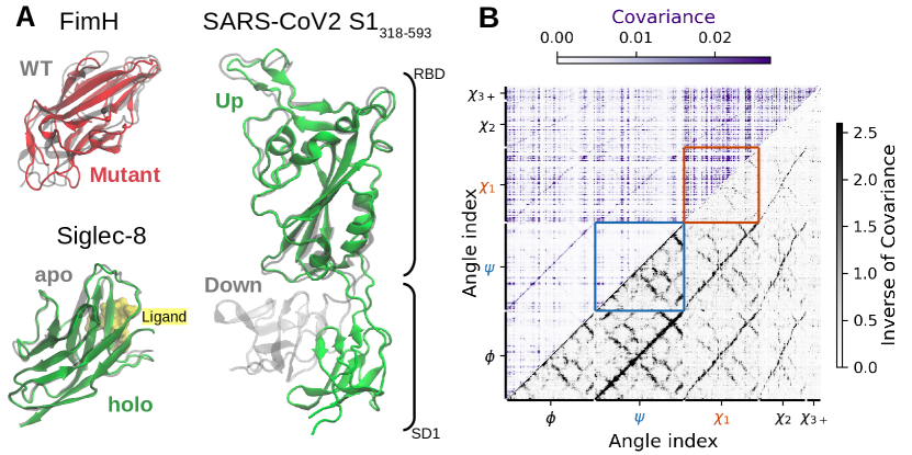
Like FimHL, Siglec-8 binds a carbohydrate ligand and has an immunoglobulin-like fold with two -sheets (Figure 1C). Functionally however, Siglec-8 binds to specific sugars found uniquely in human airway tissues to prevent autoimmunity 29, 43. For specific binding, Siglec-8 has a surprisingly rigid binding pocket loop, leading to similar structures for the apo and holo states 29. The SARS-CoV-2 spike protein RBD binds the human ACE2 receptor with a ”hook” region44. The hook becomes accessible in the up state when the hinge between the RBD and its connector opens (Figure 1A). While the hook and interdomain hinge regions are flexible, the bulk of the RBD is thought to be structurally similar in the up and down states. Both Siglec-8 and the spike RBD-SD1 present challenges for detecting differences in inferred interactions because the protein state changes without major structural changes within domains.
Define and validate network inference from inverse covariance analysis
Our approach for constructing a network representation of the dynamics of a given protein is comprised of three steps. In the first step, we obtain temporal dynamics for the nodes, which are the backbone (, ) and sidechain () dihedral angles for each residue 24, 35. In the second step, we calculate the circular covariance for dihedral angles 35, which can be thought of as the linearization of the interactions captured by mutual information. In the third step, we invert the covariance matrix using the Moore-Penrose pseudo-inverse to calculate the best fit for a linear coupling system that can give rise to the observed covariance matrix 14.
Similar to mutual information calculations conducted on other proteins 24, 17, we find that backbone-backbone interactions computed from the covariance are weak compared to sidechain-sidechain interactions (compare red and blue boxes in Figure 1B and the mutual information in Figure S4). In these networks, some dihedral angles have a banding pattern, suggesting long-range interactions with many other dihedral angles (Figure 1B and Figure S1). In contrast, the inverse covariance matrix has localized and specific interactions. In addition, the stronger backbone-backbone interactions have a repeating pattern that resembles the contact map of the protein, and this pattern appears to repeat more weakly in backbone-sidechain interactions.
The banding pattern in the covariance matrix is also widespread in mutual information matrices, where they have been interpreted as long-range interactions important in protein allostery 24, 17. The large number of long-distance edges produce ”hairball” networks, which led to the use of pruning algorithms 45, 46 or distance filters 22, 36, 47 in prior studies, in order to make network analysis tractable. Thus, we wondered whether the long-range interactions are capturing a physical feature of the dynamics. To answer this question, we investigate the reproducibility of the covariance, correlation, and inverse covariance matrices extracted from different replicates of MD simulations.
In Figure 2A, we contrast the matrix for one replicate in the upper-diagonal with the second replicate in the lower-diagonal and quantify the similarity in Figure 2B. For replicate MD simulations, we used the same initial protein structure with randomized solvation and initial velocities. Both covariance matrices have banding patterns suggesting hotspots that interact with many residues across the protein. However, each replicate has its own banding pattern, with interaction strengths that are over ten times greater than those found in the other replicate, indicating high variability in the networks that one would construct from replicate simulations.

Since the banding pattern is associated with dihedral angles with high variance, we also consider the correlation matrix, which normalizes the covariance matrix by the variance of each dihedral angle. It is visually apparent that the banding in the covariance matrix is not simply due to high variance because there are still bands in the correlation matrix. While normalizing to the correlation matrix uncovers some interactions in a contact map pattern, they are weak compared to the banding pattern (see Figure S5 for a lower maximum value on the color map scale).
In contrast to the irreproducible results obtained with the covariance matrix, for the inverse of the covariance matrix, we find a pattern that is visually similar to the 12Å contact map (Figure 2C). The diagonally symmetric contact map pattern in blue indicates similarly strong interactions for two replicates (Figure 2A). After quantifying the robustness across three replicates using the Jaccard similarity index, we find that the inverse covariance has higher similarity (59-72% shared edges) than the covariance (8-10%) or the correlation (13-16%) for backbone interactions (Figure 2B). The similarity values for inverse covariance are lower, but still higher than for the other two methods. These data clearly demonstrate that networks inferred from inverse covariance analysis are more robust than networks constructed from correlational measures.
Inverse covariance analysis yields structural networks
Prompted by the strong visual resemblance between the inverse covariance network and the 12Å contact map and the complete absence of this pattern in the covariance network, we wondered if the inverse covariance matrix could be used to identify specific physical interactions. To answer this question, we overlaid the strongest edges ( 97th percentile) on the 12Å contact map, highlighting the backbone-backbone edges as blue dots and the sidechain-sidechain edges as red crosses (Figure 3A and Figure S10).
To correct for the high variability across replicates we previously found for the covariance networks, we averaged networks across the three replicates. Despite the averaging, the covariance network shows strong interactions across distant protein regions and are dominated by interactions.

To understand how these contrasting patterns affect interpretation, we next visualize strong interactions as edges drawn on the protein structure (Figure 3B). Since drawing all edges would make the covariance network indecipherable, we only show the edges originating from Lys4. In contrast, the inverse covariance network uncovers edges that mostly connect physically close residues. Specifically, we find a edge between Cys3-Cys44 for the sole disulfide bond in FimHL, and that this edge is missing from the covariance network (red vs green arrow in Figure 3A).
Examining the contact map pattern of the inverse covariance network in more detail, we compare edge weight with the distance between C atoms (Figure S9). We find that for backbone-backbone interactions, the strongest interactions are between residues connected by a peptide bond, followed by hydrogen bonds within sheets, and then non-bonding interactions.
After examining backbone-backbone interactions, we next looked at the progressively weaker interactions involving sidechains distal from the backbone (Figure 1B and Figure S10). We find the contact map pattern is still apparent for or interactions, but becomes very weak for or interactions, and becomes indistinguishable from noise for interactions between proximal and distal sidechain dihedrals. The inverse covariance analysis thus suggests that backbone dihedral motion is most strongly coupled to nearby backbone dihedrals and has more dissipated effects on sidechain dihedrals. This relationship is consistent with how backbone motions can sterically trap or free sidechains, whereas sidechain motions are more limited in their impact on backbone motion 48.
The different strengths of interactions for backbone-backbone and backbone-sidechain edges suggests that qualitatively different types of interactions have different properties. For two residues i and j, the backbone-backbone edge are larger than the backbone-sidechain edge , which is consistent with the physical differences between these two edge types. Moreover, most backbone-backbone edges within the same residue, , are stronger than backbone edges connecting to other residues, [i, j] and [i, j] (Figure S9).
Detecting both large and small structural changes in FimHL
Conformational differences between wild type and mutant
As a way to further validate our approach, we next test if we are able to identify the well-characterized differences between wild type FimHL and the Arg60Pro mutant. To compare inferred networks for the wild type and mutant proteins, we identified edges where the average difference was larger than two times the standard deviation across each group of replicates. We performed this analysis once with the entire set of edges (Figure S11), and again with only the backbone interactions collapsed into a residue interaction network. For our comparisons and the matrix visualization of the differences, we do not apply a distance filter or a threshold for the edge-strength. However, for the visualization on the protein, we only show differences with magnitude larger than the 97th percentile.
The visualization of the differences enables us to identify several interactions stronger in either the mutant or the wild type proteins (red or blue patches, respectively, in Figure 4A). This is consistent with the difference in initial structure (RMSD=3.15Å), dihedral dynamics 28, and the residues that are rearranged in the allosteric conformational change 41, 49.

For concreteness, we focus on two regions at the edge of the protein structure that are easier to visualize: the binding pocket zipper at the top of FimHL, and the insertion loop at the bottom. In the pocket zipper, we found much stronger interactions for the mutant protein (median:2.8-fold, IQR:2.0–5.2-fold), which correspond to smaller dihedral fluctuations 28. On the other hand, in the insertion loop, we identified changes in interaction that were stronger in the wild type than the mutant protein (3.2-fold, 2.2–3.7-fold). Structurally, this is consistent with how the insertion loop is stabilized in the wild type structure and exposed to solvent in the mutant protein 50, 42. Dynamically, stronger interactions within the insertion loop is consistent with smaller dihedral fluctuations in the wild type protein 28.
We further identify differences at the -bulge, -switch, and swing loop regions of the allosteric pathway, consistent with structural differences between wild type and mutant proteins. The mutant protein has stronger interactions within the loop formed by the -bulge (2.0-fold, 1.2–2.3-fold) and also with a nearby loop. In the wild type protein, the loop is smoothed out into a -strand. The wild type protein has stronger interactions (1.8-fold, 1.5–2.6-fold) in the -helix, compared to the -helix in the mutant protein, which is probably due to different hydrogen bonding patterns. In the swing loop, we again find stronger interactions in the wild type protein (2.0-fold, 1.6–2.7-fold).
For these allosteric pathway landmarks, it is visually apparent that we detect large differences in inferred interactions when structures are closer in one state and stretched apart in the other state. Beyond these regions, there are several other regions with similarly large changes in interaction between the wild type and mutant proteins, shown in blue and red patches (Figure 4A).
Quantifying the impact of disulfide bond reduction
We next used wild type FimHL to explore the impact of reducing the single disulfide bond between Cys3-Cys44 in silico on fast, nanosecond-timescale dynamics. Using the inverse covariance analysis, we correctly identified the 6-fold stronger - interactions in the presence of the disulfide bond, which was the largest difference detected (Figure 4D). This matches our expectations because the covalent bond between the most distal atoms forming the rotamer angle directly couples dynamics. Together, these analyses show that the inverse covariance analysis method is sensitive to both local differences and conformational differences.
Network inference detects key mechanisms involved in Siglec-8 binding
Like FimHL, the human immune cell adhesion protein, Siglec-8, is also a lectin with an immunoglobulin-like fold with a single disulfide bond. For Siglec-8, we compare the apo (no ligand) and holo (bound to the native 6’S-sLex ligand) states. Due to the rigid binding pocket loop that only differs by a few sidechain rearrangements, apo and holo Siglec-8 have extremely similar structures29. Intriguingly, the rigidity of the CC’ binding pocket loop in apo Siglec-8 occurs in the absence of stabilizing secondary structure motifs 29 and plays a major role in recognizing specific ligands in the airway to avoid autoimmunity 43.
One hypothesized mechanism for stabilizing the CC’ loop in apo Siglec-8 is that the Arg70 sidechain forms hydrogen bonds with the loop backbone at Pro57 and Asp60 (Figure 5A)29. We identified Arg70-Pro57 or Arg70-Asp60 hydrogen bonds with occupancy between 10-33% in seven out of 20 simulations from the ensemble of NMR structures, and higher occupancy (80 and 83%) in only two simulations. This suggests the hydrogen bond is rarely present. Nonetheless, the unstructured CC’ loop has surprisingly small fluctuations across the ensemble of MD simulations (Figure 5B-E).

Using our inferred interaction networks, we identified strong interactions within the CC’ loop, as well as interactions from outside the loop to its hinges at Ala53 and Pro62 (Figure S12). Consistent with the hydrogen bonding analysis, we only identified strong interactions with Arg70 in a few MD simulations, which disappeared after averaging the networks across the ensemble. Counter-intuitively, in the two structures where Arg70 does form stable hydrogen bonds with Pro57 and Asp60, the CC’ loop has paradoxically larger fluctuations, especially at Tyr58 and Gln59 at the loop tip (Figure S12). Taken together, we suspect that steric hindrance plays a role in stabilizing the CC’ loop internally and externally at the hinge edges.
Of note, this example demonstrates an instance where the inferred network approach provides more clarity than contact or interaction energy networks, because the inverse of the covariance matrix identifies the degrees of freedom that most strongly affect the fluctuations at the CC’ loop.
After examining why the CC’ loop is similar in apo and holo Siglec-8, we next compared inferred networks for the apo and holo states. The holo state has stronger - interactions corresponding to the Cys31-Cys91 disulfide bond (Figure 5C and Figure S13). The disulfide bond is conserved in the siglec family and is located on the sheet of the -sandwich opposite the binding pocket 29. Nearby, we also observe other changes in interaction strength involving Asp90. Although distant from the binding site, the Asp90-Cys91-Ser92 motif in Siglec-8 is a variant of the Asn-Cys-Ser or -Thr motif that is conserved in the rest of the siglec family 51. Differences in interaction strength between apo and holo states identify changes in the dynamics of this evolutionarily conserved region during ligand-binding.
In contrast, reducing the Cys31-Cys91 disulfide bond in the holo state in silico has a different pattern (Figure S13). Both ligand-binding and the presence of the disulfide bond correspond to stronger a - interaction at Cys31-Cys91. Both conditions also stabilize Cys31, indicated by decreased backbone dihedral fluctuations and increased duration within an extended secondary structure as assigned by the DSSP algorithm, and shorter Cys31-Cys91 C distance. Taken together, we find that the network rearrangement that occurs with ligand-binding increases Siglec-8 conformational stability near an evolutionarily conserved disulfide bond, even though the region is not near the binding site.
Comparison of the spike protein RBD-SD1 fragments in the up, down, and off states shows network rearrangements without large structural differences
Next, we investigated whether there are differences in the networks inferred from the ‘up’, ‘down’, and ‘off’ states of the RBD-SD1 domains of the SARS-CoV-2 spike protein (Figure 1A). The RBD connects to SD1 (Fig 5E) via two hinge-like loops that are more flexible in the up state than in the down or off states 52. While the up state has a different orientation around the hinge than the down and off states, they all have similar SD1 structures (C-RMSD 0.64Å) and somewhat similar RBD structures (C-RMSD 1.55Å).
Opening the hinge angle in the down-to-up transition is thought to make the binding site on the RBD available to attach to human ACE2 30, 44. To focus on the RBD-SD1 hinge, we isolated these domains from the rest of the spike protein and ignored glycosylated sugars. While these simplifications limit the strength of our conclusions into the function of the spike protein, the RBD-SD1 structures nonetheless provide a useful system for comparing dynamics in a system that initially resembles rigid-body motion around a hinge.
Since the trimeric spike protein with one exposed RBD has two hidden RBDs, we isolated one RBD-SD1 fragment in the ‘up’ state, and two fragments in the ‘down’ state. We obtained another RBD-SD1 domain in the ‘off’ state from a structure with all RBDs hidden and 3-fold rotational symmetry. We first compared the RBD-SD1 fragments in the down and off conformations. Despite the structural similarity, we nevertheless detect differences in the inferred networks (Fig 5E) based on dynamics. We find the networks for the two down conformations are more similar to each other than to the networks for the off conformation (Figure S15).
We next compared RBD-SD1 fragments in the down and off conformations to the fragment in the up conformation (Figure S15). Surprisingly, we find that the differences in inferred networks among the down and up conformations are more localized, while the networks for the off conformation are distinct from the others. The localized differences are in the hook of the RBD that is exposed in the up conformation, and at an -helix near the RBD-SD1 hinge. Intriguingly, we also identified differences in the structural orientation and the inferred network interaction at the Cys336-Cys361 disulfide bond. In this region, one down conformation is more similar to the up conformation, while the other down conformation resembles the off conformation (Fig 5E).
As a proof-of-concept, we investigated whether it is possible to infer an interaction network for the trimeric SARS-CoV-2 spike protein, even though it is much larger than the RBD-SD1 domains. However, the amount of data required for network inference using the inverse covariance method scales faster than the number of residues. As a result, our approach required more data than was available from the two sets of publicly-accessible simulations for which the up and down states are labeled 53, 54. Instead, we chose the longer simulations that explore the transition among the down, up, and open states published by the Bowman lab 55. Using 100,000 snapshots, we were able to infer an interaction network for the 3,363 residues of the spike protein (Figure S14). The number of snapshots is an order of magnitude larger than those currently available for labeled states. Thus, it may be feasible to compare states for the entire S1/S2 complex of the spike protein if there is sufficient data, or by choosing a less data-intensive method for solving the inverse problem.
Discussion
We identify some of the shortcomings of correlation-based approaches for network inference from protein dynamics using the covariance, correlation, and mutual information matrices. These networks have low reproducibility among replicates and exhibit long-range connections that are difficult to tie to physical explanations. To address these shortcomings, we use the inverse of the covariance matrix. This is a well-established technique from network inference14 for solving the inverse problem for a system that can produce the observed correlated dynamics. Our approach builds networks where each node is a dihedral angle, including both the backbone (, ) and the sidechains (), and edges are inferred from the coupling interactions between angles. We chose the internal coordinate system of dihedral angles35 to easily include sidechain dynamics, localize hinges that drive distal dynamics28, and to avoid the alignment step in Cartesian coordinates that introduces ‘artifacts’ in hinged motion 37.
Using the inverse covariance approach, we detected differences in conformation, subtle differences between protein states without large conformational changes, and localized perturbations in the structure of biomedically important proteins. The inverse covariance networks capture a hierarchy of interactions that resemble that qualitatively different types of interactions, suggesting a multi-layer network structure. The strongest edges connect dihedral angles with covalently-bonded atoms, with weaker interactions for greater distances. Moreover, the contact map-like pattern found in backbone-backbone interactions are repeated more weakly in backbone-sidechain and sidechain-sidechain interactions. This hierarchy of inferred interactions is consistent with the view that smaller backbone rearrangements related to larger sidechain motions 48.
Our results suggest that solving the inverse problem uncovers the underlying interactions that ultimately drive protein dynamics, but are not well-captured by cataloguing the observed correlated motions or comparing static structures. Notably, inverting the covariance matrix is the simplest of a variety of tools available for network inference from dynamics used in network science 14, 56. While the simplicity of inverting the covariance matrix increases accessibility, there are some obvious limitations 14. We calculate the circular covariance matrix on dihedral angle distributions that are multi-modal. The inverse of the covariance matrix is analogous to linearly coupled torsional springs, which do not represent the complexity of atomic interactions within a protein. Moreover, network inference by inverting the covariance matrix requires a large amount of data 14. Our work establishes a baseline approach, which can be easily built upon by incorporating more sophisticated 14, 18 – and yet more involved – approaches that better describe dihedral distributions 57 or account for nonlinear interactions 58.
Despite these limitations, our approach yielded significant insights for three adhesion proteins. Comparing the networks inferred for two protein states at a time, we were able to tie differences in inferred network structure to structural and dynamical differences. For FimHL, a comparison of inferred networks for the wild type and mutant proteins identifies protein regions with conformational changes consistent with the allosteric pathway sites 41. For Siglec-8 and the SARS-CoV-2 RBD-SD1 construct, we were able to detect network rearrangements despite the similar structures of Siglec-8 in the apo and holo states, and of the individual RBD and SD1 domains in the up and down states. In Siglec-8, we were also able to use strong interactions identified by the network to propose a new mechanism for stabilizing an unstructured loop in the binding pocket. This serves as an example where the network inference approach has an advantage over contact and interaction energy networks. Taken together, our results show that the network inference approach can identify protein regions of interest based on dynamical differences that are rooted in physically interpretable interactions.
References
- 1 M. Levitt, “Growth of novel protein structural data,” Proceedings of the National Academy of Sciences of the United States of America, vol. 104, pp. 3183–3188, 2 2007.
- 2 T. C. Terwilliger, D. Stuart, and S. Yokoyama, “Lessons from structural genomics,” Annual Review of Biophysics, vol. 38, pp. 371–383, 6 2009.
- 3 J. Jumper, R. Evans, A. Pritzel, T. Green, M. Figurnov, O. Ronneberger, K. Tunyasuvunakool, R. Bates, A. Žídek, A. Potapenko, A. Bridgland, C. Meyer, S. A. A. Kohl, A. J. Ballard, A. Cowie, B. Romera-Paredes, S. Nikolov, R. Jain, J. Adler, T. Back, S. Petersen, D. Reiman, E. Clancy, M. Zielinski, M. Steinegger, M. Pacholska, T. Berghammer, S. Bodenstein, D. Silver, O. Vinyals, A. W. Senior, K. Kavukcuoglu, P. Kohli, and D. Hassabis, “Highly accurate protein structure prediction with AlphaFold,” Nature, pp. 1–11, 7 2021.
- 4 S. A. Hollingsworth and R. O. Dror, “Molecular Dynamics Simulation for All,” Neuron, vol. 99, no. 6, pp. 1129–1143, 2018.
- 5 C. T. Lee and R. E. Amaro, “Exascale computing: A new dawn for computational biology,” Computing in Science and Engineering, vol. 20, 9 2018.
- 6 T. Meyer, M. D’Abramo, A. Hospital, M. Rueda, C. Ferrer-Costa, A. Pérez, O. Carrillo, J. Camps, C. Fenollosa, D. Repchevsky, J. L. Gelpí, and M. Orozco, “MoDEL (Molecular Dynamics Extended Library): A Database of Atomistic Molecular Dynamics Trajectories,” Structure, vol. 18, pp. 1399–1409, 11 2010.
- 7 S. J. Rysavy, D. A. Beck, and V. Daggett, “Dynameomics: Data-driven methods and models for utilizing large-scale protein structure repositories for improving fragment-based loop prediction,” Protein Science, vol. 23, pp. 1584–1595, 11 2014.
- 8 A. Elofsson, B. Hess, E. Lindahl, A. Onufriev, D. v. d. Spoel, and A. Wallqvist, “Ten simple rules on how to create open access and reproducible molecular simulations of biological systems,” PLOS Computational Biology, vol. 15, no. 1, p. e1006649, 2019.
- 9 S. J. Wodak, E. Paci, N. V. Dokholyan, I. N. Berezovsky, A. Horovitz, J. Li, V. J. Hilser, I. Bahar, J. Karanicolas, G. Stock, P. Hamm, R. H. Stote, J. Eberhardt, Y. Chebaro, A. Dejaegere, M. Cecchini, J. P. Changeux, P. G. Bolhuis, J. Vreede, P. Faccioli, S. Orioli, R. Ravasio, L. Yan, C. Brito, M. Wyart, P. Gkeka, I. Rivalta, G. Palermo, J. A. McCammon, J. Panecka-Hofman, R. C. Wade, A. Di Pizio, M. Y. Niv, R. Nussinov, C. J. Tsai, H. Jang, D. Padhorny, D. Kozakov, and T. McLeish, “Allostery in Its Many Disguises: From Theory to Applications,” Structure, vol. 27, pp. 566–578, 4 2019.
- 10 B. R. Amor, M. T. Schaub, S. N. Yaliraki, and M. Barahona, “Prediction of allosteric sites and mediating interactions through bond-to-bond propensities,” Nature Communications, vol. 7, pp. 1–13, 8 2016.
- 11 L. Di Paola, M. De Ruvo, P. Paci, D. Santoni, and A. Giuliani, “Protein contact networks: An emerging paradigm in chemistry,” Chemical Reviews, vol. 113, pp. 1598–1613, 3 2013.
- 12 X. Q. Yao, M. Momin, and D. Hamelberg, “Establishing a Framework of Using Residue-Residue Interactions in Protein Difference Network Analysis,” Journal of Chemical Information and Modeling, vol. 59, pp. 3222–3228, 7 2019.
- 13 O. Serçinoǧlu and P. Ozbek, “GRINN: A tool for calculation of residue interaction energies and protein energy network analysis of molecular dynamics simulations,” Nucleic Acids Research, vol. 46, pp. W554–W562, 7 2018.
- 14 H. C. Nguyen, R. Zecchina, and J. Berg, “Inverse statistical problems: from the inverse Ising problem to data science,” Advances in Physics, vol. 66, pp. 197–261, 7 2017.
- 15 E. Wang, H. Sun, J. Wang, Z. Wang, H. Liu, J. Z. Zhang, and T. Hou, “End-Point Binding Free Energy Calculation with MM/PBSA and MM/GBSA: Strategies and Applications in Drug Design,” Chemical Reviews, vol. 119, pp. 9478–9508, 8 2019.
- 16 A. Di Nola, H. J. Berendsen, and O. Edholm, “Free Energy Determination of Polypeptide Conformations Generated by Molecular Dynamics,” Macromolecules, vol. 17, no. 10, pp. 2044–2050, 1984.
- 17 S. Singh and G. R. Bowman, “Quantifying Allosteric Communication via Both Concerted Structural Changes and Conformational Disorder with CARDS,” Journal of Chemical Theory and Computation, vol. 13, pp. 1509–1517, 4 2017.
- 18 S. Wang, E. D. Herzog, I. Z. Kiss, W. J. Schwartz, G. Bloch, M. Sebek, D. Granados-Fuentes, L. Wang, and J. S. Li, “Inferring dynamic topology for decoding spatiotemporal structures in complex heterogeneous networks,” Proceedings of the National Academy of Sciences of the United States of America, vol. 115, pp. 9300–9305, 9 2018.
- 19 S. Bowerman and J. Wereszczynski, “Detecting Allosteric Networks Using Molecular Dynamics Simulation,” in Methods in Enzymology, vol. 578, pp. 429–447, Academic Press Inc., 1 2016.
- 20 A. Hacisuleyman and B. Erman, “Entropy Transfer between Residue Pairs and Allostery in Proteins: Quantifying Allosteric Communication in Ubiquitin,” PLoS Computational Biology, vol. 13, p. e1005319, 1 2017.
- 21 P. M. Gasper, B. Fuglestad, E. A. Komives, P. R. Markwick, and J. A. McCammon, “Allosteric networks in thrombin distinguish procoagulant vs. anticoagulant activities,” Proceedings of the National Academy of Sciences of the United States of America, vol. 109, pp. 21216–21222, 12 2012.
- 22 M. C. R. Melo, R. C. Bernardi, C. de la Fuente-Nunez, and Z. Luthey-Schulten, “Generalized correlation-based dynamical network analysis: a new high-performance approach for identifying allosteric communications in molecular dynamics trajectories,” The Journal of Chemical Physics, vol. 153, p. 134104, 10 2020.
- 23 O. F. Lange and H. Grubmüller, “Generalized correlation for biomolecular dynamics,” Proteins: Structure, Function and Genetics, vol. 62, pp. 1053–1061, 3 2006.
- 24 K. H. DuBay, J. P. Bothma, and P. L. Geissler, “Long-range intra-protein communication can be transmitted by correlated side-chain fluctuations alone,” PLoS Computational Biology, vol. 7, 9 2011.
- 25 A. R. Atilgan, S. R. Durell, R. L. Jernigan, M. C. Demirel, O. Keskin, and I. Bahar, “Anisotropy of fluctuation dynamics of proteins with an elastic network model,” Biophysical Journal, vol. 80, no. 1, pp. 505–515, 2001.
- 26 K. Moritsugu and J. C. Smith, “Coarse-grained biomolecular simulation with REACH: Realistic extension algorithm via covariance hessian,” Biophysical Journal, vol. 93, pp. 3460–3469, 11 2007.
- 27 A. Altis, M. Otten, P. H. Nguyen, R. Hegger, and G. Stock, “Construction of the free energy landscape of biomolecules via dihedral angle principal component analysis,” Journal of Chemical Physics, vol. 128, p. 245102, 6 2008.
- 28 J. Liu, L. A. N. Amaral, and S. Keten, “Conformational stability of the bacterial adhesin, ¡scp¿FimH¡/scp¿ , with an inactivating mutation,” Proteins: Structure, Function, and Bioinformatics, vol. 89, pp. 276–288, 3 2021.
- 29 J. M. Pröpster, F. Yang, S. Rabbani, B. Ernst, F. H.-T. Allain, and M. Schubert, “Structural basis for sulfation-dependent self-glycan recognition by the human immune-inhibitory receptor Siglec-8,” Proceedings of the National Academy of Sciences of the United States of America, vol. 113, pp. E4170–E4179, 7 2016.
- 30 D. Wrapp, N. Wang, K. S. Corbett, J. A. Goldsmith, C.-L. Hsieh, O. Abiona, B. S. Graham, and J. S. McLellan, “Cryo-EM structure of the 2019-nCoV spike in the prefusion conformation,” Science, vol. 367, pp. 1260–1263, 3 2020.
- 31 H. Woo, S. J. Park, Y. K. Choi, T. Park, M. Tanveer, Y. Cao, N. R. Kern, J. Lee, M. S. Yeom, T. I. Croll, C. Seok, and W. Im, “Developing a fully glycosylated full-length SARS-COV-2 spike protein model in a viral membrane,” Journal of Physical Chemistry B, vol. 124, pp. 7128–7137, 8 2020.
- 32 W. Humphrey, A. Dalke, and K. Schulten, “VMD: Visual molecular dynamics,” Journal of Molecular Graphics, vol. 14, pp. 33–38, 2 1996.
- 33 J. C. Phillips, R. Braun, W. Wang, J. Gumbart, E. Tajkhorshid, E. Villa, C. Chipot, R. D. Skeel, L. Kalé, and K. Schulten, “Scalable molecular dynamics with NAMD,” Journal of Computational Chemistry, vol. 26, pp. 1781–1802, 12 2005.
- 34 J. Huang, S. Rauscher, G. Nawrocki, T. Ran, M. Feig, B. L. de Groot, H. Grubmüller, and A. D. MacKerell, “CHARMM36m: an improved force field for folded and intrinsically disordered proteins,” Nature Methods, vol. 14, no. 1, pp. 71–73, 2017.
- 35 A. Altis, P. H. Nguyen, R. Hegger, and G. Stock, “Dihedral angle principal component analysis of molecular dynamics simulations,” Journal of Chemical Physics, vol. 126, p. 244111, 6 2007.
- 36 Y. Karami, T. Bitard-Feildel, E. Laine, and A. Carbone, “”Infostery” analysis of short molecular dynamics simulations identifies highly sensitive residues and predicts deleterious mutations,” Scientific Reports, vol. 8, p. 16126, 12 2018.
- 37 F. Sittel, A. Jain, and G. Stock, “Principal component analysis of molecular dynamics: On the use of Cartesian vs. internal coordinates,” Journal of Chemical Physics, vol. 141, p. 014111, 7 2014.
- 38 R. Mendez and U. Bastolla, “Torsional Network Model: Normal Modes in Torsion Angle Space Better Correlate with Conformation Changes in Proteins,” Physical Review Letters, vol. 104, p. 228103, 6 2010.
- 39 I. L. Trong, P. Aprikian, B. A. Kidd, M. Forero-Shelton, V. Tchesnokova, P. Rajagopal, V. Rodriguez, G. Interlandi, R. Klevit, V. Vogel, R. E. Stenkamp, E. V. Sokurenko, and W. E. Thomas, “Structural basis for mechanical force regulation of the adhesin FimH via finger trap-like beta sheet twisting,” Cell, vol. 141, no. 4, pp. 645–655, 2010.
- 40 M. M. Sauer, R. P. Jakob, J. Eras, S. Baday, D. Eriş, G. Navarra, S. Bernèche, B. Ernst, T. Maier, and R. Glockshuber, “Catch-bond mechanism of the bacterial adhesin FimH,” Nature Communications, vol. 7, p. 10738, 4 2016.
- 41 V. B. Rodriguez, B. A. Kidd, G. Interlandi, V. Tchesnokova, E. V. Sokurenko, and W. E. Thomas, “Allosteric coupling in the bacterial adhesive protein FimH,” Journal of Biological Chemistry, vol. 288, pp. 24128–24139, 8 2013.
- 42 S. Rabbani, B. Fiege, D. Eris, M. Silbermann, R. P. Jakob, G. Navarra, T. Maier, and B. Ernst, “Conformational switch of the bacterial adhesin FimH in the absence of the regulatory domain: Engineering a minimalistic allosteric system,” Journal of Biological Chemistry, vol. 293, pp. 1835–1849, 2 2018.
- 43 A. Gonzalez-Gil, R. N. Porell, S. M. Fernandes, Y. Wei, H. Yu, D. J. Carroll, R. McBride, J. C. Paulson, M. Tiemeyer, K. Aoki, B. S. Bochner, and R. L. Schnaar, “Sialylated keratan sulfate proteoglycans are Siglec-8 ligands in human airways,” Glycobiology, vol. 28, pp. 786–801, 10 2018.
- 44 R. Henderson, R. J. Edwards, K. Mansouri, K. Janowska, V. Stalls, S. M. Gobeil, M. Kopp, D. Li, R. Parks, A. L. Hsu, M. J. Borgnia, B. F. Haynes, and P. Acharya, “Controlling the SARS-CoV-2 spike glycoprotein conformation,” Nature Structural and Molecular Biology, vol. 27, pp. 925–933, 10 2020.
- 45 M. Cruz, T. Frederick, S. Singh, N. Vithani, M. Zimmerman, J. Porter, K. Moeder, G. Amarasinghe, and G. Bowman, “Discovery of a cryptic allosteric site in Ebola’s ’undruggable’ VP35 protein using simulations and experiments,” bioRxiv, p. 2020.02.09.940510, 2 2020.
- 46 C. R. Knoverek, U. L. Mallimadugula, S. Singh, E. Rennella, T. E. Frederick, T. Yuwen, S. Raavicharla, L. E. Kay, and G. R. Bowman, “Opening of a cryptic pocket in -lactamase increases penicillinase activity,” Proceedings of the National Academy of Sciences, vol. 118, p. e2106473118, 11 2021.
- 47 B. J. Grant, L. Skjærven, and X. Yao, “The Bio3D packages for structural bioinformatics,” Protein Science, vol. 30, pp. 20–30, 1 2021.
- 48 D. A. Keedy, I. Georgiev, E. B. Triplett, B. R. Donald, D. C. Richardson, and J. S. Richardson, “The Role of Local Backrub Motions in Evolved and Designed Mutations,” PLoS Computational Biology, vol. 8, p. e1002629, 8 2012.
- 49 D. I. Kisiela, P. Magala, G. Interlandi, L. A. Carlucci, A. Ramos, V. Tchesnokova, B. Basanta, V. Yarov-Yarovoy, H. Avagyan, A. Hovhannisyan, W. E. Thomas, R. E. Stenkamp, R. E. Klevit, and E. V. Sokurenko, “Toggle switch residues control allosteric transitions in bacterial adhesins by participating in a concerted repacking of the protein core,” PLOS Pathogens, vol. 17, p. e1009440, 4 2021.
- 50 G. Interlandi, W. E. Thomas, I. G, and T. WE, “Mechanism of allosteric propagation across a -sheet structure investigated by molecular dynamics simulations,” Proteins: Structure, Function and Bioinformatics, vol. 84, pp. 990–1008, 7 2016.
- 51 S. Freeman, H. C. Birrell, K. D’Alessio, C. Erickson-Miller, K. Kikly, and P. Camilleri, “A comparative study of the asparagine-linked oligosaccharides on siglec-5, siglec-7 and siglec-8, expressed in a CHO cell line, and their contribution to ligand recognition,” European Journal of Biochemistry, vol. 268, pp. 1228–1237, 3 2001.
- 52 Z. Ke, J. Oton, K. Qu, M. Cortese, V. Zila, L. McKeane, T. Nakane, J. Zivanov, C. J. Neufeldt, B. Cerikan, J. M. Lu, J. Peukes, X. Xiong, H.-G. Kräusslich, S. H. W. Scheres, R. Bartenschlager, and J. A. G. Briggs, “Structures and distributions of SARS-CoV-2 spike proteins on intact virions,” Nature, vol. 588, pp. 498–502, 12 2020.
- 53 L. Casalino, Z. Gaieb, J. A. Goldsmith, C. K. Hjorth, A. C. Dommer, A. M. Harbison, C. A. Fogarty, E. P. Barros, B. C. Taylor, J. S. McLellan, E. Fadda, and R. E. Amaro, “Beyond Shielding: The Roles of Glycans in the SARS-CoV-2 Spike Protein,” ACS Central Science, vol. 6, pp. 1722–1734, 10 2020.
- 54 D. E. S. Research, “Molecular Dynamics Simulations Related to SARS-CoV-2.”
- 55 M. I. Zimmerman, J. R. Porter, M. D. Ward, S. Singh, N. Vithani, A. Meller, U. L. Mallimadugula, C. E. Kuhn, J. H. Borowsky, R. P. Wiewiora, M. F. Hurley, A. M. Harbison, C. A. Fogarty, J. E. Coffland, E. Fadda, V. A. Voelz, J. D. Chodera, and G. R. Bowman, “SARS-CoV-2 simulations go exascale to predict dramatic spike opening and cryptic pockets across the proteome,” Nature Chemistry, vol. 13, pp. 651–659, 5 2021.
- 56 T. P. Peixoto, “Bayesian stochastic blockmodeling,” in Advances in Network Clustering and Blockmodeling, pp. 289–332, John Wiley & Sons, Ltd, 12 2019.
- 57 D. S. Marks, L. J. Colwell, R. Sheridan, T. A. Hopf, A. Pagnani, R. Zecchina, and C. Sander, “Protein 3D Structure Computed from Evolutionary Sequence Variation,” PLoS ONE, vol. 6, p. e28766, 12 2011.
- 58 A. Banerjee, J. Pathak, R. Roy, J. G. Restrepo, and E. Ott, “Using machine learning to assess short term causal dependence and infer network links,” Chaos, vol. 29, p. 121104, 12 2019.
- 59 M. C. Zwier and L. T. Chong, “Reaching biological timescales with all-atom molecular dynamics simulations,” Current Opinion in Pharmacology, vol. 10, pp. 745–752, 12 2010.
Supporting Information
Network inference from the inverse covariance matrix of dihedral angles
Using dihedral angles enables us to easily account for sidechain dynamics avoid the artifacts introduced by structural alignment 35. While protein dihedral angles have steep energy wells, we make the simplifying assumption that each dihedral angle has a harmonic potential energy function centered around one preferred orientation. This is only reasonable for short, picosecond-timescales, which is usually faster than the timescale for backbone dihedral flipping 59. Moreover, let’s assume that dihedral angle pairs only have linear coupling, which neglects nonlinear interactions and many-body interactions27, 37, 38.
We can describe these linearly coupled dihedral angles as the Hessian matrix, H, where is the coupling constant between a pair of dihedrals, . A positive coupling indicates rotation in the same direction. A negative coupling indicates rotation in opposite directions.
The harmonic coupling assumption means that goes as . Radians are a unitless measure, so has units , but we find it easier to use . Some combination of angular displacements from equilibrium, , then produces the torque vector . The potential energy difference from that at equilibrium is .
We can also the use the Boltzmann relationship to describe the probability of a particular configuration in terms of angular displacements, , as . The exponent is and can be rearranged to . This yields the probability distribution function in terms of H (equation 1).
| (1) |
By recognizing the form of a multivariate Gaussian distribution with covariance matrix C (equation 2), we can see the inverse relationship between the Hessian and covariance matrices (3). This derivation mirrors the one for anisotropic elastic network models 25, 26, which use displacements in Cartesian space, instead of an internal coordinate system of dihedral angles.
| (2) |
| (3) |
Selected examples of the covariance matrix and its inverse
To demonstrate that the different patterns found between the two matrices apply to multiple MD trajectories, we show the covariance matrix diagonally across from its inverse for FimH (Supplementary Figure 1), Siglec-8 (Supplementary Figure 2), and the SARS-CoV-2 spike protein RBD-SD1 domains (Supplementary Figure 3). For each, we set the color scale maximum to the 97th percentile. We show these in the same format as in Figure 1.
We highlight the backbone-backbone - interaction in blue, and the sidechain-sidechain - interaction in red. The covariance and mutual information (Supplementary Figure 4) matrices have stronger - interactions than -. This is reversed for inverse covariance matrices.
![[Uncaptioned image]](https://cdn.awesomepapers.org/papers/d2bd1cd1-dff2-469a-b86a-e14173bd8efe/x6.png)
![[Uncaptioned image]](https://cdn.awesomepapers.org/papers/d2bd1cd1-dff2-469a-b86a-e14173bd8efe/x7.png)
![[Uncaptioned image]](https://cdn.awesomepapers.org/papers/d2bd1cd1-dff2-469a-b86a-e14173bd8efe/x8.png)
![[Uncaptioned image]](https://cdn.awesomepapers.org/papers/d2bd1cd1-dff2-469a-b86a-e14173bd8efe/x9.png)
Thresholding for visualization
While we do not use thresholds for comparing inferred interactions, we do use thresholds to visualize networks as the adjacency matrix and on the protein. In the matrix visualizations, we set the color scale maximum to the 97th percentile. However, to better illustrate the pattern at lower values in the correlation matrix in Figure 2A, we also show a lower color scale maximum set to the 95th in Figure S5. In contrast, for the inverse covariance matrix, showing lower values does not have a profound effect, since the contact map pattern is formed by inferred interactions with high values.
We also show how thresholds affect the Jaccard similarity. In Figure 2B, we used a threshold of 97th percentile to create a mask where every edge above the threshold is set to 1, and edges below the threshold are set to 0. Here we show masks for thresholds at the 50, 95, 97, and 99th percentiles, for the covariance, mutual information, and inverse covariance matrices (Figure S8). In Figure S7, we show that for strong interactions, the inverse covariance matrix has high similarity across replicates, while the other matrices show decreasing similarities. While other matrices have higher similarity around the 50th percentile, the masks in Figure S8 show the extremely large number of edges included at these low thresholds.
The banded pattern indicates edges connecting one dihedral angle to many others, and an excessive number of these edges produces hairball networks. Thus, for the covariance, correlation, and mutual information matrices, there is a tradeoff where low thresholds with higher similarity produce hairball networks. In contrast, for the inverse covariance network, the high thresholds that produce higher similarity select for stronger interactions, producing physically interpretable networks that resemble the contact map.
![[Uncaptioned image]](https://cdn.awesomepapers.org/papers/d2bd1cd1-dff2-469a-b86a-e14173bd8efe/x10.png)
![[Uncaptioned image]](https://cdn.awesomepapers.org/papers/d2bd1cd1-dff2-469a-b86a-e14173bd8efe/x11.png)
![[Uncaptioned image]](https://cdn.awesomepapers.org/papers/d2bd1cd1-dff2-469a-b86a-e14173bd8efe/x12.png)
![[Uncaptioned image]](https://cdn.awesomepapers.org/papers/d2bd1cd1-dff2-469a-b86a-e14173bd8efe/x13.png)
![[Uncaptioned image]](https://cdn.awesomepapers.org/papers/d2bd1cd1-dff2-469a-b86a-e14173bd8efe/x14.png)
![[Uncaptioned image]](https://cdn.awesomepapers.org/papers/d2bd1cd1-dff2-469a-b86a-e14173bd8efe/x15.png)
![[Uncaptioned image]](https://cdn.awesomepapers.org/papers/d2bd1cd1-dff2-469a-b86a-e14173bd8efe/x16.png)
![[Uncaptioned image]](https://cdn.awesomepapers.org/papers/d2bd1cd1-dff2-469a-b86a-e14173bd8efe/x17.png)
![[Uncaptioned image]](https://cdn.awesomepapers.org/papers/d2bd1cd1-dff2-469a-b86a-e14173bd8efe/x18.png)
![[Uncaptioned image]](https://cdn.awesomepapers.org/papers/d2bd1cd1-dff2-469a-b86a-e14173bd8efe/x19.png)
![[Uncaptioned image]](https://cdn.awesomepapers.org/papers/d2bd1cd1-dff2-469a-b86a-e14173bd8efe/x20.png)