A multiple scattering theoretical approach to time delay in high energy core-level photoemission of heteronuclear diatomic molecules

\ioptwocol

Recent developments in attosecond light sources using high-harmonic generation (HHG) combined with the advanced attosecond metrology such as attosecond streaking [1, 2, 3] and reconstruction of attosecond beating by interference of two-photon transitions [4, 5] have enabled the measurement of attosecond photoemission time delay in atoms [2, 6, 7], molecules [8, 9, 10, 11, 12, 13, 14], clusters [15], solids [1, 16, 17, 18], and liquid [19], in the range of extreme ultraviolet wavelengths. The wavelengths of the attosecond HHG light sources have been becoming shorter and shorter and reached the water window region [20, 21, 22]. An x-ray free electron laser also has started to provide users with very intense attosecond pulses in the soft x-ray regime [23]. These light source developments open up the door to access the 1$s$ core-level photoemission time delay measurements.

Here, molecular core-level photoemission time delay in a molecular frame is of particular interest. Contrary to the photoemission time delay of spherically symmetric atoms [7], molecular photoemission time delay exhibits a complex emission angle dependence in the molecular frame [10, 13, 14, 24, 25, 26, 27, 28], which reflects the anisotropy of the molecular structure and potential. In contrast to valence-level photoemission reflecting the overall anisotropic potential [10, 13, 14, 24], core-level photoemission may give us the atom-resolved potential and geometrical information [25] and temporal signature of the entangled nuclear and electronic motion in the photoemission process [29]. Multiple scattering theory [30] may be a workhorse to analyze the anisotropic molecular structure and potential as well as nuclear and electronic dynamics hidden in the core-level photoemission time delay in the molecular frame.

In the present work, we performed a theoretical study on molecular core-level photoemission time delay in the molecular frame. First, we derived the general expression for the photoemission time delay within the one electron and the single channel model. Then, introducing electric dipole, muffin-tin [31] and some other approximations described later, we found that core-level photoemission time delay from a unique absorbing atom can be divided into three contributions: (i) atomic photoemission time delay of the absorbing atom $t_{\mathrm{abs}}$, and photoemission time delays due to (ii) propagation between atoms $t_{\mathrm{path}}$ and (iii) scattering at each atom $t_{\mathrm{sc}}$. We verified that the core-level photoemission time delay asymptotically approaches to $t_{\mathrm{path}}$ within single scattering approximation, $t^{(1)}_{\mathrm{path}}$, in high energy regime ($k\,\,\gtrsim\,\,3.5\,\,\mathrm{a.u.}^{-1}$) by comparing with multiple scattering calculations for C 1$s$ of CO molecules with a linearly polarized x-ray whose polarization vector is parallel to the molecular axis. We studied the angle dependence of $t^{(1)}_{\mathrm{path}}$. In particular for perpendicular direction, we found that $t^{(1)}_{\mathrm{path}}$ becomes the travelling time of the photoelectron between the two atoms (i.e. the bond length) in the molecule.

Let us first derive general expressions of the photoemission time delay for any form of the fixed-in-space system upon photoionization by an extreme ultra-violet or x-ray. Rydberg atomic units are employed in this letter otherwise mentioned. (Rydberg energy unit $E_{\mathrm{Ryd}}$ is $13.605693$ eV and Rydberg time unit is $\hbar/E_{\mathrm{Ryd}}=48.377687$ atto sec.)

Following the expressions of Goldberger and Watson [32], the photoemission time delay can be defined as the energy derivative of the phase of the photoionization amplitude. With this in mind, the photoemission time delay in the fixed-in-space system is written with the first order time-dependent perturbation theory within the one electron and the single channel model:

$\displaystyle t\,(\mathbf{k},\hat{\mbox{\boldmath$\varepsilon$}})\equiv\frac{1}{2}\frac{1}{k}\frac{\mathrm{d}}{\mathrm{d}k}\,\mathrm{arg}\left\{\bra{\,\psi^{-}(\mathbf{r};\mathbf{k})\,}\,e^{\mathrm{i}\bm{\kappa}\cdot\mathbf{r}}\hat{\mbox{\boldmath$\varepsilon$}}\cdot\mathbf{r}\,\ket{\,\phi_{ini}(\mathbf{r})}\right\},$

(1)

where $\phi_{ini}$ is the wave function of the initial state, $e^{\mathrm{i}\bm{\kappa}\cdot\mathbf{r}}\hat{\mbox{\boldmath$\varepsilon$}}\cdot\mathbf{r}$ is the photon field operator in length form with the photon momentum vector $\bm{\kappa}$ and the polarization vector $\hat{\mbox{\boldmath$\varepsilon$}}=\varepsilon_{1}\,\hat{\mathrm{e}}_{x}+\varepsilon_{-1}\,\hat{\mathrm{e}}_{y}+\varepsilon_{0}\,\hat{\mathrm{e}}_{z}$, and $\psi^{-}(\mathbf{r};\mathbf{k})$ is the wave function of the photoelectron in the final state with momentum vector $\mathbf{k}$ with the incoming boundary condition. The one half comes from the fact that we use Rydberg atomic units.

We hereafter utilise multiple scattering theory for the photoelectron final state in equation (1) [30, 33]. In the framework of this theory, we partition the space of the target in terms of non-overlapping space-filling cells. To simplify expressions, we assume that the potential outside the cell domain is zero: namely, interstitial potential $V_{0}$ is set to 0 and the outersphere is not considered. Then, the solution of Schrödinger equation $\psi^{-}_{i}(\mathbf{r}_{i};\mathbf{k})$ inside site $i$ can be expanded with a set of the angular momentum $L=(l,m)$:

	$\displaystyle\psi^{-}_{i}(\mathbf{r}_{i};\mathbf{k})$	$\displaystyle=\sum_{L}B_{L}^{\,i\,*}(-\mathbf{k})\,\bar{\Phi}^{i}_{L}(\mathbf{r}_{i};k)\,,$		(2)
	$\displaystyle B^{\,i}_{L}(\mathbf{k})$	$\displaystyle=\sum_{jL^{\prime}}\tau_{LL^{\prime}}^{ij}(k)\,I_{L^{\prime}}^{\,j}(\mathbf{k})\,,$		(3)
	$\displaystyle\tau_{LL^{\prime}}^{ij}$	$\displaystyle\equiv\left[\left(T^{-1}-G\right)^{-1}\right]_{LL^{\prime}}^{ij}\,,$		(4)
	$\displaystyle I_{L}^{\,j}(\mathbf{k})$	$\displaystyle\equiv\mathrm{i}^{\,l}\sqrt{\frac{k}{\pi}}\,e^{\mathrm{i}\mathbf{k}\cdot\mathbf{R}_{jO}}\mathcal{Y}_{L}(\hat{\mathbf{k}})\,,$		(5)

where $B_{L}^{\,i\,*}(-\mathbf{k})$ is an amplitude and $\bar{\Phi}^{i}_{L}(\mathbf{r}_{i})$ is the basis function whose more detail is described in Ref. [30]. $i$ and $j$ identify the scattering sites. $\tau^{ij}_{LL^{\prime}}$ is a multiple scattering matrix element represented by $T$-matrix and free electron Green’s function $G_{LL^{\prime}}^{ij}$, which is the so-called KKR structure factor [31]. Note that $T$-matrix is diagonal for site indices, $\delta_{ij}\,T_{LL^{\prime}}^{i}$, while $G$ is a hallow matrix, $(1-\delta_{ij})\,G_{LL^{\prime}}^{ij}$. $\mathbf{r}_{i}$ is a position vector from the origin of site $i$ and $\mathbf{R}_{jO}$ is a vector connecting an origin $O$, which is usually a centre of the cluster, to the origin of the scattering site $j$. $\mathcal{Y}_{L}(\hat{\mathbf{k}})$ is a real spherical harmonics. Equation (2) is interpreted as the following two ways. One is that the continuum wave function is expanded in the local solution of the local Schrödinger equation, $\bar{\Phi}^{i}_{L}(\mathbf{r}_{i};k)$, which is regular at the origin, and the coefficient $B_{L}^{\,i\,*}(-\mathbf{k})$ is chosen so that $\psi^{-}_{i}(\mathbf{r}_{i};\mathbf{k})$ and its first derivative are smooth over cells. Another interpretation is that, at a certain time, a photoelectron is excited at the site $i$, then left to the detector from the site $j$ after multiple scattering among sites. Consequently, the detected photoelectron intensity at a specific angle is the interference of photoelectron waves from all the sites.

Photoionization amplitudes from a core-level of a unique atom $i$ can be described through equation (2) within electric dipole approximation, $e^{\mathrm{i}\bm{\kappa}\cdot\mathbf{r}}\sim 1$, with setting initial state $\phi_{ini}$ to be the wave function of a core electron $\phi_{L_{c}}^{c}$ in the site $i$ with angular momentum quantum number $L_{c}=(0,0)$:

$\displaystyle\bra{\,\psi^{-}_{i}(\mathbf{r}_{i};\mathbf{k})\,}\,\hat{\mbox{\boldmath$\varepsilon$}}\cdot\mathbf{r}\,\ket{\,\phi_{L_{c}}^{\,c}(\mathbf{r}_{i})}=\sum_{L}\sum_{n=-1}^{1}\varepsilon_{n}\,M_{L_{c}}^{1nL}(k)\,B^{\,i}_{L}(-\mathbf{k})\,,$

(6)

where

$$M_{L_{c}}^{LL^{\prime}}(k)\equiv\sqrt{\frac{1}{3}}\int^{R^{i}_{b}}_{0}\mathrm{d}r\,r^{3}\,R^{\,*}_{LL^{\prime}}(r;k)\,R^{\,c}_{L_{c}}(r)\$$

(7)

is the transition matrix describing the excitation of the photoelectron and $R_{LL^{\prime}}$ and $R^{\,c}_{L_{c}}$ are the radial part of the local solution and core wave function, respectively.

Equations (3)-(5) can be further simplified by considering a limit of large $k$ and $R$. We firstly use series expansion for multiple scattering matrix $\tau$ for a large $kR$ and a spectral radius $\rho(GT)<1$:

$\displaystyle\tau^{ij}_{LL^{\prime}}\sim\delta_{ij}T^{i}_{LL^{\prime}}+\sum_{L_{1}L_{2}}T^{i}_{LL_{1}}\left(1-\delta_{ij}\right)G^{ij}_{L_{1}L_{2}}T^{j}_{L_{2}L^{\prime}}+\cdots\,.$

(8)

Here, the first term is for the direct photoemission from the absorbing atom and the second term corresponds to the single scattering process that the excited photoelectron is propagated to the site $j$ and scattered. The matrix element of Green’s function $G_{LL^{\prime}}^{ij}$ can be approximated using a plane wave approximation for large $R_{ij}$ [34] as

$\displaystyle G_{LL^{\prime}}^{ij}\sim-4\pi\,\mathrm{i}^{\,l-l^{\prime}}\,\mathcal{G}_{ij}(k)\,\mathcal{Y}_{L}(\hat{\mathbf{R}}_{ij})\,\mathcal{Y}_{L^{\prime}}(\hat{\mathbf{R}}_{ij})\,,$

(9)

where $\mathcal{G}_{ij}(k)\equiv e^{\mathrm{i}kR_{ij}}/R_{ij}\,$. For $k$ sufficiently large such as the kinetic energy $\gtrsim 100$ eV, we can employ a muffin-tin approximation for further simplification. This approximation makes the charge density and potential spherically symmetric at each atom and constant in the interstitial region. Since this constant potential is chosen to be zero in this application, as mentioned at the beginning, the photoelectron momentum is defined as $k=\sqrt{E}$, where $E$ is the photoelectron kinetic energy. The radial part of the local solution $R_{LL^{\prime}}$ and the $T$-matrix $T_{LL^{\prime}}^{\,i}$ become diagonal by using the muffin-tin approximation. Then, the amplitude $B^{\,i}_{L}(-\mathbf{k})$ in equation (6) is simplified using equations (8) and (9) as

	$\displaystyle B^{\,i}_{L}(-\mathbf{k})$	$\displaystyle\xrightarrow[\begin{subarray}{c}\mathrm{muffin-tin},\\ \mathrm{series\,\,expansion},\\ \mathrm{plane\,\,wave}\end{subarray}]{}\,\mathrm{i}^{l}\,\sqrt{\frac{k}{\pi}}\,\,T_{l}^{i}(k)\,e^{-\mathrm{i}{\mathbf{k}}\cdot{\mathbf{R}}_{iO}}\Biggl{\{}\mathcal{Y}_{L}(-\hat{\mathbf{k}})$
		$\displaystyle+\sum_{j(\neq i)}\mathcal{Y}_{L}(\hat{\mathbf{R}}_{ij})\,\mathcal{G}_{ij}(k)\,f^{j}(k,\theta_{\,\hat{\mathbf{R}}_{ij},-\hat{\mathbf{k}}})\,e^{-\mathrm{i}{\mathbf{k}}\cdot{\mathbf{R}}_{ji}}$
		$\displaystyle+\sum_{j_{2}(\neq i)}\sum_{j_{1}(\neq j_{2})}\mathcal{Y}_{L}(\hat{\mathbf{R}}_{ij_{1}})\,\mathcal{G}_{ij_{1}}(k)\,f^{j_{1}}(k,\theta_{\,\hat{\mathbf{R}}_{ij_{1}},\hat{\mathbf{R}}_{j_{1}j_{2}}})$
		$\displaystyle\hskip 28.45274pt\times\,\,\mathcal{G}_{j_{1}j_{2}}(k)\,f^{j_{2}}(k,\theta_{\,\hat{\mathbf{R}}_{j_{1}j_{2}},-\hat{\mathbf{k}}})\,e^{-\mathrm{i}\mathbf{k}\cdot\mathbf{R}_{j_{2}i}}+\cdots\Biggr{\}}$
		$\displaystyle\hskip 128.0374pt\equiv\,\,\overline{B}^{\,i}_{L}(-\mathbf{k})\,\,,$		(10)

where $f^{\,j}(k,\theta_{\,\hat{\mathbf{r}},\hat{\mathbf{r}}^{\prime}})\equiv-4\pi\sum_{L}T_{l}^{\,j}(k)\,\mathcal{Y}_{L}(\hat{\mathbf{r}})\,\mathcal{Y}_{L}(\hat{\mathbf{r}}^{\prime})$($\theta_{\,\hat{\mathbf{r}},\hat{\mathbf{r}}^{\prime}}=\mathrm{arccos}(\hat{\mathbf{r}}\cdot\hat{\mathbf{r}}^{\prime})$) is the scattering amplitude of site $j$. In addition, the matrix element in equation (7) is simplified as

	$\displaystyle M_{L_{c}}^{L^{\prime}L}(k)\,\xrightarrow[\begin{subarray}{c}\mathrm{muffin-tin}\\ \mathrm{approximation}\end{subarray}]{}\delta_{L^{\prime}L}\sqrt{\frac{1}{3}}\int^{R^{i}_{b}}_{0}\mathrm{d}r\,r^{3}\,R^{\,*}_{\,l}(r;k)\,R^{\,c}_{L_{c}}(r)$
	$\displaystyle\equiv\,\,\delta_{L^{\prime}L}\overline{M}^{\,l}_{L_{c}}(k)\,\,.$		(11)

Thus, equation (6) is reduced to the following simple form,

$\displaystyle\bra{\,\psi^{-}_{i}(\mathbf{r}_{i};\mathbf{k})\,}\,\hat{\mbox{\boldmath$\varepsilon$}}\cdot\mathbf{r}\,\ket{\,\phi_{L_{c}}^{\,c}(\mathbf{r}_{i})}\xrightarrow[\begin{subarray}{c}\mathrm{muffin-tin},\\ \mathrm{series\,expansion},\\ \mathrm{plane\,wave}\end{subarray}]{}\overline{M}^{\,1}_{L_{c}}(k)\sum_{n=-1}^{1}\varepsilon_{n}\,\overline{B}_{1n}^{\,i}(-{\mathbf{k}})\,.$

Since the core-level photoemission time delay from a unique absorbing atom at site $i$ is measured with the photoelectron from the origin of the site, it is convenient to set a position of the origin $O$ of the cluster to the one of site $i$ in this application.

Using the approximations described above, the core-level photoemission time delay from a unique absorbing atom at site $i$ can be divided into three components,

$\displaystyle t\,(\mathbf{k},\hat{\mbox{\boldmath$\varepsilon$}})=t_{\mathrm{abs}}(k)+t_{\mathrm{path}}(\mathbf{k},\hat{\mbox{\boldmath$\varepsilon$}})+t_{\mathrm{sc}}(\mathbf{k},\hat{\mbox{\boldmath$\varepsilon$}}),$

(13)

where

	$\displaystyle t_{\mathrm{abs}}(k)$	$\displaystyle\equiv\frac{1}{2}\frac{1}{k}\frac{\mathrm{d}}{\mathrm{d}k}\,\mathrm{arg}\left\{T^{i}_{1}(k)\right\}\,,$		(14)
	$\displaystyle t_{\mathrm{path}}(\mathbf{k},\hat{\mbox{\boldmath$\varepsilon$}})$	$\displaystyle\equiv\frac{1}{J^{\,i}(\mathbf{k},\hat{\mbox{\boldmath$\varepsilon$}})}\frac{1}{2}\frac{1}{k}\,\sum_{n,m}\varepsilon_{n}\,\varepsilon_{m}$
		$\displaystyle\times\mathrm{Im}\,\Biggl{[}\,\overline{B}^{\,i\,*}_{1n}(-{\mathbf{k}})\,\mathrm{i}\sqrt{\frac{k}{\pi}}\,\,T^{i}_{1}(k)\,$
		$\displaystyle\times\Biggl{\{}\,\sum_{j(\neq i)}\mathcal{Y}_{1m}(\hat{\mathbf{R}}_{ij})\,f^{j}(k,\theta_{\,\hat{\mathbf{R}}_{ij},-\hat{\mathbf{k}}})\,\frac{\mathrm{d}}{\mathrm{d}k}\left(\,\mathcal{G}_{ij}(k)\,\,e^{-\mathrm{i}{\mathbf{k}}\cdot{\mathbf{R}}_{ji}}\,\right)$
		$\displaystyle+\sum_{j_{2}(\neq i)}\sum_{j_{1}(\neq j_{2})}\mathcal{Y}_{1m}(\hat{\mathbf{R}}_{ij_{1}})\,\frac{\mathrm{d}}{\mathrm{d}k}\left(\,\mathcal{G}_{ij_{1}}(k)\,\mathcal{G}_{j_{1}j_{2}}(k)\,e^{-\mathrm{i}{\mathbf{k}}\cdot{\mathbf{R}}_{j_{2}i}}\,\right)$
		$\displaystyle\times\,f^{j_{1}}(k,\theta_{\,\hat{\mathbf{R}}_{ij_{1}},\hat{\mathbf{R}}_{j_{1}j_{2}}})\,f^{j_{2}}(k,\theta_{\,\hat{\mathbf{R}}_{j_{1}j_{2}},-\hat{\mathbf{k}}})+\cdots\,\Biggr{\}}\,\Biggr{]}\,,$		(15)
	$\displaystyle t_{\mathrm{sc}}(\mathbf{k},\hat{\mbox{\boldmath$\varepsilon$}})$	$\displaystyle\equiv\frac{1}{J^{\,i}(\mathbf{k},\hat{\mbox{\boldmath$\varepsilon$}})}\frac{1}{2}\frac{1}{k}\,\sum_{n,m}\varepsilon_{n}\,\varepsilon_{m}$
		$\displaystyle\times\mathrm{Im}\,\Biggl{[}\,\overline{B}_{1n}^{\,i\,*}(-{\mathbf{k}})\,\mathrm{i}\,\sqrt{\frac{k}{\pi}}\,\,T^{i}_{1}(k)$
		$\displaystyle\times\Biggl{\{}\,\sum_{j(\neq i)}\mathcal{Y}_{1m}(\hat{\mathbf{R}}_{ij})\,\,\frac{\mathrm{d}}{\mathrm{d}k}\left(\,f^{j}(k,\theta_{\,\hat{\mathbf{R}}_{ij},-\hat{\mathbf{k}}})\,\right)\mathcal{G}_{ij}(k)\,\,e^{-\mathrm{i}{\mathbf{k}}\cdot{\mathbf{R}}_{ji}}$
		$\displaystyle+\sum_{j_{2}(\neq i)}\sum_{j_{1}(\neq j_{2})}\mathcal{Y}_{1m}(\hat{\mathbf{R}}_{ij_{1}})\,\,\mathcal{G}_{ij_{1}}(k)\,\,\mathcal{G}_{j_{1}j_{2}}(k)\,\,e^{-\mathrm{i}{\mathbf{k}}\cdot{\mathbf{R}}_{j_{2}i}}$
		$\displaystyle\times\,\frac{\mathrm{d}}{\mathrm{d}k}\left(\,f^{j_{1}}(k,\theta_{\,\hat{\mathbf{R}}_{ij_{1}},\hat{\mathbf{R}}_{j_{1}j_{2}}})\,f^{j_{2}}(k,\theta_{\,\hat{\mathbf{R}}_{j_{1}j_{2}},-\hat{\mathbf{k}}})\,\right)+\cdots\,\Biggr{\}}\,\Biggr{]},\$		(16)

and

$\displaystyle J^{\,i}(\mathbf{k},\hat{\mbox{\boldmath$\varepsilon$}})\equiv\left|\sum_{n=-1}^{1}\varepsilon_{n}\,\overline{B}_{1n}^{\,i}(-{\mathbf{k}})\right|^{2}\,.$

(17)

Here, $J^{\,i}(\mathbf{k},\hat{\mbox{\boldmath$\varepsilon$}})$ is an angular-dependent factor proportional to the intensity of the molecular-frame photoelectron angular distributions. In this formalism, we assumed the optical potential and energy are real for simplicity. The total photoemission time delay $t\,(\mathbf{k},\hat{\mbox{\boldmath$\varepsilon$}})$ is the time delay of the travelling time from the absorbing atom $i$ to the detector for the photoelectron with a momentum vector $\mathbf{k}$ from the reference of the free electron with the same momentum. $t_{\mathrm{abs}}(k)$ is the delay that occurs during the process that a photoelectron escapes from the absorbing atom right after the photoelectron is excited at the absorbing atom. It does not depend on the photoemission and polarization angles and is half of Wigner time delay [3, 5] for a partial wave of $l=1$. $t_{\mathrm{path}}(\mathbf{k},\hat{\mbox{\boldmath$\varepsilon$}})$ and $t_{\mathrm{sc}}(\mathbf{k},\hat{\mbox{\boldmath$\varepsilon$}})$ are time delays that occurred after the photoelectron left the absorbing atom. They are collections of $k-$derivatives, the former one is about propagators $\mathcal{G}$ and eigenvalues of translation operator $e^{-\mathrm{i}{\mathbf{k}}\cdot{\mathbf{R}}_{ji}}$, which are related to the geometrical structure of molecules, liquids, or solids, and the latter one is about the scattering amplitudes $f$. In other words, $t_{\mathrm{path}}$ is a delay caused by the propagation of photoelectron between atoms in molecules, liquids, or solids, while $t_{\mathrm{sc}}$ is the one due to scatterings by atoms.

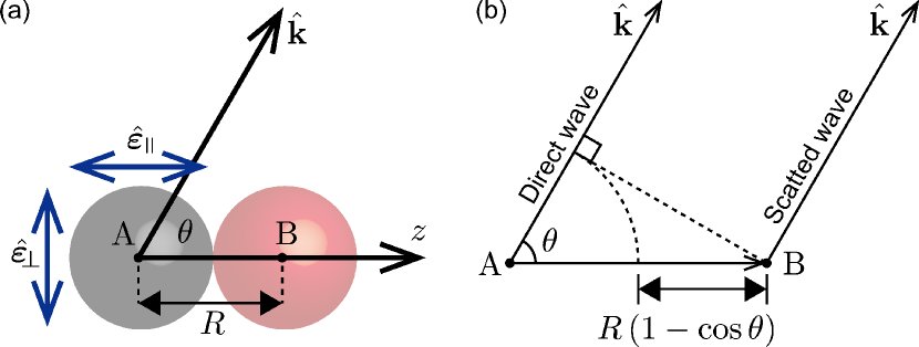
We apply the obtained theoretical model to core-level photoemission from atom A in a heteronuclear diatomic molecule AB in molecular frame, where the molecular axis vector $\mathbf{R}$($\equiv\mathbf{R}_{\mathrm{BA}}$) is parallel to $z$-axis and $\hat{\mathbf{R}}\cdot\hat{\mathbf{k}}=\cos\theta$ (see figure 1 (a)), by a linearly polarized x-ray. We consider two cases that the polarization vector is parallel, $\hat{\mbox{\boldmath$\varepsilon$}}_{\parallel}$, and perpendicular, $\hat{\mbox{\boldmath$\varepsilon$}}_{\perp}$, to $\hat{\mathbf{R}}$. Under the electric dipole approximation, the angular distributions of the direct wave excited with $\hat{\mbox{\boldmath$\varepsilon$}}_{\parallel}$ and $\hat{\mbox{\boldmath$\varepsilon$}}_{\perp}$ are proportional to $\cos\theta$ and $\sin\theta$, respectively.

In the case of $\hat{\mbox{\boldmath$\varepsilon$}}_{\perp}$, we obtain the following simple relations,

	$\displaystyle t\,(\mathbf{k},\hat{\mbox{\boldmath$\varepsilon$}}_{\perp})=t_{\mathrm{abs}}(k)\,,$		(18)
	$\displaystyle t_{\mathrm{path}}(\mathbf{k},\hat{\mbox{\boldmath$\varepsilon$}}_{\perp})=t_{\mathrm{sc}}(\mathbf{k},\hat{\mbox{\boldmath$\varepsilon$}}_{\perp})=0\,.$		(19)

These relations reflect the following physical mechanism: since photoelectrons are not emitted in the direction of atom B, no photoelectrons are scattered by atom B. As a consequence, only photoelectrons directly emitted from atom A are observed. Therefore, the molecule-specific time delays $t_{\mathrm{path}}(\mathbf{k},\hat{\mbox{\boldmath$\varepsilon$}}_{\perp})$ and $t_{\mathrm{sc}}(\mathbf{k},\hat{\mbox{\boldmath$\varepsilon$}}_{\perp})$ become zero, and $t\,(\mathbf{k},\hat{\mbox{\boldmath$\varepsilon$}}_{\perp})$ is reduced to the core-level photoemission delay of a single atom A.

To consider the case of $\hat{\mbox{\boldmath$\varepsilon$}}_{\parallel}$, we employ the single scattering approximation which takes into account up to the second term in equation (8): $\tau\sim T+TGT$. This works in the high energy limit ($\gtrsim 100$ eV). According to this theoretical model, the continuum state is the superposition of the direct wave from atom A and the single scattered wave at B after propagation from A to B. These two waves correspond to the first and second terms in equation (10), respectively. Thus, we obtain a compact form for $t_{\mathrm{path}}^{(1)}(k,\theta)$,

$\displaystyle t_{\mathrm{path}}^{(1)}(k,\theta)=\frac{1}{2}\frac{R\left(1-\cos\theta\right)}{k}\times\frac{1}{2}\left(1-\frac{\cos^{2}\theta-\displaystyle{\frac{1}{R^{2}}}\left|f^{\mathrm{B}}(k,\theta)\right|^{2}}{J^{\,\mathrm{A}\,(1)}(k,\theta)}\right)$

and

		$\displaystyle J^{\,\mathrm{A}\,(1)}(k,\theta)=\cos^{2}\theta+\frac{1}{R^{2}}\left|f^{\mathrm{B}}(k,\theta)\right|^{2}$
		$\displaystyle+2\cos\theta\,\frac{1}{R}\left|f^{\mathrm{B}}(k,\theta)\right|\cos\left[kR\left(1-\cos\theta\right)+\mathrm{arg}\left\{f^{\mathrm{B}}(k,\theta)\right\}\right]~{},$

where the superscript $(1)$ indicates the scattering order and $J^{\,\mathrm{A}\,(1)}(k,\theta)$ is a first order approximation of equation (17) multiplied by $\left|T_{1}^{\mathrm{A}}\right|^{2}k/\pi$. Hereafter, we rewrite the argument $(\mathbf{k},\hat{\mbox{\boldmath$\varepsilon$}}_{\parallel})$ as $(k,\theta)$. $t_{\mathrm{path}}^{(1)}(k,\theta)$ can be interpreted as follows: the factor $R\left(1-\cos\theta\right)/k$ is a travelling time over a distance $R\left(1-\cos\theta\right)$, which is the difference of pathway to the detector between the single scattering wave and free-electron wave (see figure 1(b)). The rest of the terms are responsible for the oscillational structure (oscillating with $kR\left(1-\cos\theta\right)$) due to the interference between the direct and scattered waves.

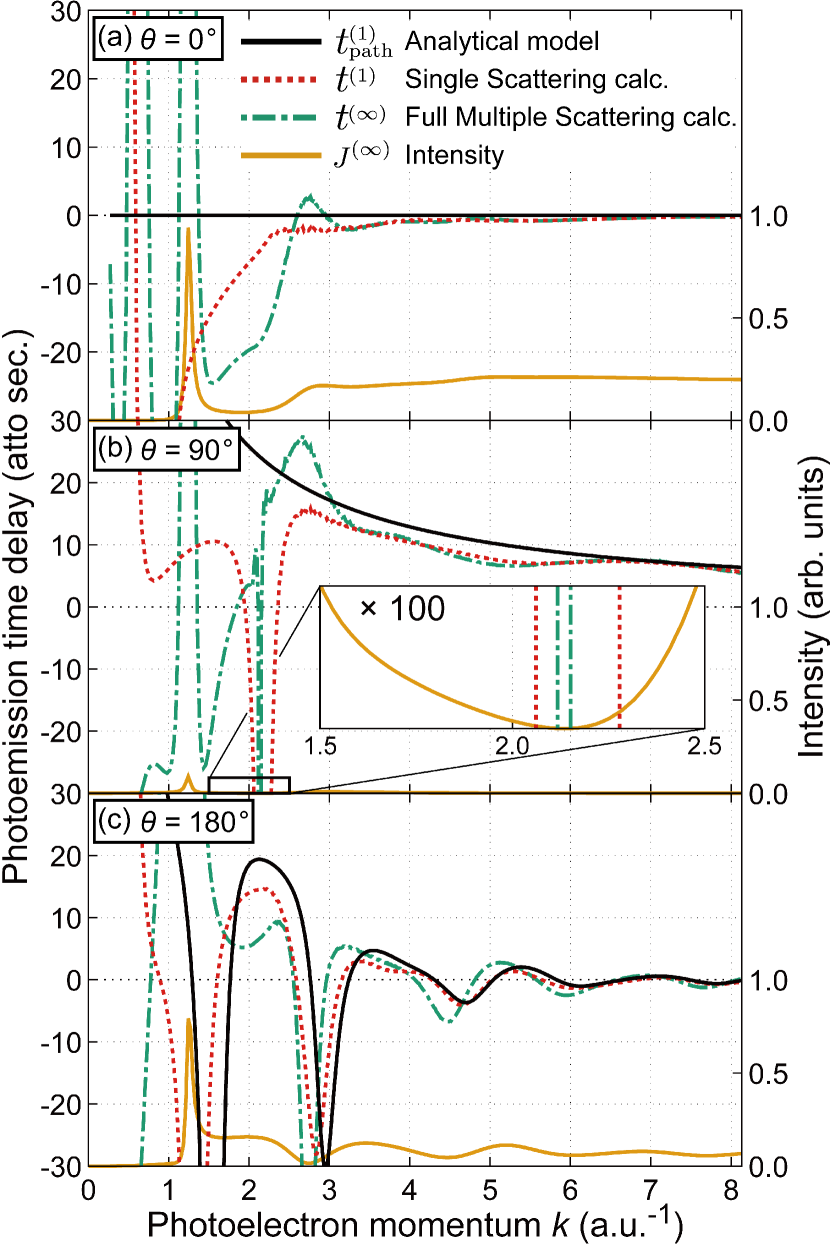
We further investigated the photoemission time delay in the molecular frame, using a specific example, i.e. C 1$s$ core-level photoionization in CO. Since the time delay due to the potential rapidly decreases with the increase in the photoelectron energy, in the high energy regime we expect that $t_{\mathrm{path}}$ ($\sim t^{(1)}_{\mathrm{path}}$) plays a substantial role in equation (13). To verify this, we compared $t^{(1)}_{\mathrm{path}}(k,\theta)$ against more precise forms, i.e. $t^{(\infty)}(k,\theta)$, which is $t(k,\theta)$ considered for the full multiple scattering process, and $t^{(1)}(k,\theta)$ which is its single scattering approximation form (see figure 2). The calculations for $t^{(1)}(k,\theta)$ and $t^{(\infty)}(k,\theta)$ were performed using the multiple scattering program MsSpec [35], taking account of all three terms in equation (13). In figure 2, we see that $t^{(\infty)}(k,\theta)$ converges to $t^{(1)}(k,\theta)$ with increase in energy and both approach $t^{(1)}_{\mathrm{path}}(k,\theta)$ in the high energy region ($k\,\,\gtrsim\,\,3.5\,\,\mathrm{a.u.}^{-1}$) at all angles. Thus, understanding the behaviour of $t^{(1)}_{\mathrm{path}}(k,\theta)$ helps us to have some insight into the core-level photoemission time delay.

In the low energy region, full multiple scattering (infinite order scattering) should be taken into account. We see that $t^{(\infty)}(k,\theta)$ diverges to positive values at about $k=1.24$ a.u.^-1 for each angle in figure 2. This energy position corresponds to the shape resonance energy, which can be confirmed by the peak position of the intensity in equation (17) $J^{(\infty)}(k,\theta)$ calculated with full multiple scattering method. This large time delay indicates that the photoelectrons are trapped by resonance states originating from the molecular structure. Although muffin-tin approximation does not work well in the low energy region for highly anisotropic systems such as linear molecules, it is helpful for qualitative understanding of physics. Another specific phenomenon is that when the intensity becomes zero at $k=0.61$, 2.13 and 2.75 for $\theta=0^{\circ}$, 90^∘ and 180^∘, respectively, the photoemission time delay becomes large. It can be understood that this divergence is due to the intensity in the denominator getting to zero in equations (15) and (16).

Let us look into the details of angular dependence of $t^{(1)}_{\mathrm{path}}(k,\theta)$, especially for some specific angles $0^{\circ}$, $90^{\circ}$ and $180^{\circ}$. At $\theta=0^{\circ}$,

$$t^{(1)}_{\mathrm{path}}(k,0)=0.$$

(22)

As we see, there is no delay caused. This is because the single scattering wave follows the same photoemission pathway as the free electron wave. Thus this equation justifies that the core-level photoemission time delay measured at $\theta=0^{\circ}$ in the high-energy region can be treated as a reference for the measurement. At $\theta=90^{\circ}$,

$\displaystyle t_{\mathrm{path}}^{(1)}\left(k,\frac{\pi}{2}\right)=\frac{1}{2}\frac{R}{k}\,.$

(23)

We notice that this is just the travelling time of the photoelectron from atom A to B, so that this relation may be used as a probe of the bondlength of a heteronuclear diatomic molecule. This can be explained by the following simple considerations. Since $\theta=90^{\circ}$ is the forbidden angle for direct wave (remember now $\hat{\mbox{\boldmath$\varepsilon$}}_{\parallel}$) under the electric dipole approximation, the detected photoelectron must be scattered by the surrounded atom after propagation from A to B. Thus, the time delay is caused by the propagation. At $\theta=180^{\circ}$, $t_{\mathrm{path}}^{(1)}$ oscillates with frequency $2R$ according to equation (A multiple scattering theoretical approach to time delay in high energy core-level photoemission of heteronuclear diatomic molecules). The oscillatory structure is practically the same in origin as the extended x-ray absorption fine structure (EXAFS) and is caused by the interference between the direct photoelectron wave and the scattered wave. Thus it also includes the structural information.

In conclusion, we first derived expressions of core-level photoemission time delay using multiple scattering theory in equations (14)-(17). These equations work for any kind of system, not only molecules but also 2D and 3D extended systems. We applied our theoretical model to heteronuclear diatomic molecules in the high-energy region. The results revealed the angular dependence of the photoemission time delay in the molecular frame and provided a physical interpretation of the photoemission time delay caused by the molecular structure, which is not present in the photoemission time delay of a single atom. In particular, the photoemission time delay observed in the direction perpendicular to the molecular axis set to parallel to the polarization axis can be interpreted as the travelling time spent by photoelectron to propagate between two atoms. This feature indicates that the measurement of core-level photoemission time delay can be a probe not only for dynamics of molecular photoionization (i.e. photoelectron scattering by the anisotropic molecular potential) but also for structural dynamics, e.g. for structural changes of molecules photo-excited by the ultraviolet laser. Further extension of this work will provide a new probe for the electronic and structural dynamics of polyatomic molecules, clusters and materials in the solid and liquid phases.

References

- [1] A. L. Cavalieri, N. Müller, Th. Uphues, V. S. Yakovlev, A. Baltuška, B. Horvath, B. Schmidt, L. Blümel, R. Holzwarth, S. Hendel, M. Drescher, U. Kleineberg, P. M. Echenique, R. Kienberger, F. Krausz, and U. Heinzmann. Attosecond spectroscopy in condensed matter. Nature, 449(7165):1029–1032, October 2007.
- [2] M. Schultze, M. Fiess, N. Karpowicz, J. Gagnon, M. Korbman, M. Hofstetter, S. Neppl, A. L. Cavalieri, Y. Komninos, T. Mercouris, C. A. Nicolaides, R. Pazourek, S. Nagele, J. Feist, J. Burgdorfer, A. M. Azzeer, R. Ernstorfer, R. Kienberger, U. Kleineberg, E. Goulielmakis, F. Krausz, and V. S. Yakovlev. Delay in photoemission. Science, 328(5986):1658–1662, June 2010.
- [3] Renate Pazourek, Stefan Nagele, and Joachim Burgdörfer. Attosecond chronoscopy of photoemission. Reviews of Modern Physics, 87(3):765–802, August 2015.
- [4] P. M. Paul, E. S. Toma, P. Breger, G. Mullot, F. Augé, Ph. Balcou, H. G. Muller, and P. Agostini. Observation of a train of attosecond pulses from high harmonic generation. Science, 292(5522):1689–1692, June 2001.
- [5] J M Dahlström, A L’Huillier, and A Maquet. Introduction to attosecond delays in photoionization. Journal of Physics B: Atomic, Molecular and Optical Physics, 45(18):183001, August 2012.
- [6] M. Isinger, R. J. Squibb, D. Busto, S. Zhong, A. Harth, D. Kroon, S. Nandi, C. L. Arnold, M. Miranda, J. M. Dahlström, E. Lindroth, R. Feifel, M. Gisselbrecht, and A. L’Huillier. Photoionization in the time and frequency domain. Science, 358(6365):893–896, November 2017.
- [7] Jasper Peschel, David Busto, Marius Plach, Mattias Bertolino, Maria Hoflund, Sylvain Maclot, Jimmy Vinbladh, Hampus Wikmark, Felipe Zapata, Eva Lindroth, Mathieu Gisselbrecht, Jan Marcus Dahlström, Anne L’Huillier, and Per Eng-Johnsson. Complete characterization of multi-channel single photon ionization, 2021.
- [8] Martin Huppert, Inga Jordan, Denitsa Baykusheva, Aaron von Conta, and Hans Jakob Wörner. Attosecond delays in molecular photoionization. Physical Review Letters, 117(9), August 2016.
- [9] S. Beaulieu, A. Comby, A. Clergerie, J. Caillat, D. Descamps, N. Dudovich, B. Fabre, R. Géneaux, F. Légaré, S. Petit, B. Pons, G. Porat, T. Ruchon, R. Taïeb, V. Blanchet, and Y. Mairesse. Attosecond-resolved photoionization of chiral molecules. Science, 358(6368):1288–1294, December 2017.
- [10] J. Vos, L. Cattaneo, S. Patchkovskii, T. Zimmermann, C. Cirelli, M. Lucchini, A. Kheifets, A. S. Landsman, and U. Keller. Orientation-dependent stereo Wigner time delay and electron localization in a small molecule. Science, 360(6395):1326–1330, June 2018.
- [11] S. Nandi, E. Plésiat, S. Zhong, A. Palacios, D. Busto, M. Isinger, L. Neoričić, C. L. Arnold, R. J. Squibb, R. Feifel, P. Decleva, A. L’Huillier, F. Martín, and M. Gisselbrecht. Attosecond timing of electron emission from a molecular shape resonance. Science Advances, 6(31):eaba7762, July 2020.
- [12] Shubhadeep Biswas, Benjamin Förg, Lisa Ortmann, Johannes Schötz, Wolfgang Schweinberger, Tomáš Zimmermann, Liangwen Pi, Denitsa Baykusheva, Hafiz A. Masood, Ioannis Liontos, Amgad M. Kamal, Nora G. Kling, Abdullah F. Alharbi, Meshaal Alharbi, Abdallah M. Azzeer, Gregor Hartmann, Hans J. Wörner, Alexandra S. Landsman, and Matthias F. Kling. Probing molecular environment through photoemission delays. Nature Physics, 16(7):778–783, May 2020.
- [13] Xiaochun Gong, Wenyu Jiang, Jihong Tong, Junjie Qiang, Peifen Lu, Hongcheng Ni, Robert Lucchese, Kiyoshi Ueda, and Jian Wu. Asymmetric attosecond photoionization in molecular shape resonance. Physical Review X, 12(1), January 2022.
- [14] Saijoscha Heck, Denitsa Baykusheva, Meng Han, Jia-Bao Ji, Conaill Perry, Xiaochun Gong, and Hans Jakob Wörner. Attosecond interferometry of shape resonances in the recoil frame of CF 4. Science Advances, 7(49), December 2021.
- [15] Xiaochun Gong, Saijoscha Heck, Denis Jelovina, Conaill Perry, Kristina Zinchenko, and Hans Jakob Wörner. Attosecond spectroscopy of size-resolved water clusters, 2021.
- [16] Zhensheng Tao, Cong Chen, Tibor Szilvási, Mark Keller, Manos Mavrikakis, Henry Kapteyn, and Margaret Murnane. Direct time-domain observation of attosecond final-state lifetimes in photoemission from solids. Science, 353(6294):62–67, July 2016.
- [17] M. Lucchini, S. A. Sato, A. Ludwig, J. Herrmann, M. Volkov, L. Kasmi, Y. Shinohara, K. Yabana, L. Gallmann, and U. Keller. Attosecond dynamical franz-keldysh effect in polycrystalline diamond. Science, 353(6302):916–919, August 2016.
- [18] M. Ossiander, J. Riemensberger, S. Neppl, M. Mittermair, M. Schäffer, A. Duensing, M. S. Wagner, R. Heider, M. Wurzer, M. Gerl, M. Schnitzenbaumer, J. V. Barth, F. Libisch, C. Lemell, J. Burgdörfer, P. Feulner, and R. Kienberger. Absolute timing of the photoelectric effect. Nature, 561(7723):374–377, September 2018.
- [19] Inga Jordan, Martin Huppert, Dominik Rattenbacher, Michael Peper, Denis Jelovina, Conaill Perry, Aaron von Conta, Axel Schild, and Hans Jakob Wörner. Attosecond spectroscopy of liquid water. Science, 369(6506):974–979, August 2020.
- [20] Yoann Pertot, Cédric Schmidt, Mary Matthews, Adrien Chauvet, Martin Huppert, Vit Svoboda, Aaron von Conta, Andres Tehlar, Denitsa Baykusheva, Jean-Pierre Wolf, and Hans Jakob Wörner. Time-resolved x-ray absorption spectroscopy with a water window high-harmonic source. Science, 355(6322):264–267, January 2017.
- [21] Seth L. Cousin, Nicola Di Palo, Bárbara Buades, Stephan M. Teichmann, M. Reduzzi, M. Devetta, A. Kheifets, G. Sansone, and Jens Biegert. Attosecond streaking in the water window: A new regime of attosecond pulse characterization. Physical Review X, 7(4), November 2017.
- [22] Nariyuki Saito, Hiroki Sannohe, Nobuhisa Ishii, Teruto Kanai, Nobuhiro Kosugi, Yi Wu, Andrew Chew, Seunghwoi Han, Zenghu Chang, and Jiro Itatani. Real-time observation of electronic, vibrational, and rotational dynamics in nitric oxide with attosecond soft x-ray pulses at 400 eV. Optica, 6(12):1542, December 2019.
- [23] Joseph Duris, Siqi Li, Taran Driver, Elio G. Champenois, James P. MacArthur, Alberto A. Lutman, Zhen Zhang, Philipp Rosenberger, Jeff W. Aldrich, Ryan Coffee, Giacomo Coslovich, Franz-Josef Decker, James M. Glownia, Gregor Hartmann, Wolfram Helml, Andrei Kamalov, Jonas Knurr, Jacek Krzywinski, Ming-Fu Lin, Jon P. Marangos, Megan Nantel, Adi Natan, Jordan T. O’Neal, Niranjan Shivaram, Peter Walter, Anna Li Wang, James J. Welch, Thomas J. A. Wolf, Joseph Z. Xu, Matthias F. Kling, Philip H. Bucksbaum, Alexander Zholents, Zhirong Huang, James P. Cryan, and Agostino Marinelli. Tunable isolated attosecond x-ray pulses with gigawatt peak power from a free-electron laser. Nature Photonics, 14(1):30–36, December 2019.
- [24] F. Holzmeier, J. Joseph, J. C. Houver, M. Lebech, D. Dowek, and R. R. Lucchese. Influence of shape resonances on the angular dependence of molecular photoionization delays. Nature Communications, 12(1), December 2021.
- [25] Jonas Rist, Kim Klyssek, Nikolay M. Novikovskiy, Max Kircher, Isabel Vela-Pérez, Daniel Trabert, Sven Grundmann, Dimitrios Tsitsonis, Juliane Siebert, Angelina Geyer, Niklas Melzer, Christian Schwarz, Nils Anders, Leon Kaiser, Kilian Fehre, Alexander Hartung, Sebastian Eckart, Lothar Ph. H. Schmidt, Markus S. Schöffler, Vernon T. Davis, Joshua B. Williams, Florian Trinter, Reinhard Dörner, Philipp V. Demekhin, and Till Jahnke. Measuring the photoelectron emission delay in the molecular frame. Nature Communications, 12(1), November 2021.
- [26] Alexis Chacon, Manfred Lein, and Camilo Ruiz. Asymmetry of Wigner’s time delay in a small molecule. Physical Review A, 89(5), May 2014.
- [27] P Hockett, E Frumker, D M Villeneuve, and P B Corkum. Time delay in molecular photoionization. Journal of Physics B: Atomic, Molecular and Optical Physics, 49(9):095602, April 2016.
- [28] Denitsa Baykusheva and Hans Jakob Wörner. Theory of attosecond delays in molecular photoionization. The Journal of Chemical Physics, 146(12):124306, March 2017.
- [29] Bejan Ghomashi, Nicolas Douguet, and Luca Argenti. Attosecond intramolecular scattering and vibronic delays. Phys. Rev. Lett., 127:203201, Nov 2021.
- [30] Keisuke Hatada, Kuniko Hayakawa, Maurizio Benfatto, and Calogero R Natoli. Full-potential multiple scattering theory with space-filling cells for bound and continuum states. Journal of Physics: Condensed Matter, 22(18):185501, April 2010.
- [31] C. R. Natoli, M. Benfatto, S. Della Longa, and K. Hatada. X-ray absorption spectroscopy: state-of-the-art analysis. Journal of Synchrotron Radiation, 10(1):26–42, Jan 2003.
- [32] Marvin L Goldberger and Kenneth M Watson. Collision theory. Courier Corporation, 2004.
- [33] F Ota, K Yamazaki, D Sébilleau, K Ueda, and K Hatada. Theory of polarization-averaged core-level molecular-frame photoelectron angular distributions: I. a full-potential method and its application to dissociating carbon monoxide dication. Journal of Physics B: Atomic, Molecular and Optical Physics, 54(2):024003, January 2021.
- [34] J. J. Rehr, R. C. Albers, C. R. Natoli, and E. A. Stern. New high-energy approximation for x-ray-absorption near-edge structure. Physical Review B, 34(6):4350–4353, September 1986.
- [35] Didier Sébilleau, Calogero Natoli, George M Gavaza, Haifeng Zhao, Fabiana Da Pieve, and Keisuke Hatada. Msspec-1.0: A multiple scattering package for electron spectroscopies in material science. Computer Physics Communications, 182(12):2567–2579, 2011.