A multi-shock model for the density variance of anisotropic, highly-magnetised, supersonic turbulence

Log-normal models for the density can be traced back to Vazquez-Semadeni (1994), where they explore different functional forms for the $\rho\,$-PDF in order to model the self-similar, hierarchical structure of density in the cool, pressureless $(\mathcal{M}\gg 1)$, non-self-gravitating ISM regime. Vazquez-Semadeni (1994) considers the density fluctuation random variable, $\delta=\rho/\rho_{0}$, and motivates the log-normal PDF by assuming that for some time, $t_{n}$, the density can be expressed as a multiplicative interaction through independent density fluctuations, hence,

where $\rho(t_{0})$ is the initial density. Under the log-transform, the product becomes a sum,

If each $\delta$ follows the same underlying distribution and are independent from each other (i.e., not correlated) then the central limit theorem states that the distribution of the log-density affected by this additive random process is approximately normal, specifically:

where $\mathcal{N}(0,\sigma_{s}^{2})$ is the normal distribution with mean zero, as $n$, the number of density fluctuations, approaches infinity. This lets us understand the nature of a single density fluctuation changing in time. However, Vazquez-Semadeni (1994) further argues that since the hydrodynamical equations are self-similar in space (i.e., invariant under arbitrary length scalings), the fluctuations should be log-normal globally. Passot & Vázquez-Semadeni (1998) extend this idea, recasting $\delta$ as a perturbation in the density from a transient shock, rather than just a generic turbulent fluctuation. This means that one could relate the well-known shock-jump relations to the $\sigma_{\rho}$ variable³³3For a log-normally distributed variable, $\rho/\rho_{0}$, the variance of the log-variable obeys $\sigma_{\ln\rho/\rho_{0}}^{2}=\ln(1+\sigma^{2}_{\rho/\rho_{0}})$ and is the value that is commonly reported in the literature. Throughout this study we however consider $\sigma^{2}_{\rho/\rho_{0}}$, without making any assumptions of the underlying distribution., formulating the relation,

As described in §1, the density $\sigma^{2}_{\rho/\rho_{0}}-\mathcal{M}$ relation has been studied intensely over the last two decades. The main idea is that $\sigma^{2}_{\rho/\rho_{0}}$, or the spread of the $\rho$-PDF is a function of the underlying physical processes that govern the fluid, whether it be motivated by the supersonic plasmas of the ISM (e.g Mac Low & Klessen, 2004; Federrath et al., 2008, 2010; Price et al., 2011; Padoan & Nordlund, 2011; Federrath & Klessen, 2012; Ginsburg et al., 2013; Federrath & Banerjee, 2015; Klessen & Glover, 2016) or the subsonic density fluctuations in the hot, stratified, intracluster medium (ICM; e.g. Mohapatra et al. 2020a, b). More specifically, for an isothermal, turbulent, hydrodynamic medium,

where $b$ is controlled by the amount of solenoidal ($\nabla\times\mathrm{{\mn@boldsymbol{\mathit{F}}}}$) and compressive ($\nabla\cdot\mathrm{{\mn@boldsymbol{\mathit{F}}}}$) modes injected by the turbulence driving field $\mathrm{{\mn@boldsymbol{\mathit{F}}}}$ (Federrath et al., 2008, 2010; Price et al., 2011). Introducing a non-isothermal equation of state gives the relation,

where $\gamma$ is the adiabatic index of the medium (Nolan et al., 2015). For isothermal and magnetised turbulence, the variance changes with the correlation between $B$ and $\rho$,

where $\beta_{0}=2\mathcal{M}^{2}_{\text{A0}}/\mathcal{M}^{2}$ is the plasma beta with respect to the mean magnetic field, which was explored in Molina et al. (2012) and will be discussed in more detail in §3.1.

The relation between density contrasts and the volume-weighted variance of the underlying field is given by

where $\operatorname{\mathcal{V}}$ is the volume for the fluid region of interest (Padoan & Nordlund, 2011). Molina et al. (2012) turn Equation 14 into an integral over density contrasts by constructing the function $\operatorname{d}\!{\operatorname{\mathcal{V}}}=f(\rho_{1}/\rho_{0})\operatorname{d}\!{(\rho_{1}/\rho_{0})}$ based on the shock geometry, where $\rho_{1}/\rho_{0}$ is the density contrast for a single shock. Molina et al. (2012) use this to derive an analytical model for $\sigma^{2}_{\rho/\rho_{0}}$ for different $B-\rho$ correlations, assuming that the shock geometry is the same for all shocks in the magnetised plasma, and that there is no preferential direction for the density contrast produced by the shocks, i.e., that they are isotropic. This is a good approximation for $\operatorname{\mathcal{M}_{\text{A0}}}\geq 2$, when the turbulent component of the magnetic field is larger than or equal to the mean-field component (Beattie et al., 2020). However, it breaks down for $\operatorname{\mathcal{M}_{\text{A0}}}\lesssim 1$, i.e., when the mean field is very strong, relevant to this study.

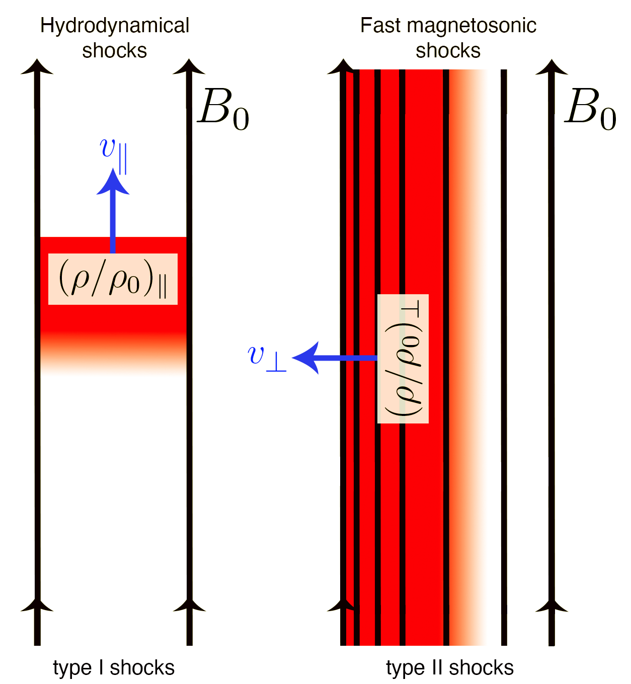
Anisotropic, sub-Alfvénic, compressive density structures were studied in detail in Beattie & Federrath (2020), showing that the anisotropy of the density fluctuations is a function of both $\mathcal{M}$ and $\operatorname{\mathcal{M}_{\text{A0}}}$. They attributed the anisotropy to hydrodynamical shocks that form perpendicular to $\mathrm{{\mn@boldsymbol{\mathit{B}}}}_{0}$, causing parallel fluctuations, and fast magnetosonic waves that form parallel to $\mathrm{{\mn@boldsymbol{\mathit{B}}}}_{0}$, causing perpendicular fluctuations, illustrated schematically in Figure 1. This is consistent with findings from Tritsis & Tassis (2016), who showed that observations of striations (density perturbations that form parallel to $\mathrm{{\mn@boldsymbol{\mathit{B}}}}_{0}$ in sub-Alfvénic flows) are reproducible when one considers fast magnetosonic wave perturbations. In this study, we take this phenomenology further and model the variance of density structures arising from a supersonic velocity field with a strong magnetic guide field, considering these two types of shocks.

The general form of this variance can be constructed as follows⁴⁴4By expressing the variance as we have below we are assuming that the density fluctuations are symmetric around the magnetic field. This was shown explicitly through the elliptic symmetry with respect to the magnetic field of the 2D density power spectra in Figure 2 of Beattie & Federrath (2020) and 2D structure functions in Hu et al. (2020).,

which decomposes the total variance into components of the density variance parallel to $\mathrm{{\mn@boldsymbol{\mathit{B}}}}_{0}$, termed $\sigma^{2}_{\rho/\rho_{0}\parallel}$, and perpendicular to $\mathrm{{\mn@boldsymbol{\mathit{B}}}}_{0}$, termed $\sigma^{2}_{\rho/\rho_{0}\perp}$. By assuming that these fluctuations are independent from one another we can further simplify the equation to

where the correlation term, $2\sigma_{\rho/\rho_{0}\parallel}\sigma_{\rho/\rho_{0}\perp}$, between the fluctuations becomes zero in the statistical average⁵⁵5This is a justified assumption because the statistically-averaged elliptic power spectra in Figure 2 of Beattie & Federrath (2020) do not show any rotations in the $k_{\perp}-k_{\parallel}$ plane, i.e. the principal axes of the ellipses fitted to the power spectra are aligned with the $k_{\perp}-k_{\parallel}$ coordinate axis, where $k_{\perp}$ corresponds to wave numbers perpendicular to $\mathrm{{\mn@boldsymbol{\mathit{B}}}}_{0}$ and $k_{\parallel}$ for parallel wave numbers. This means that the density fluctuations along and across the mean field are statistically independent from each other, and hence $2\sigma_{\rho/\rho_{0}\parallel}\sigma_{\rho/\rho_{0}\perp}\approx 0$.. For a short discussion on how the velocity and magnetic field is arranged in this turbulence regime we refer the reader to Appendix A. The main purpose of this study is therefore to explore and model each of these components, extending the work of Molina et al. (2012) and Beattie & Federrath (2020) and indeed the numerous works on $\sigma^{2}_{\rho/\rho_{0}}$, into the sub-Alfvénic, anisotropic, supersonic turbulent regime. Furthermore, with the development of a density fluctuation model, this is the first step towards an anisotropic, magneto-turbulent star formation theory.

Consider a planar shock with surface area $\ell^{2}_{\rm shock}$ and shock width $\lambda$, propagating in a system with volume $\mathcal{V}=L^{3}$. The volume of the shock is then

The shock width is proportional to the density jump between the pre-shock ($\rho_{0}$) and post-shock ($\rho_{1}$) densities, multiplied by the integral scale of the turbulence, $\theta L$, i.e., the scale where velocity structure is no longer correlated,

which is derived in Padoan & Nordlund (2011) by balancing the ram and thermal pressures for a shock in hydrodynamical turbulence. We substitute Equation 18 into 17 to reveal the volume of the shock in terms of the density contrast,

Now assuming that $\operatorname{d}\!{\operatorname{\mathcal{V}}}\approx\operatorname{d}\!{\operatorname{\mathcal{V}}_{\text{shock}}}$ we can construct the volume differential, substitute it into Equation 14 and integrate it to construct the variance as a function of density contrasts. Hence,⁶⁶6We consider the transformation $\operatorname{d}\!{\operatorname{\mathcal{V}}}=|\frac{\operatorname{d}\!{\operatorname{\mathcal{V}}}}{\operatorname{d}\!{(}\rho_{1}/\rho_{0})}|\operatorname{d}\!{(}\rho_{1}/\rho_{0})$ to simplify the treatment of the limits in Equation 21.

and therefore we can rewrite Equation 14 in terms of density contrasts between $1\leq\rho_{1}/\rho_{0}\leq\rho/\rho_{0}$⁷⁷7Note that we integrate $\rho_{1}/\rho_{0}$ from 1, i.e., when the pre- and post-shock densities are the same, up to an arbitrarily large density contrast, $\rho/\rho_{0}$. This is the range of density contrasts where a shock is well defined., which is the density domain for which shocks are well-defined in,

where $\operatorname{\mathcal{V}}=L^{3}$ cancels between the differential element of the shock and volume-weighted integral. What this means is that for a single-shock model we average over the shock-jump conditions through the whole volume of interest. This will be important for generalising this model to multiple shocks in §3.3. The first term in Equation 23, $\rho/\rho_{0}$, the over-densities, dominates the total variance, since the amplitude of the density fluctuations is large in supersonic turbulence. Both $\rho_{0}/\rho$, the under-densities, and $\ln(\rho/\rho_{0})$, the logarithmic over-densities are small in comparison, allowing us to approximate the total variance as solely dependent upon the over-densities (Padoan & Nordlund, 2011). Assuming the integral scale factor is $\theta\approx 1$, i.e., of order the system scale (Federrath & Klessen, 2012), and making the above approximation we find the relation,

which is the key result that Padoan & Nordlund (2011) and Molina et al. (2012) use to relate the variance to the shock-jump conditions. Before generalising this result, we first consider the details of the two shock types that we use to construct our model of the anisotropic density variance.

We have now seen that the variance of a stochastic density field full of shocks can be related to the shock-jump conditions. The shock-jump conditions can be derived in the regular Rankine-Hugoniot fashion, where we equate the upstream and downstream $\mathrm{{\mn@boldsymbol{\mathit{B}}}}$, $\rho\mathrm{{\mn@boldsymbol{\mathit{v}}}}$ and $\rho$ (for an isothermal shock) across the shock boundary, in the local frame of the shock, to conserve energy, momentum and mass (Landau & Lifshitz, 1959), and we follow Molina et al. (2012) to include the magnetic pressure contribution in the derivation. In the following two subsections we will describe two different types of shocks that are derived using this method.

Now we combine Equation 26 and Equation 29 to model the total variance of the anisotropic density field, i.e., we assume the stochastic medium of interest is composed out of the type I and type II shocks discussed above. Thus, we model the total fluctuations as the sum of integrals over the shock-jump conditions in the parallel and perpendicular directions, as discussed in §3.1, assuming that the fluctuations are independent from one another. In reality there will be some non-linear mixing of the shocks (e.g., type II shocks compressing the type I shocks longitudinally, changing the shock jump conditions through a multiplicative interaction) and, in principle, a larger diversity of shocks and density fluctuations, but we adopt the most parsimonious anisotropic model for the variance that one can formulate and leave generalisations of the model for future studies. The $N$-shock model would sum over $N$ types of uncorrelated shocks with shock-jump conditions $\left(\rho/\rho_{0}\right)_{i}$ and shock volumes $\operatorname{\mathcal{V}}_{i}$, given by

For our two-shock model ($N=2$, for type I and type II), this leads to

Here we describe the numerical data that we use to test our density variance model. These are high-resolution, three-dimensional, ideal magnetohydrodynamical (MHD) simulations of supersonic turbulence. The ideal, isothermal MHD equations are

where $\mathrm{{\mn@boldsymbol{\mathit{v}}}}$ is the fluid velocity, $\rho$ the density, $\mathrm{{\mn@boldsymbol{\mathit{B}}}}$ the magnetic field, $c_{s}$ the sound speed and $\mathrm{{\mn@boldsymbol{\mathit{F}}}}$, a stochastic function that drives the turbulence. We use a modified version of flash based on version 4.0.1 (Fryxell et al., 2000; Dubey et al., 2008) to solve the MHD equations in a periodic box with dimensions $L^{3}$, on a uniform grid with resolution $512^{3}$, using the multi-wave, approximate Riemann solver framework described in Bouchut et al. (2010) and implemented in flash by Waagan et al. (2011). For a detailed discussion of the simulations we refer the reader to Beattie & Federrath (2020) and Beattie et al. (2020). Table 1 provides a summary of the important time-averaged parameter values. Here we briefly summarise the key methods and properties of the simulations.

The initial velocity field is set to $\mathrm{{\mn@boldsymbol{\mathit{v}}}}(x,y,z,t=0)=\mathrm{{\mn@boldsymbol{\mathit{0}}}}$, with units $c_{s}=1$, and the density field $\rho(x,y,z,t=0)=\rho_{0}$, with units $\rho_{0}=1$. The turbulent acceleration field, $\mathrm{{\mn@boldsymbol{\mathit{F}}}}$, in Equation 34 follows an Ornstein-Uhlenbeck process in time and is constructed such that we can control the mixture of solenoidal and compressive modes in $\mathrm{{\mn@boldsymbol{\mathit{F}}}}$ (see Federrath et al. 2008; Federrath et al. 2009; Federrath et al. 2010 for a detailed discussion of the turbulence driving). We choose to drive with a natural mixture of the two modes (Federrath et al., 2010), which corresponds to $b\approx 0.4$. We isotropically drive in wavenumber space, centred on $k=2$, corresponding to real-space scales of $\ell_{D}=L/2$, and falling off to zero with a parabolic spectrum between $k=1$ and $k=3$. Thus, energy is injected only on large scales and the turbulence on smaller scales develops self-consistently through the MHD equations. The auto-correlation timescale of $\mathrm{{\mn@boldsymbol{\mathit{F}}}}$ is equal to

We vary the sonic Mach number between $\mathcal{M}=2$ and 20, encapsulating the range of observed $\mathcal{M}$ values for turbulent MCs (e.g., Schneider et al. 2013; Federrath et al. 2016; Orkisz et al. 2017; Beattie et al. 2019b). We run the simulations from $0\leq t/T\leq 10$ and extract 51 time realisations of $\rho(x,y,z)$ over $5\leq t/T\leq 10$ to gather data only when the turbulence is in a statistically stationary state (Federrath et al., 2009; Price & Federrath, 2010). For simulations with a strong guide field, a statistically steady state is reached after about $5T$, while for purely hydrodynamical turbulence and super-Afvénic turbulence, stationarity is already reached after about $2T$. All our results are based on time-averages across these 51 realisations, unless explicitly indicated otherwise.

In Figure 4 we show the time-averaged logarithmic density PDFs for the $\operatorname{\mathcal{M}_{\text{A0}}}=0.1$ simulations shown in Table 1. We show a log-normal model fit to the density fluctuations with dotted lines. The density PDFs show that the fluctuations are well described by a log-normal model, especially as $\mathcal{M}$ increases. This is in contrast with hydrodynamical and super-Alfvénic compressible turbulent flows, which become less log-normal as the $\mathcal{M}$ increases (Federrath et al., 2010; Hopkins, 2013b; Mocz & Burkhart, 2019). We leave the detailed analysis of the Gaussianity of the density PDFs for a follow-up study, but stress that in the sub-Alfvénic regime the variance of the density field, which is the focus of this study, is an informative statistic because of the log-normal fluctuations.

In Figure 2 we show density slices through a plane perpendicular to the direction of $\mathrm{{\mn@boldsymbol{\mathit{B}}}}_{0}$, indicated in the top-left plot. The plots are organised such that the top-left plot has the weakest (but still supersonic) turbulence ($\mathcal{M}=2$) and strongest $B_{0}$ ($\operatorname{\mathcal{M}_{\text{A0}}}=0.1$), and the bottom-right plot has the strongest turbulence ($\mathcal{M}=20$) and weakest $B_{0}$ ($\operatorname{\mathcal{M}_{\text{A0}}}=1.0$). The slices reveal the highly-anisotropic density structures that form in sub-Alfvénic, supersonic turbulence. Over-densities and rarefactions from fast magnetosonic shocks (type II shocks) cause ripples through the density running parallel to the magnetic field. The largest density contrasts are from the shocks that form along the magnetic field (type I shocks), which compress the gas density into sharp, fractal filaments. The filamentary structures become less space-filling as $\mathcal{M}$ increases, extending across $\propto L/\mathcal{M}^{2}\propto L/4$ for $\mathcal{M}\approx 2$, to a tiny fraction of the box at $\mathcal{M}\approx 20$, qualitatively consistent with the shock-width model discussed in §3.1.

Using the ospray ray-tracer in visit (Childs et al., 2012) we show examples of the volumetric density field for the M2MA0.1 and M20MA0.1 simulations in Figure 3. Large-scale vortices are revealed in the M2MA0.1 simulation, with sheets of density wrapped around in the direction of the $\mathrm{{\mn@boldsymbol{\mathit{B}}}}_{0}$. The vortices form at roughly the driving scale ($L/2$) of the simulation. The volumetric rendering for M20MA0.1 shows much more small-scale structure compared to M2MA0.1, both along and perpendicular to the direction of $\mathrm{{\mn@boldsymbol{\mathit{B}}}}_{0}$. The large-scale vortices found in M2MA0.1 are roughly at the same scale as the vortices in M20MA0.1, suggesting that it is the driving scale that sets the size of the vortices. Dense, shocked material is compressed along the magnetic field lines, creating the filamentary structures that were found in the slices, oriented perpendicular to the field.

The initial magnetic field, $\mathrm{{\mn@boldsymbol{\mathit{B}}}}(x,y,z)=B_{0}\hat{\mathrm{{\mn@boldsymbol{\mathit{z}}}}}$ at $t=0$, in Equations (34–36) is a uniform field with field lines threaded through the $\hat{\mathrm{{\mn@boldsymbol{\mathit{z}}}}}$ direction of the simulations. $B_{0}$ is set to ensure the desired $\operatorname{\mathcal{M}_{\text{A0}}}$, using the definition of the Alfvén velocity (see footnote 1) and the turbulent Mach number (see Equation 5),

with $B_{0}$ constant in space and time. We set $\operatorname{\mathcal{M}_{\text{A0}}}=0.1,0.5$ and $1.0$ for different simulations (see Table 1), ensuring that the turbulence is in an anisotropic regime (Beattie et al., 2020; Beattie & Federrath, 2020). The total magnetic field is given by

where the fluctuating component of the field, $\delta\mathrm{{\mn@boldsymbol{\mathit{B}}}}$, evolves self-consistently from the MHD equations, with $\mathrm{\left\langle\delta\mathrm{{\mn@boldsymbol{\mathit{B}}}}\right\rangle}_{t}=0$. From previous experiments in the anisotropic regime discussed throughout this study, $|\delta\mathrm{{\mn@boldsymbol{\mathit{B}}}}|/|\mathrm{{\mn@boldsymbol{\mathit{B}}}}_{0}|\approx 10^{-3}-10^{-2}$ (Federrath, 2016a; Beattie et al., 2020). For this reason $\operatorname{\mathcal{M}_{\text{A}}}\approx\operatorname{\mathcal{M}_{\text{A0}}}$ in this regime, however, we explicitly formulate our models around $\operatorname{\mathcal{M}_{\text{A0}}}$, which is an invariant across different $\mathcal{M}$ simulations.

The fluctuation volume fractions, $f_{\parallel}$ and $f_{\perp}$ in Equation 32, determine the contributions of the parallel and perpendicular fluctuations in our model. These parameters naturally come about from considering multiple terms of a volume-weighted statistic, where the total volume is partitioned into distinct sub-volumes for the parallel and perpendicular fluctuations. The volume-filling fractions can be derived by returning to Equation 17, but instead of using a planar shock, we consider shocks that have a reduced volume-filling factor, $f_{i}$,

where $i\in\left\{\parallel,\perp\right\}$ is the volume-filling factor of the shock, e.g., for $f_{i}=1$ the shock is the planar shock from Equation 17, and for $f_{i}<1$ the shock has a smaller volume than a planar shock, which, could be for example, a tubular, filamentary shock. Considering shocks with a variable volume is an important consideration to make in our two-shock model, because the amount of volume that the fluctuations fill encodes how much they contribute to the variance through the density variance integral, Equation 14. Propagating Equation 40 through Equations 20-24, making the same assumptions but for non-planar shocks, shows that

where $f_{\parallel}$ is the volume-filling fraction of the type I shocks and $f_{\perp}$ is the volume fraction of the type II shocks. Note that the geometry of the volume variable shock propagates through to the total volume fraction of the parallel and perpendicular fluctuations, including the rarefactions. This is because the rarefaction region in the flow will share some of the same geometrical properties as the shock, since the gas density is compressed from the rarefaction into the over-density. However, as we discussed in §3.1, the main contributors to the variance are the over-densities, hence,

and Equation 32 immediately follows by substituting in the appropriate shock-jump conditions. Since the volume-filling fractions are for the total parallel and perpendicular fluctuations we assume that they add to unity,

This means our model is an $N-1$ parameter model, where $N$ is the number of shock types, and more explicitly, a one-parameter model for the two-shock model we describe here.

The volume-filling fractions need not be constants, and indeed, may depend upon both $\mathcal{M}$ and $\operatorname{\mathcal{M}_{\text{A0}}}$. For example, Konstandin et al. (2016), Beattie et al. (2019a) and Beattie et al. (2019b) demonstrate that the global fractal dimension $\operatorname{\mathcal{D}}$, which is a measure of the how the most singular structures in the flow fill space, for supersonic turbulence depends upon $\mathcal{M}$, which varies between 3 (space-filling, low-$\mathcal{M}$) and 1 (filaments and tubular shocks, high-$\mathcal{M}$). This is because the flow is more compressible for higher $\mathcal{M}$, reducing $\operatorname{\mathcal{D}}$, which corresponds to the emergence of highly-compressed structures like one-dimensional filaments. Increasing $\mathcal{M}$ also directly affects the geometry of the shocks in the flow, which can be shown by expressing Equation 18, the shock thickness, in terms of the shock-jump conditions for an isothermal, hydrodynamical shocks in pressure equilibrium with the ambient environment,

This establishes that the shocks become more compressed (thinner), filling less space, as $\mathcal{M}$ increases, which means that a reasonable model for the volume fraction of the parallel fluctuations, which is dominated by type I shocks is $f_{\parallel}\propto\mathcal{M}^{-2}$. However, this only holds for $\mathcal{M}\gg 1$, but not for $\mathcal{M}\sim 1$. Thus, we require a phenomenological function for the volume fraction that describes its dependence on $\mathcal{M}$ for both the trans to supersonic flow regime. We consider the form

which describes a function that tends towards $\sim 1/\mathcal{M}^{2}$ when $\mathcal{M}>\mathcal{M}_{\rm c}\gg 1$ and a constant volume fraction, $f_{0}$, for $\mathcal{M}<\mathcal{M}_{\rm c}$, e.g., in the sub- trans-sonic regime, where the type I shock thickness becomes ill-defined, and linear MHD waves (slow, parallel and fast, perpendicular modes) weakly compress the flow. Here, $\mathcal{M}_{\rm c}$ defines a critical Mach number for the transition between the constant and the $\sim\mathcal{M}^{-2}$ regime. Thus, the parameter $f_{0}$ defines the volume-filling fraction of the parallel fluctuations, in the presence of over-densities formed by slow modes, as discussed in §3.2.1. These are acoustic modes that propagate along the magnetic field in the subsonic regime (Landau & Lifshitz, 1959). Note that since we have assumed $f_{\perp}=1-f_{\parallel}$ we only need to consider a model for $f_{\parallel}$.

The first step to fitting our model is to develop a dataset, ($\mathcal{M}_{i}$,$f_{\parallel,i}$), for the different $\operatorname{\mathcal{M}_{\text{A0}}}$ simulation listed in Table 1. Since, as discussed in § 5.1, our model only has a single parameter, $f_{\parallel}$, we can rearrange Equation 32 and solve analytically⁸⁸8This follows from $\sigma^{2}_{\rho/\rho_{0}}=f_{\parallel}\sigma^{2}_{\rho/\rho_{0}\parallel}+f_{\perp}\sigma^{2}_{\rho/\rho_{0}\perp}=f_{\parallel}\sigma^{2}_{\rho/\rho_{0}\parallel}+(1-f_{\parallel})\sigma^{2}_{\rho/\rho_{0}\perp}$ and then solving for $f_{\parallel}.$,

with the single constraint that $f_{\parallel}\in[0,1]$, since it corresponds to a fraction of the total volume. This allows us to generate a function $f_{\parallel}(\mathcal{M})$ for each simulation. We show this data in Figure 5. We then fit the functional form for $f_{\parallel}(\mathcal{M})$, Equation 46, with parameters $f_{0}$ and $\mathcal{M}_{\rm c}$ using a non-linear least squares fitting routine weighted by $1/\Delta f_{\parallel}^{2}$, where $\Delta f_{\parallel}$ is the uncertainty in $f_{\parallel}$, propagated through Equation 47. We show the fits using the solid lines, coloured by $\operatorname{\mathcal{M}_{\text{A0}}}$.

For each of the datasets, the critical sonic Mach number is $\mathcal{M}_{\rm c}\approx 10$ and the $f_{0}$ parameter varies monotonically between $\approx 0.4$–$0.7$, listed in Table 2. There are two important conclusions to make: (1) magnetised turbulence is significantly saturated with shocks above $\mathcal{M}\approx 10$, and (2) the parallel fluctuations become less confined by the magnetic field, and occupy more of the total volume when the magnetic field is weakened. Accordingly, one should expect that $f_{0}\sim 1.0$ as $\operatorname{\mathcal{M}_{\text{A0}}}\rightarrow\infty$, i.e., when there is no confinement from the magnetic field. This reclaims the hydrodynamical $\sigma_{\rho/\rho_{0}}^{2}-\mathcal{M}$ relation. Regardless of the field strength, the high-$\mathcal{M}$ behaviour is the same between the simulations, which is expected since the shock width, $\lambda\sim\mathcal{M}^{-2}$, encodes how the $(b\mathcal{M})^{2}$ term contributes to the total variance once the fluid is sufficiently shocked. This transition is consistent with what Beattie & Federrath (2020) found, where $\mathcal{M}\approx 4-10$ marked the Mach number for when the anisotropy of the 2D power spectrum revealed a morphology dominated by shocks aligned perpendicular to $\mathrm{{\mn@boldsymbol{\mathit{B}}}}_{0}$. Since we have assumed $f_{\perp}=1-f_{\parallel}$ (Equation 44) as $\mathcal{M}$ grows and the parallel fluctuations occupy less and less of the volume until the perpendicular fluctuations contribute the most to the total volume budget for the fluid.

We show some of the shocked regions for both the parallel and perpendicular fluctuations in the top panels of Figure 6, for $\mathcal{M}\approx 20$ turbulence by taking the divergence along and across $\mathrm{{\mn@boldsymbol{\mathit{B}}}}_{0}$. We also show the corresponding density fluctuations in the bottom two panels, of the Figure, where we highlight the $-\nabla\cdot\mathrm{{\mn@boldsymbol{\mathit{v}}}}>0$ regions. We find that the relative fraction of the volume occupied by type I (left-hand panel) and type II (right-hand panel) shocks is qualitatively consistent with our model, as demonstrated by the regions of high compression quantified by $-\nabla\cdot\mathrm{{\mn@boldsymbol{\mathit{v}}}}>0$ in the top panels, and corresponding density structures coloured in the bottom panels. This Figure is primarily for illustrative purposes of type I and type II shocks and their approximate volume filling fractions.

Let us now consider the limiting behaviour of the density variance in our model. The density variance is summarised as

In the high-$\mathcal{M}$ limit we have

which, like the density contrast caused by type II shocks shown in §3.2.2, is asymptotic to a limit fixed by the magnetic field and turbulent parameters. Ours is the first model to predict such a bound for the total density fluctuations, which is set by the strength of the mean magnetic field, the type of driving, and the volume-filling fraction of subsonic fluctuations travelling along $\mathrm{{\mn@boldsymbol{\mathit{B}}}}_{0}$. This tells us that even in the high-$\mathcal{M}$ limit the turbulent driving parameter influences the spread of the PDF, frozen into the variance at high-$\mathcal{M}$. Interestingly, the limiting behaviour is independent of $\mathcal{M}$, as the effect of increasingly sharp density contrasts ($\mathcal{M}^{2}$) of supersonic hydrodynamical shocks is cancelled out by the reduced volume-filling factor of the parallel fluctuations.

The next limit of interest is the low-$\operatorname{\mathcal{M}_{\text{A0}}}$ limit,

Thus, the parallel component of the variance is retained in this limit. We can interpret this as hydrodynamical fluctuations are able to survive along the magnetic field but are confined in a small volume, $f_{\parallel}\mathcal{V}$, and hence are reduced by the volume-filling fraction, $f_{\parallel}$. This value will be significantly less than 1 for $\mathcal{M}\gg 10$, as measured in §5.2. This is a key distinguishing feature from any of the isotropic magnetised models presented in Equation 13 (Molina et al., 2012). Both of these models result in $\sigma^{2}_{\rho/\rho_{0}}=0$ in this limit.

Finally, in the high-$\operatorname{\mathcal{M}_{\text{A0}}}$ limit, as the turbulence transitions from magnetised to hydrodynamic,

which is the well-known, isotropic, hydrodynamic $\mathcal{M}-\sigma^{2}_{\rho/\rho_{0}}$ relation.

We motivated in §1 that there have been a number of ISM observations (Li & Henning, 2011; Li et al., 2013; Soler et al., 2013; Planck Collaboration et al., 2016a, b; Federrath, 2016b; Cox et al., 2016; Malinen et al., 2016; Tritsis & Tassis, 2016; Soler et al., 2017; Tritsis et al., 2018; Heyer et al., 2020; Pillai et al., 2020) and simulations (Soler & Hennebelle, 2017; Tritsis et al., 2018; Beattie & Federrath, 2020; Seifried et al., 2020; Körtgen & Soler, 2020; Barreto-Mota et al., 2021) that show bimodally distributed density structures with respect to the magnetic field.

For example, recent polarimetric observations of nearby MCs reveal that the alignment of filamentary structures in gas column density derived from Herschel submillimetre observations change with the density: high-density structures ($N_{\rm H_{2}}\propto 10^{23}\,\text{cm}^{-2}$, where $N_{\rm H_{2}}$ is the number density of the molecular gas column density) tend to be oriented perpendicularly to, and low-density ($N_{\rm H_{2}}\propto 10^{22}\,\text{cm}^{-2}$) structures parallel to, the mean magnetic field (Planck Collaboration et al., 2016a; Soler et al., 2017; Tritsis et al., 2018; Heyer et al., 2020; Pillai et al., 2020). Through the analysis of numerical MHD turbulence simulations we have identified some of the physics that causes the bimodal alignment of gas density structures during this density transition. To summarise, the alignment in simulations like ours comes about through an interplay between the divergence (compressibility) and the strain (most likely associated with vortex creation; such as those visualised in Figure 3) in the flow. This has been found in multiple studies of highly-magnetised, compressible plasmas, including those simulations presented in Figure 6, (Soler & Hennebelle, 2017; Beattie & Federrath, 2020; Seifried et al., 2020; Körtgen & Soler, 2020). A different model is developed in Xu et al. (2019). They use the Goldreich & Sridhar (1995) anisotropy theory to model the extent of low-density filaments in the warm, diffuse and sub-sonic ISM. This model is most likely not applicable for the highly-compressible flows in the supersonic, cool and dense molecular clouds, which need not conform to the incompressible Goldreich & Sridhar (1995) theory. The transition occurs with or without the presence of self-gravity, and hence seems to be a MHD phenomena (however, self-gravitating MHD simulations are shown to enhance the density structures that are perpendicular to $\mathrm{{\mn@boldsymbol{\mathit{B}}}}_{0}$, e.g. Soler & Hennebelle 2017; Gómez et al. 2018; Barreto-Mota et al. 2021).

Our two-shock model suggests a simple explanation for this density transition described above, irrespective of the physical processes that create the aligned structures, which is beyond the scope of this study. The shock-jump conditions predict that perpendicularly oriented hydrodynamical shocks formed from material flowing along the magnetic field are at least an order of magnitude larger in density contrast compared to parallel oriented fast magnetosonic shocks, formed through shuffling magnetic field lines. We show this qualitatively in Figure 6, with the density contrasts produced by the shocks visualised in the two bottom panels. Hence, we suggest that the observed transition in the density arises from observing these two distinct types of MHD modes.

A further transition is also now reported at even higher column densities, within the filaments (< 0.1pc) themselves (Pillai et al., 2020). Inside of the filaments gravity-induced accretion gas flows entrain the magnetic field, realigning it with the gas flow. This creates parallel aligned gas channels that accrete onto, for example, hubs between high-density perpendicular oriented filaments. (Gómez et al., 2018; Pillai et al., 2020; Busquet, 2020).

Pioneering work from Soler & Hennebelle (2017) characterised the bimodality of the first transition in terms of the angle, $\phi$, between $\nabla\rho$ and $\mathrm{{\mn@boldsymbol{\mathit{B}}}}$. They showed that $\cos\phi=\pm 1$ and $\cos\phi=0$ constitute equilibrium points that an ideal MHD system tends towards. In our work we demonstrated that the physical realisation of this insight corresponds to hydrodynamical shocks that form along $\mathrm{{\mn@boldsymbol{\mathit{B}}}}_{0}$ ($\cos\phi=0$) and fast magnetosonic shocks that form perpendicular to $\mathrm{{\mn@boldsymbol{\mathit{B}}}}_{0}$ ($\cos\phi=\pm 1$). From the perspective of linear MHD wave theory, these are the only two waves that are able to compress the density and form the $\nabla\cdot\mathbf{v}<0$ structures in the flow. We hypothesise that at least for some sub-Alfvénic, supersonic MCs it is these compressible MHD modes that form the over-dense seeds and allow a local region to become Jeans unstable and collapse under gravity.

Bottom-up star formation theories treat MCs as the fundamental building blocks that determine galactic star formation rates, and are parameterised by $\sigma_{\rho/\rho_{0}}^{2}$, as discussed in §1 (Krumholz & McKee, 2005; Padoan & Nordlund, 2011; Hennebelle et al., 2011; Federrath & Klessen, 2012, 2013; Federrath & Banerjee, 2015; Mocz et al., 2017; Burkhart, 2018; Hennebelle & Inutsuka, 2019; Lee & Hennebelle, 2019; Lee et al., 2020). Turbulence regulation, in the context of these models, is cast as a battle between density variance, $\sigma_{\rho/\rho_{0}}^{2}$, and $(\rho/\rho_{0})_{\rm crit}$, the critical density at which the cloud becomes Jeans unstable and collapses (Federrath, 2018). The magnetic field plays a role in these models by reducing the total density variance (as shown in Equation 13), and by introducing additional support through magnetic pressure in the critical density, preventing collapse (Krumholz & McKee, 2005; Federrath & Klessen, 2012, 2013). However, all of these models treat the magnetic field only as an isotropic contribution via the magnetic pressure. The effects of magnetic tension or the anisotropic effects introduced by a strong guide field are not included in the current theories of star formation. Here we show that the magnetic field, specifically, a sub-Alfvénic mean field, which encodes tension into the theory, acts preferentially to suppress small-scale density fluctuations (and hence turbulent fragmentation), preventing $\sigma_{\rho/\rho_{0}}^{2}$ from growing beyond a specific limit set by the strength of the field, shown in Equation 49 and in the $\ln\rho/\rho_{0}$-PDFs in Figure 4. This is an extra form of suppression that $B_{0}$ has on the star formation rate.

A complete theory for anisotropic star formation would take into account that fluctuations perpendicular to the magnetic field are suppressed significantly, whereas along the field they are not. As such, the theory would predict that star formation may become bimodal with respect to the direction of the large-scale, coherent $\mathrm{{\mn@boldsymbol{\mathit{B}}}}$-field. There are some observational signatures that this may be the case with the star formation rate of some MCs seeming to depend upon the large-scale orientation of the magnetic field (Law et al., 2019, 2020).

In this study we describe a model for the variance applicable to these types of MCs, but to properly predict the star formation rate in a strongly magnetised environment one also must create an anisotropic model for $(\rho/\rho_{0})_{\rm crit}$, which contains both information about the scale in which the turbulence transitions from supersonic to subsonic in rms velocities, i.e., the sonic scale (Federrath & Klessen, 2012; Federrath et al., 2021), and the Jeans scale. The morphology of the sonic scale in the presence of a strong magnetic field is unknown, but one can speculate that it most likely will become stretched along the field lines, changing the nature of the critical density and how cloud collapse happens in this regime. What we emphasise here is that there is much work to do in this supersonic, anisotropic, highly-magnetised regime, much of which we intend to pursue in future studies.

References

- Abe et al. (2020) Abe D., Inoue T., Inutsuka S.-i., Matsumoto T., 2020, arXiv e-prints, p. arXiv:2012.02205
- Barreto-Mota et al. (2021) Barreto-Mota L., de Gouveia Dal Pino E. M., Burkhart B., Melioli C., Santos-Lima R., Kadowaki L. H. S., 2021, arXiv e-prints, p. arXiv:2101.03246
- Beattie & Federrath (2020) Beattie J. R., Federrath C., 2020, MNRAS, 492, 668
- Beattie et al. (2019a) Beattie J. R., Federrath C., Klessen R. S., 2019a, MNRAS, 487, 2070
- Beattie et al. (2019b) Beattie J. R., Federrath C., Klessen R. S., Schneider N., 2019b, MNRAS, 488, 2493
- Beattie et al. (2020) Beattie J. R., Federrath C., Seta A., 2020, MNRAS, 498, 1593
- Behnel et al. (2011) Behnel S., Bradshaw R., Citro C., Dalcin L., Seljebotn D. S., Smith K., 2011, Computing in Science & Engineering, 13, 31
- Bialy & Burkhart (2020) Bialy S., Burkhart B., 2020, ApJ, 894, L2
- Boldyrev (2006) Boldyrev S., 2006, Phys. Rev. Lett., 96, 115002
- Bouchut et al. (2010) Bouchut F., Klingenberg C., Waagan K., 2010, Numerische Mathematik, 115, 647
- Burgers (1948) Burgers J., 1948, Advances in Applied Mechanics, 1, 171
- Burkhart (2018) Burkhart B., 2018, ApJ, 863, 118
- Burkhart & Lazarian (2012) Burkhart B., Lazarian A., 2012, ApJ, 755, L19
- Burkhart et al. (2009) Burkhart B., Falceta-Gonçalves D., Kowal G., Lazarian A., 2009, ApJ, 693, 250
- Burkhart et al. (2014) Burkhart B., Lazarian A., Leão I. C., de Medeiros J. R., Esquivel A., 2014, ApJ, 790, 130
- Busquet (2020) Busquet G., 2020, Nature Astronomy, 4, 1126
- Childs et al. (2012) Childs H., et al., 2012, in , High Performance Visualization–Enabling Extreme-Scale Scientific Insight. Taylor & Francis, pp 357–372
- Cho et al. (2002) Cho J., Lazarian A., Vishniac E. T., 2002, ApJ, 564, 291
- Cox et al. (2016) Cox N. L. J., et al., 2016, A&A, 590, A110
- Dubey et al. (2008) Dubey A., et al., 2008, in Pogorelov N. V., Audit E., Zank G. P., eds, Astronomical Society of the Pacific Conference Series Vol. 385, Numerical Modeling of Space Plasma Flows. p. 145
- Federrath (2013) Federrath C., 2013, MNRAS, 436, 1245
- Federrath (2016a) Federrath C., 2016a, Journal of Plasma Physics, 82, 535820601
- Federrath (2016b) Federrath C., 2016b, MNRAS, 457, 375
- Federrath (2018) Federrath C., 2018, Physics Today, 71, 38
- Federrath & Banerjee (2015) Federrath C., Banerjee S., 2015, MNRAS, 448, 3297
- Federrath & Klessen (2012) Federrath C., Klessen R. S., 2012, ApJ, 761
- Federrath & Klessen (2013) Federrath C., Klessen R. S., 2013, ApJ, 763, 51
- Federrath et al. (2008) Federrath C., Klessen R. S., Schmidt W., 2008, ApJ, 688, L79
- Federrath et al. (2009) Federrath C., Klessen R. S., Schmidt W., 2009, ApJ, 692, 364
- Federrath et al. (2010) Federrath C., Roman-Duval J., Klessen R., Schmidt W., Mac Low M. M., 2010, A&A, 512
- Federrath et al. (2016) Federrath C., et al., 2016, ApJ, 832, 143
- Federrath et al. (2021) Federrath C., Klessen R. S., Iapichino L., Beattie J. R., 2021, Nature Astronomy
- Fryxell et al. (2000) Fryxell B., et al., 2000, ApJS, 131, 273
- Ginsburg et al. (2013) Ginsburg A., Federrath C., Darling J., 2013, ApJ, 779
- Goldreich & Sridhar (1995) Goldreich P., Sridhar S., 1995, ApJ, 438, 763
- Gómez et al. (2018) Gómez G. C., Vázquez-Semadeni E., Zamora-Avilés M., 2018, MNRAS, 480, 2939
- Harris et al. (2020) Harris C. R., et al., 2020, Nature, 585, 357
- Hennebelle & Chabrier (2008) Hennebelle P., Chabrier G., 2008, ApJ, 684, 395
- Hennebelle & Chabrier (2009) Hennebelle P., Chabrier G., 2009, ApJ, 702, 1428
- Hennebelle & Inutsuka (2019) Hennebelle P., Inutsuka S.-i., 2019, Frontiers in Astronomy and Space Sciences, 6, 5
- Hennebelle et al. (2011) Hennebelle P., Commerçon B., Joos M., Klessen R. S., Krumholz M., Tan J. C., Teyssier R., 2011, A&A, 528, A72
- Heyer et al. (2020) Heyer M., Soler J. D., Burkhart B., 2020, MNRAS, 496, 4546
- Hopkins (2013a) Hopkins P. F., 2013a, MNRAS, 430, 1653
- Hopkins (2013b) Hopkins P. F., 2013b, MNRAS, 430, 1880
- Hu et al. (2019) Hu Y., et al., 2019, Nature Astronomy, 3, 776
- Hu et al. (2020) Hu Y., Lazarian A., Bialy S., 2020, ApJ, 905, 129
- Hunter (2007) Hunter J. D., 2007, Computing in Science & Engineering, 9, 90
- Kainulainen et al. (2014) Kainulainen J., Federrath C., Henning T., 2014, Science, 344, 183
- Kim & Ryu (2005) Kim J., Ryu D., 2005, ApJ, 630, L45
- Klessen & Glover (2016) Klessen R. S., Glover S. C. O., 2016, Saas-Fee Advanced Course, 43, 85
- Klessen et al. (2000) Klessen R. S., Heitsch F., Mac Low M.-M., 2000, ApJ, 535, 887
- Konstandin et al. (2012a) Konstandin L., Federrath C., Klessen R. S., Schmidt W., 2012a, Journal of Fluid Mechanics, 692, 183
- Konstandin et al. (2012b) Konstandin L., Girichidis P., Federrath C., Klessen R. S., 2012b, ApJ, 761, 149
- Konstandin et al. (2016) Konstandin L., Schmidt W., Girichidis P., Peters T., Shetty R., Klessen R. S., 2016, MNRAS, 460, 4483
- Körtgen & Soler (2020) Körtgen B., Soler J. D., 2020, MNRAS, 499, 4785
- Krumholz & Federrath (2019) Krumholz M. R., Federrath C., 2019, Frontiers in Astronomy and Space Sciences, 6, 7
- Krumholz & McKee (2005) Krumholz M. R., McKee C. F., 2005, ApJ, 630, 250
- Landau & Lifshitz (1959) Landau L., Lifshitz E., 1959, Fluid Mechanics: Landau and Lifshitz: Course of Theoretical Physics. Butterworth-Heinemann
- Law et al. (2019) Law C. Y., Li H. B., Leung P. K., 2019, MNRAS, 484, 3604
- Law et al. (2020) Law C. Y., Li H. B., Cao Z., Ng C. Y., 2020, MNRAS, 498, 850
- Lee & Hennebelle (2019) Lee Y.-N., Hennebelle P., 2019, A&A, 622, A125
- Lee et al. (2020) Lee Y.-N., Offner S. S. R., Hennebelle P., André P., Zinnecker H., Ballesteros-Paredes J., Inutsuka S.-i., Kruijssen J. M. D., 2020, Space Science Reviews, 216, 70
- Lehmann et al. (2016) Lehmann A., Federrath C., Wardle M., 2016, MNRAS, 463, 1026
- Li & Henning (2011) Li H.-B., Henning T., 2011, Nature, 479, 499
- Li et al. (2013) Li H.-b., Fang M., Henning T., Kainulainen J., 2013, MNRAS, 436, 3707
- Lunttila et al. (2008) Lunttila T., Padoan P., Juvela M., Nordlund Å., 2008, ApJ, 686, L91
- Mac Low & Klessen (2004) Mac Low M. M., Klessen R. S., 2004, Reviews of Modern Physics, 76, 125
- Malinen et al. (2016) Malinen J., et al., 2016, MNRAS, 460, 1934
- Matthaeus et al. (2008) Matthaeus W. H., Pouquet A., Mininni P. D., Dmitruk P., Breech B., 2008, Phys. Rev. Lett., 100, 085003
- Menon et al. (2021) Menon S. H., Federrath C., Klaassen P., Kuiper R., Reiter M., 2021, MNRAS, 500, 1721
- Mocz & Burkhart (2018) Mocz P., Burkhart B., 2018, MNRAS, 480, 3916
- Mocz & Burkhart (2019) Mocz P., Burkhart B., 2019, ApJ, 884, L35
- Mocz et al. (2017) Mocz P., Burkhart B., Hernquist L., McKee C. F., Springel V., 2017, ApJ, 838, 40
- Mohapatra et al. (2020a) Mohapatra R., Federrath C., Sharma P., 2020a, arXiv e-prints, p. arXiv:2010.12602
- Mohapatra et al. (2020b) Mohapatra R., Federrath C., Sharma P., 2020b, MNRAS, 493, 5838
- Molina et al. (2012) Molina F. Z., Glover S. C. O., Federrath C., Klessen R. S., 2012, MNRAS, 423, 2680
- Nolan et al. (2015) Nolan C. A., Federrath C., Sutherland R. S., 2015, MNRAS, 451, 1380
- Oliphant (2006) Oliphant T., 2006, NumPy: A guide to NumPy, USA: Trelgol Publishing, http://www.numpy.org/
- Orkisz et al. (2017) Orkisz J. H., et al., 2017, A&A, 599, A99
- Padoan & Nordlund (2002) Padoan P., Nordlund Å., 2002, ApJ, 576, 870
- Padoan & Nordlund (2011) Padoan P., Nordlund Å., 2011, ApJ, 730, 40
- Padoan et al. (1997) Padoan P., Nordlund P., Jones B. J. T., 1997, Commmunications of the Konkoly Observatory Hungary, 100, 341
- Palmeirim et al. (2013) Palmeirim P., et al., 2013, A&A, 550, A38
- Park & Ryu (2019) Park J., Ryu D., 2019, ApJ, 875, 2
- Passot & Vázquez-Semadeni (1998) Passot T., Vázquez-Semadeni E., 1998, Phys. Rev. E, 58, 4501
- Pillai et al. (2015) Pillai T., Kauffmann J., Tan J. C., Goldsmith P. F., Carey S. J., Menten K. M., 2015, The Astrophysical Journal, 799, 74
- Pillai et al. (2020) Pillai T. G. S., et al., 2020, Nature Astronomy
- Planck Collaboration et al. (2016a) Planck Collaboration et al., 2016a, A&A, 586, A137
- Planck Collaboration et al. (2016b) Planck Collaboration et al., 2016b, A&A, 586, A138
- Price & Federrath (2010) Price D. J., Federrath C., 2010, MNRAS, 406, 1659
- Price et al. (2011) Price D. J., Federrath C., Brunt C. M., 2011, ApJ, 727, 1380
- Robertson & Goldreich (2018) Robertson B., Goldreich P., 2018, ApJ, 854, 88
- Schneider et al. (2012) Schneider N., et al., 2012, A&A, 540, L11
- Schneider et al. (2013) Schneider N., et al., 2013, ApJ, 766, L17
- Seifried et al. (2020) Seifried D., Walch S., Weis M., Reissl S., Soler J. D., Klessen R. S., Joshi P. R., 2020, arXiv e-prints, p. arXiv:2003.00017
- Skalidis & Tassis (2020) Skalidis R., Tassis K., 2020, arXiv e-prints, p. arXiv:2010.15141
- Soler & Hennebelle (2017) Soler J. D., Hennebelle P., 2017, A&A, 607, A2
- Soler et al. (2013) Soler J. D., Hennebelle P., Martin P. G., Miville-Deschênes M. A., Netterfield C. B., Fissel L. M., 2013, ApJ, 774, 128
- Soler et al. (2017) Soler J. D., et al., 2017, A&A, 603, A64
- Stroustrup (2013) Stroustrup B., 2013, The C++ Programming Language, 4th edn. Addison-Wesley Professional
- Tritsis & Tassis (2016) Tritsis A., Tassis K., 2016, MNRAS, 462, 3602
- Tritsis & Tassis (2018) Tritsis A., Tassis K., 2018, Science, 360, 635
- Tritsis et al. (2018) Tritsis A., Federrath C., Schneider N., Tassis K., 2018, MNRAS, 481, 5275
- Troland & Crutcher (2008) Troland T. H., Crutcher R. M., 2008, ApJ, 680, 457
- Vazquez-Semadeni (1994) Vazquez-Semadeni E., 1994, ApJ, 423, 681
- Virtanen et al. (2020) Virtanen P., et al., 2020, Nature Methods, 17, 261
- Waagan et al. (2011) Waagan K., Federrath C., Klingenberg C., 2011, Journal of Computational Physics, 230, 3331
- Xu et al. (2019) Xu S., Ji S., Lazarian A., 2019, ApJ, 878, 157
- van der Velden (2020) van der Velden E., 2020, The Journal of Open Source Software, 5, 2004
- van der Walt et al. (2014) van der Walt S., et al., 2014, PeerJ, 2, e453
Appendix A Flow orientation in the sub-Alfvénic, supersonic regime
In the sub-Alfvénic regime large-scale vortices aligned with form (Beattie et al., 2020), which arranges the magnetic and velocity fields such that on average , i.e., . We show the full distribution of averaged over , for our simulations in Figure 8. We find a highly kurtotic, symmetric distribution centred about , as expected for a flow that has vortices rotating about intertwined with intermittent events perturbing away from the mean. The density variance model that we propose in this study applies to this limiting case, where type I shocks form the intermittent events that perturb , and the type II shocks form by the magnetic field lines being dragged through the supersonic, vortical flow.
Note that in this sub-Alfvénic regime there is only a very small fluctuating component compared to the mean-field, (see discussion in §4.3 in the main study). When we compute , the angle between and in each cell, because dominates the magnetic field, , and hence . This makes sense for our study since partitions our density domain into parallel and perpendicular components. However, since we are including in our , dynamic alignment theory (Boldyrev, 2006; Matthaeus et al., 2008) does not apply, hence we urge caution when comparing Figure 8 with other or distributions between the local magnetic and velocity fields.