A Model-Independent Precision Test of General Relativity using LISA Bright Standard Sirens
Abstract
The upcoming Laser Interferometer Space Antenna (LISA), set for launch in the mid-2030s, will enhance our capability to probe the universe through gravitational waves (GWs) emitted from binary black holes (BBHs) across a broad range of cosmological distances. LISA is projected to observe three classes of BBHs: massive BBHs (MBBHs), extreme mass-ratio inspirals (EMRIs), and stellar mass BBHs. This study focuses on MBBHs, which are anticipated to occur in gas-rich environments conducive to producing powerful electromagnetic (EM) counterparts, positioning them as excellent candidates for bright sirens. By combining GW luminosity distance measurements from these bright sirens with Baryon Acoustic Oscillation (BAO) measurements derived from galaxy clustering and sound horizon measurements from the Cosmic Microwave Background (CMB), and spectroscopic redshift measurements from observations of the electromagnetic (EM) counterpart, we propose a data-driven model-independent method to reconstruct deviations in the variation of the effective Planck mass (in conjunction with the Hubble constant) as a function of cosmic redshift. Using this multi-messenger technique, we achieve precise measurements of deviations in the effective Planck mass variation with redshift (z), with a precision ranging from approximately to from redshift to with a single event. Additionally, we achieved a measurement of the Hubble constant with a precision of about , accounting for variations in the effective Planck mass over 4 years of observation time (). This assumes that EM counterparts are detected for of the events. This precision improves with observation time as . This approach not only has the potential to reveal deviations from General Relativity but also to significantly expand our understanding of the universe’s fundamental physical properties.
1 Introduction
The General Theory of Relativity (GR) has stood as a cornerstone of our understanding of gravity for over a century. It elegantly explains how massive objects warp the fabric of spacetime, causing other objects to move along curved trajectories. However, in extreme astrophysical environments such as black holes and the early universe, the GR faces challenges in its applicability [1, 2]. Recently, a groundbreaking development occurred with the direct detection of gravitational waves (GWs) by the LIGO-Virgo collaboration [3, 4, 5, 6, 7]. This achievement has opened a new avenue for testing GR, particularly in the context of compact binary systems existing in relativistic regimes. These compact binaries offer unprecedented opportunities to delve into the fundamental nature of gravity across a vast range of mass scales and cosmological distances. The evolution of ground-based GW observatories such as LIGO [8], Virgo [9], KAGRA [10], and upcoming advancements such as LIGO-Aundha (LIGO-India) [11], Cosmic Explorer (CE) [12], and the Einstein Telescope (ET) [13], has significantly bolstered our capacity to detect these waves. These observatories primarily focus on the Hertz to kiloHertz range and have observed approximately 100 signals from neutron star and black hole coalescences with expectations of more discoveries in the upcoming observation run [14, 15, 16].
However, it is the forthcoming space-based observatory, the Laser Interferometer Space Antenna (LISA)[17, 18, 19], that is set to revolutionize our understanding by observing GWs from binary black holes (BBHs) over unprecedented cosmological distances. The mission has recently been adopted by ESA with a possible launch by 2036.
LISA is designed to explore the milliHertz frequency range, which is rich with sources such as massive BBHs (MBBHs) [20], extreme mass ratio inspirals (EMRIs) [21, 22], and stellar mass BHBs [23] each with unique observational characteristics and expected in different redshift ranges. This ability to probe such diverse astrophysical phenomena is crucial because ground-based detectors are hindered by unavoidable noise artifact, which prevents them from accessing this lower frequency domain. Scheduled for launch in the mid-2030s, LISA will detect these sources up to very high redshifts with unparalleled precision [24]. Its ability to observe with unique observational characteristics across different redshift ranges positions it as a pivotal cosmological tool [25]. This extensive range allows for the mapping of the universe’s expansion from local to very distant realms. Notably, MBBHs, which are anticipated to form in gas-rich environments, may generate significant electromagnetic (EM) counterparts through various processes such as jets, disk winds, or accretion [26, 27, 28, 29, 30, 31]. The detection of these EM emissions not only enables precise localization of MBH events in the sky but also makes them exceptionally valuable as bright sirens for gravitational studies. The combination of GWs and EM observations could lead to breakthroughs in multi-messenger astronomy, further enhancing our understanding of the universe’s structure and evolution.
Along with these, the investigation of modified gravity theories can gain insights through the propagation speed and luminosity distance of GWs and EM signals. Various factors, including the mass of gravitons, a frictional term related to the changing Planck mass, and anisotropic source terms, influence deviations from expected results [32, 33, 34, 35, 36, 37, 38]. Accurate measurements of these deviations provide a framework for rigorously testing alternate gravitational theories. Utilizing bright sirens is a particularly effective method for evaluating parameters like the GWs propagation speed, the mass of gravitons, and frictional effects denoted by (see in Equation.2.2). The observation of an EM counterpart roughly 1.7 seconds following the binary neutron star merger GW170817 enabled the establishment of stringent limits on the speed of GWs and the graviton’s mass [6, 39, 40]. Some theories suggest variations in GWs speed, especially within frequency bands monitored by LISA, contrasting with those covered by LIGO [41]. For the purpose of this study, we assume that the speed of GWs is equivalent to that of light.
The literature offers various model-dependent parameterizations of the friction term , including the popular () model [36], which has been shown to be inferable with LVK [42, 43] and LISA [44]. This particular parameterization utilizes two positive parameters, and , where a value of 1 aligns with GR. Various models of modified gravity propose different behaviors for this frictional term under diverse conditions. Scalar-Tensor theories, for example, introduce a scalar field that significantly influences cosmological dynamics. Notable within this category are Brans–Dicke theory [45], f(R) gravity [46], and covariant Galileon models [47], all part of the broader Horndeski framework. Extending beyond Horndeski, Degenerate Higher Order Scalar-Tensor (DHOST) theories [48, 49, 50] represent a comprehensive category of scalar-tensor models that propagate a solitary scalar degree of freedom along with the massless graviton’s helicity-2 mode. Other notable theories include f(Q) gravity, f(T) gravity [51], minimal bigravity [52], and models incorporating extra dimensions [53, 54, 55].
These theories demonstrate varying deviations from GR that are not fully captured by the power-law and parameterization, particularly at the extremes of the redshift spectrum, where the fitting formula for may lose accuracy [32]. Moreover, the integrated effect of in the real universe may deviate from a simple power-law, underscoring the necessity for model-independent methods to test GR and measure based on observational data. To address these issues, we propose a novel model-independent approach through a function designated as , defined in Equation 2.4. This function is crafted to quantify any departures from GR by comparing GWs luminosity distances with their EM counterparts . In the context of standard GR, should theoretically equal 1, providing a clear metric to gauge discrepancies attributable to alternative theories of gravity.
This paper is structured as follows: In Section 2, we explore the propagation of GWs beyond GR. We then introduce our proposed model-independent, data-driven reconstruction of the variation in the effective Planck mass (frictional term). In Section 3, we focus on the astrophysical population of MBBHs. Section 4 addresses the identification of EM counterparts of LISA sources. Section 5 offers a detailed discussion on the model-independent measurement of the BAO scale from the galaxy power spectrum. In Section 6, we elaborate on the formalism underpinning our work. Subsequently, Section 7 presents the main findings of our methodology. Finally, Section 8 summarizes our key discoveries and discusses future prospects.
2 Non-parametric reconstruction of deviation from General Relativity: Formalism
The mathematical representation of GWs propagation in spacetime, as described by GR, is given by
| (2.1) |
where represents the strain of the GWs in the plus () and cross () polarizations, the prime denotes a derivative with respect to conformal time (), is the wavenumber of the GWs, and is the Hubble parameter in comoving coordinates. This equation forms the basis for analyzing GWs propagation and testing the validity of GR. Alterations to this equation in the context of modified gravity theories are expressed as
| (2.2) |
where represents a frictional term reflecting the influence of modified dynamics, denotes the speed of GWs propagation, is the graviton mass, is the scale factor, and is the anisotropic stress term.
Under standard GR assumptions, all the additional parameters such as , , and are set to zero, except for , which is equal to the speed of light (denoted by ). When testing the deviations from GR, these parameters are crucial to ascertain any potential discrepancies. Observations from the GW170817 event have placed strict limits, confirming that the graviton mass () is effectively zero, and that the speed of GWs propagation () aligns with the speed of light [39, 40]. Although some theories suggest variations in the speed of GWs outside the LVK observational frequency range [41], for the purpose of this analysis, we maintain the assumption that the speed of GWs is equivalent to that of light. Furthermore, changes in the anisotropic stress term () can affect the phase of binary waveforms. Recent observations, especially of GW events like GW150914 and GW151226, have begun to constrain these potential deviations, although the constraints remain relatively broad [56]. The friction term, denoted as , significantly affects the amplitude of GWs from cosmological sources. This alteration suggests that the luminosity distance to GWs, measured via standard sirens, could differ from distances determined through EM probes like standard candles, CMB, or BAO. This difference potentially serves as a distinct indicator of modified gravity theories. Hence, the GWs luminosity distance, , is linked to the EM luminosity distance, , through an exponential relationship with the exponent being the integral of [35]
| (2.3) |
Our focus is primarily on tensor perturbations, which are captured in the ratio . We explore a non-parametric reconstruction of this ratio as a deviation from GR
| (2.4) |
here, encapsulates any deviations from GR as a function of redshift, aiding in the identification of modified gravity effects through observed GWs and EM luminosity distances introduced in the paper[57] . Alternatively, a parametric approach that employs and is used to describe a power-law modification in GW propagation over redshift[58, 59, 44]
| (2.5) |
This method, including both non-parametric and parametric forms, facilitates a thorough investigation of deviations from GR and dark energy’s equation of state across various redshifts. Future sections will detail results for both independently and in conjunction with the Hubble constant, allowing for adjustments based on the sound horizon’s precise estimation. GWs provide a unique method for measuring luminosity distances in binary systems, denoted as . While standard CDM cosmology also estimates these distances, it depends on model-specific assumptions. In contrast, for a model-independent, data-driven inference of luminosity distance, we utilize calculations of EM luminosity distance derived from various length scales.
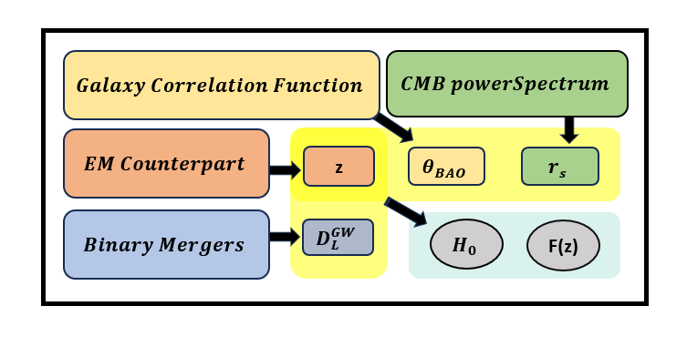
Data-driven inference of EM luminosity distance: We employ a data-driven methodology to determine the EM luminosity distance, which leverages measurements of the angular diameter distance, , obtained from the angular peak position of the BAO () observed in large scale structures across various redshifts [60]. This approach utilizes the Etherington’s distance duality relation, which establishes a fundamental connection between the EM angular diameter distance and the EM luminosity distance . The distance duality relation is given by: . This relation is derived from the fact that in a universe described by the cosmological principle (isotropy and homogeneity), the amount of light emitted from a source spreads out over an increasing area as it travels through the expanding universe. The EM angular diameter distance measures how large an object appears on the sky for a given physical size, while the EM luminosity distance relates to how bright an object appears based on its intrinsic luminosity. The factor of arises because of the cosmological redshift , which affects both the wavelength of the photons and the flux of the light received. Specifically, one factor of accounts for the redshift stretching the wavelength, thereby reducing the energy per photon, and the second factor of accounts for the time dilation effect, which reduces the rate at which photons are received. Thus, this relation allows us to convert measurements of the EMA angular diameter distance, which are typically easier to obtain from observations such as the BAO, into the EM luminosity distance needed for cosmological analyses.
The BAO peak position, as identified in the galaxy two-point correlation function, provides a direct observational basis for this calculation. The associated angular scales connect to the comoving sound horizon up to the redshift at the drag epoch () through the relationship
| (2.6) |
Substituting in Equation (2.4) with and applying the distance duality relation for EM observations, we define the function [61, 57]
| (2.7) |
Here, the comoving sound horizon at the drag epoch, , is approximated to be about 1.02 times the comoving sound horizon at the redshift of recombination (), which is . This factor is derived from CMB observations, specifically from the position of the first peak in the CMB temperature power spectrum, expressed as [62, 63, 64].
In this framework, is determined from GWs events, is extracted from galaxy two-point correlation functions, and is deduced from CMB temperature fluctuations. The redshift of GWs sources can be inferred from their EM counterparts, typically observable in events involving bright standard sirens. This methodology is illustrated by a schematic diagram in Figure 1. Consequently, the combination of these measurable quantities should conform to a consistent value across all redshifts if GR and the standard CDM cosmological model hold true. However, any deviations from these established theories could be identified through changes in these measurements across different redshifts. It is crucial to note that while is model-dependent and varies above , it remains constant at lower redshifts. Thus, any errors in the determination of would affect the absolute scale of , but not its redshift-dependent trend.
Future discussions will present results considering both independently and jointly with the Hubble constant , allowing for corrections based on potential inaccuracies in the estimated sound horizon due to erroneous Hubble constant values. This analysis supports the exploration of deviations from GR and the canonical dark energy equation of state () using a variety of observational probes. Previous studies [61] have explored parametric deviations from GR; however, our non-parametric approach using enables a detailed, redshift-specific reconstruction of deviations from GR through multi-messenger observations.
3 GW mock samples for LISA
3.1 Modelling the astrophysical population of LISA source
The formation and evolution of MBBHs and their co-evolution with host galaxies pose fundamental questions in astrophysics, with implications for understanding the regulation of star formation and the growth of galaxies [65, 66]. While active galactic nuclei (AGN), powered by growing MBBHs, are believed to play a crucial role in these processes, many aspects of MBBHs growth and AGN feedback mechanisms remain poorly understood [67, 68]. One significant challenge in studying MBBHs is related to the difficulty of observing their early evolution at high redshifts. Traditional observational methods are limited to detecting only the most luminous and rapidly growing MBBHs. GWs provide a promising avenue for probing the history of MBBHs, as their propagation through the universe is essentially unobstructed [69]. The future space-based GWs detector LISA will be particularly instrumental in this area. These binaries lie within the LISA band, and LISA’s capabilities will allow for observations deep into high redshifts, shedding light on the formation and evolution of MBBHs [70]. As a consequence, our understanding of the formation and evolution of MBBHs currently heavily relies on theoretical models. Semi-analytic models of galaxy and MBBHs formation and evolution serve as powerful tools for this[71, 72, 73, 74, 75]. These models link the hierarchical formation of dark matter halos to the evolution of galaxies and their MBBHs, capturing a wide range of galaxy formation physics [76, 77, 72, 78]. In these models, the formation of MBBHs begins with the merger of two galaxies embedded in their dark matter halos. The subsequent evolution of MBBHs proceeds through various stages, from separations of 10s-100s kpc down to a few hundred pc, and eventually to separations of 0.001–0.01 pc, where GWs emission drives the MBBHs to coalesce. The dynamical evolution of MBH binaries is influenced by interactions with their stellar and gaseous environments, as well as with other MBBHs through three/four-body interactions [79, 80]. However, fully hydrodynamic simulations, which incorporate the complex physics involved in MBBHs evolution, often suffer from poor resolution and are constrained to relatively small volumes, resulting in limited statistical power [81, 82, 83, 84, 85, 86, 87, 88]. Additionally, these simulations are computationally very demanding. While cosmological simulations have been employed to study the evolution of unresolved MBBHs, they generally necessitate significant post-processing and involve considerable simplifications. The formation and evolution of MBBHs and their co-evolution with host galaxies rely heavily on several key ingredients. These include the initial mass function of the MBH seeds, the delays between galaxy mergers and MBBHs mergers. These factors introduce complexities in modeling the dynamics and growth patterns of MBBHs. The literature presents a variety of seed models, delay models, reflecting the diverse theoretical approaches to these phenomena [71, 72, 73, 74, 75, 89, 90].
Seed Model: There are mainly two classes of seed models in the semi-analytical modeling of MBBHs formation: the Light-Seed (LS) and Heavy-Seed (HS) models. The LS model suggests that MBH seeds are remnants of Population III stars from high-redshift, low-metallicity environments, with masses centered around 300 solar masses and a standard deviation of 0.2 dex. These seeds are located in the most massive halos formed from the collapse of 3.5-sigma peaks in the matter density field at redshifts greater than 15, allowing for mildly super-Eddington accretion rates. In contrast, the HS model posits that MBH seeds form through the collapse of protogalactic disks due to bar instabilities, typically reaching masses of approximately solar masses, and are found in similar high-redshift halos but with accretion rates capped at the Eddington limit. The choice between these models affects the formation and evolution of MBBHs, impacting the observed event rates and characteristics of MBBHs mergers. This differentiation is crucial for understanding the astrophysical processes leading to MBBHs and their subsequent mergers [91, 92, 69, 93, 88]. Recent observations by the James Webb Space Telescope (JWST)[94] provide compelling evidence favoring the HS model [95]. JWST has detected extremely luminous quasars at redshifts greater than 7, suggesting the presence of very massive black holes already in the early universe[96]. The inferred masses of these early quasars are more consistent with the higher initial masses predicted by the HS model, as the rapid formation and growth required to reach such masses challenge the LS model’s predictions. These findings indicate that massive black hole seeds might have formed through more efficient, direct collapse mechanisms as proposed by the HS model[97].
Delay Models: In the study of MBBHs formation, time delays play a crucial role by affecting the evolution and eventual merger of these systems. These delays stem from various mechanisms, including dynamical friction, galaxy mergers, and the internal dynamical evolution of MBBHs within galaxies [72, 73, 98, 20]. The impact of these time delays is modeled through different scenarios, each with distinct implications for merger rates and characteristics[99, 69, 100, 101].
All of these factors and their combinations affect the event rate and the mass model of these MBBHs, which are crucial for understanding the range of scenarios detectable by LISA (for more details, see reference [69, 72]). These elements collectively influence our predictions of the frequency and characteristics of MBBHs merger events. The actual mechanisms of MBH mergers and the corresponding mass models remain largely unknown. The total number of compact binary coalescences per unit redshift is estimated by the equation
| (3.1) |
where represents the comoving volume element, and indicates the merger rate. To capture the wide range of possible merger rate scenarios, we parameterize the merger rate using a combination of two Gaussian distributions and a power law, as described by the following equation.
| (3.2) |
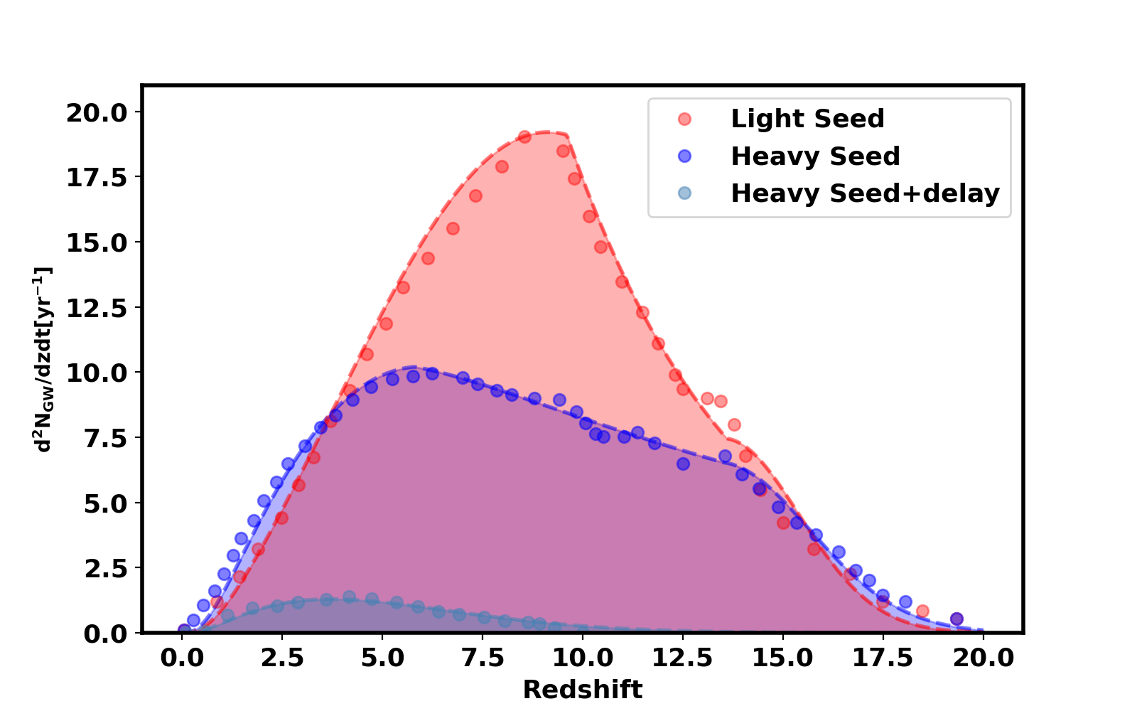
where is the overall normalization, is the mean of the left Gaussian distribution, is the standard deviation of the left Gaussian distribution, is the mean of the right Gaussian distribution, is the standard deviation of the right Gaussian distribution, and is the decay parameter of the exponential function. This approach is motivated by the need to cover all possible variations in the merger rate. Different scenarios can lead to different distributions of mergers, and a flexible parametric form allows us to represent this diversity. The Gaussian distributions help capture localized features in the merger rate, while the power law accounts for the broader trends over redshift. By configuring these components with distinct parameters, we can match a variety of theoretical models and observational constraints. Similarly, the mass model is described using variable parameters that account for different theoretical combinations of the aforementioned factors. For each unique parameter set in the merger and mass models, the predicted number of observable events varies. By integrating Equation 3.1, we calculate the total number of events, allowing us to predict the observable merger events for LISA under different theoretical scenarios. Figure 2 displays the merger rates for three distinct MBBH models using LISA. The Light Seed model involves light MBBH seeds derived from Light Seed stars, considering the temporal delays between MBBHs and galaxy mergers, thereby providing a more conservative estimate. The Heavy Seed+delay model assumes heavy MBBH seeds originating from the collapse of protogalactic disks with similar delays, while Heavy Seed omits these delays, offering an optimistic scenario for LISA event rates.
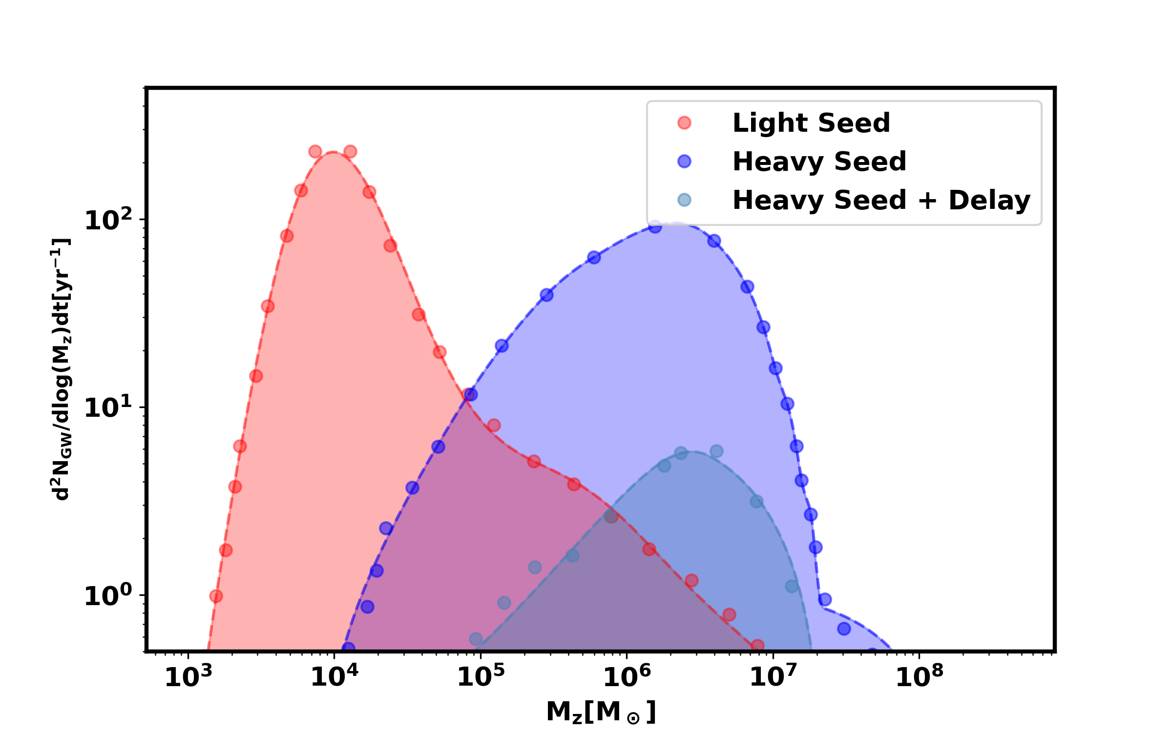
Each model is fitted using two Gaussian distributions and a power law function, as defined in Equation 3.2, and is depicted with dashed lines in Figure 2. The dotted points in Figure 2 represent data from semi-analytical simulations, as referenced in[69, 72]111https://people.sissa.it/~barausse/catalogs/readme.pdf. The solid lines are obtained by fitting these data using Equation 3.2, and all parameter values are listed in Table 1. This figure also illustrates the corresponding total redshifted mass models for these scenarios in terms of the individual masses and . In addition to the total mass, another crucial parameter for binary systems is the mass ratio (, where ). In this analysis we are interested in measuring any deviation from GR on the cosmological scale. So, we particularly focus on the high matched filtering signal to noise ratio (SNR) events in this analysis so that the uncertainty on any inferred deviation from GR is minimal. So, we consider events above SNR of fifty and only a sub-set of high SNR events are assumed to have EM counterparts. As the events with highest matched filtering SNR are those with mass ratio () equal to one, we limit our analysis only for in this analysis. Also, as it is currently unclear on how many LISA sources can have EM counterparts, we obtain forecast on the parameter for different scenarios of number of events with EM counterpart in this analysis, ranging from about to events in four years with matched filtering SNR above fifty.
However, it is important to note that LISA binaries can detectable for mass ratios less than one as well and a fraction of them can also have EM counterpart. In this analysis we consider only high SNR events and make a pessimistic choice by not considering EM counterpart to sources. For q within the range of to , the probability on defined as in the range of q values to is always at least 50% for flat ( constant) and for positive power law distributions with [102]. This percentage decreases if we assume a power law with a negative exponent in q. For other distributions, we have shown the results in Appendix B. To select a fraction of sources with the value of mass ratio close to one having EM counterpart, in this analysis we consider scenarios, namely (fiducial case) and of the total events after applying the SNR cutoff. We also consider a pessimistic case with only six events detected up to redshift with EM counterpart in four years, which corresponds to a scenario of about events for the Light Seed model and Heavy Seed model, and about events for the Heavy Seed+ delay model.
| Model | ||||||
|---|---|---|---|---|---|---|
| Light Seed | 0.056 | 9.6 | 13.6 | 4.8 | 1.9 | 0.21 |
| Heavy Seed | 0.028 | 5.8 | 13.5 | 5 | 2.3 | 0.04 |
| Heavy Seed + Delay | 0.0045 | 1.5 | 1.8 | 10.5 | 4.5 | 0.02 |
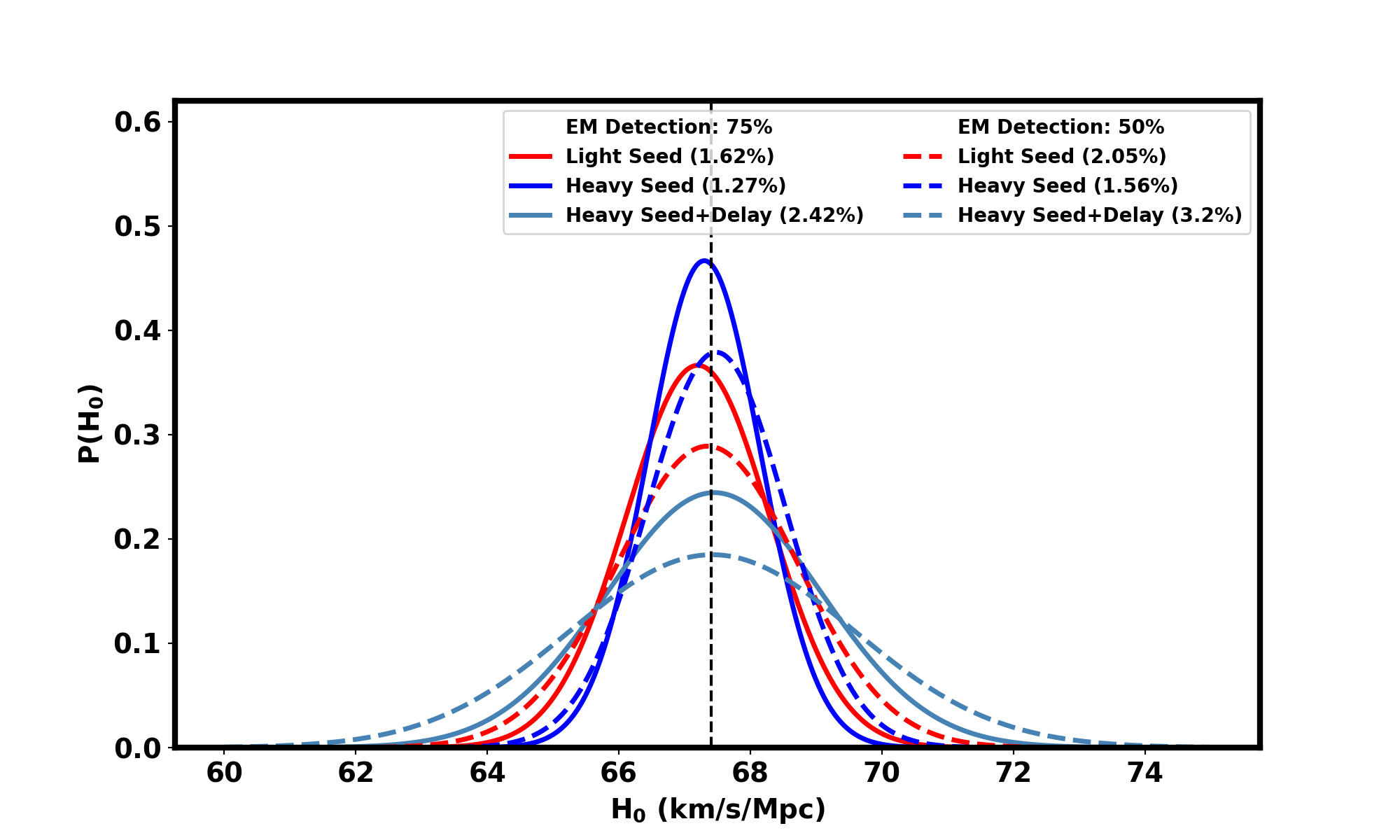
Galaxy simulations to forecast the EM counterparts for massive binary mergers typically assume a well-understood evolution of galaxies and star formation rates, calibrated from large-scale surveys. However, simulating the formation and distribution of galaxies, especially at high redshifts, comes with significant uncertainties[103, 104, 105]. One of the major challenges arises from the assumptions about gas accretion, feedback processes, and the precise merger history, which can vary significantly across different simulation models. Recent observations from the JWST have further complicated our understanding of the high-redshift universe. JWST has revealed a higher abundance of massive galaxies and earlier star formation than previously predicted, challenging existing models of galaxy formation and evolution. JWST has also detected a variety of galaxies with different dust and gas content, which directly affects the probability of producing an EM counterpart. Galaxies rich in gas are more likely to produce bright EM counterparts during binary mergers. Given these uncertainties, we assume that approximately 75% and 50% of massive binary mergers may have observable EM counterparts, depending on their redshift and environment. We have also shown the results for scenarios with and bright sirens in the appendix A. This assumption reflects the current understanding of galaxy formation processes and the likelihood that such mergers would occur in gas-rich environments, which are more conducive to generating EM radiation. While these fractions are estimates, they align with predictions from theoretical models and observational data, with the emerging JWST results suggesting a broader range of environments that could host potential EM counterparts. The models considered here are related to different theoretical approaches to MBBHs formation and evolution, significantly affecting the predicted total mass distributions and influencing the detectability of merger events by LISA. The plots effectively demonstrate how variations in initial assumptions about MBBHs seed formation and merger delays impact the mass spectrum observable by future missions. It is important to that all of these events cannot be detected due to the limitations imposed by the sensitivity of detectors. The calculation of the matched filtering SNR is essential to determine which events are detectable.
3.2 Signal to Noise Ratio (SNR) for LISA source
The matched filtering SNR, denoted as , is crucial for detecting GW events as it quantifies the GW signal’s strength relative to the background noise. An event is deemed detectable if its SNR surpasses a predefined threshold, . The optimal SNR for a GW emitted by a binary system is defined by the equation [106, 107, 108]
| (3.3) |
where represents the Fourier transform of the GWs strain, while denotes the power spectral density of the detector noise.
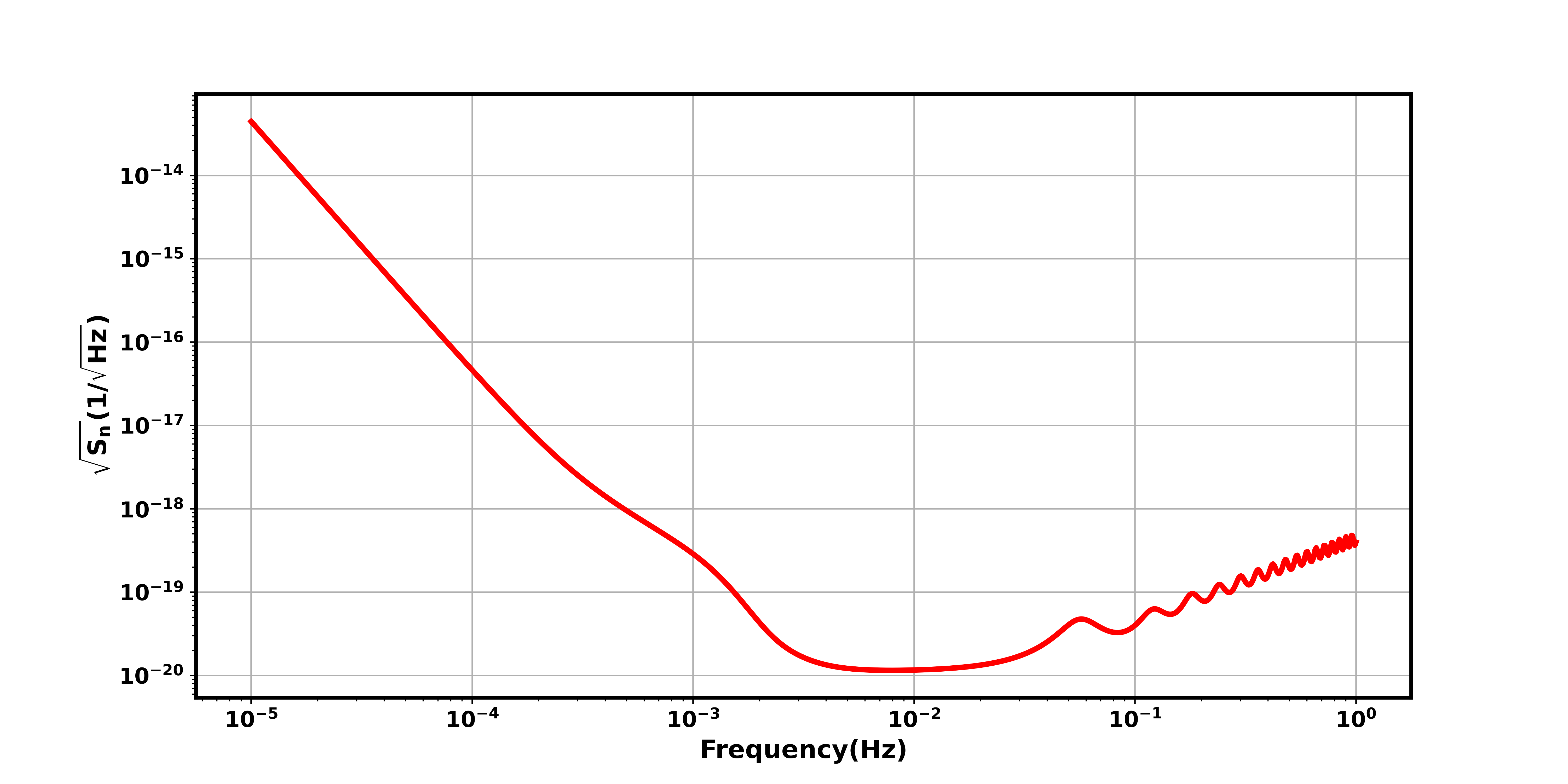
For , we adopt the semi-analytical forms from [109], as shown in Figure3, and and are the boundaries for the frequency integral. In our study, for the computation of the SNR, we set to the frequency of the innermost stable circular orbit () and to the frequency one year prior to , considering our observation period is one year. We do not include the Galactic background noise in the power spectral density. The Galactic background can have an impact on the overall noise, which in turn affects the number of detectable events.
Specifically, is expressed as
| (3.4) |
with denoting the strain amplitude
| (3.5) |
where is the chirp mass, is the mass ratio, is the luminosity distance to the source, is the speed of light, and is the phase of the waveform [110]. The factor depends on the inclination angle and the detection antenna functions and
| (3.6) |
The antenna functions are defined by[109]
| (3.7) | ||||
| (3.8) |
where and determine the source’s location in the sky, and relates to the orientation of the binary system with respect to the detector [111]. Consequently, the SNR formula becomes
| (3.9) |
where . According to [112], averaging over many binaries, the inclination angle, and sky positions, follows the distribution
| (3.10) |
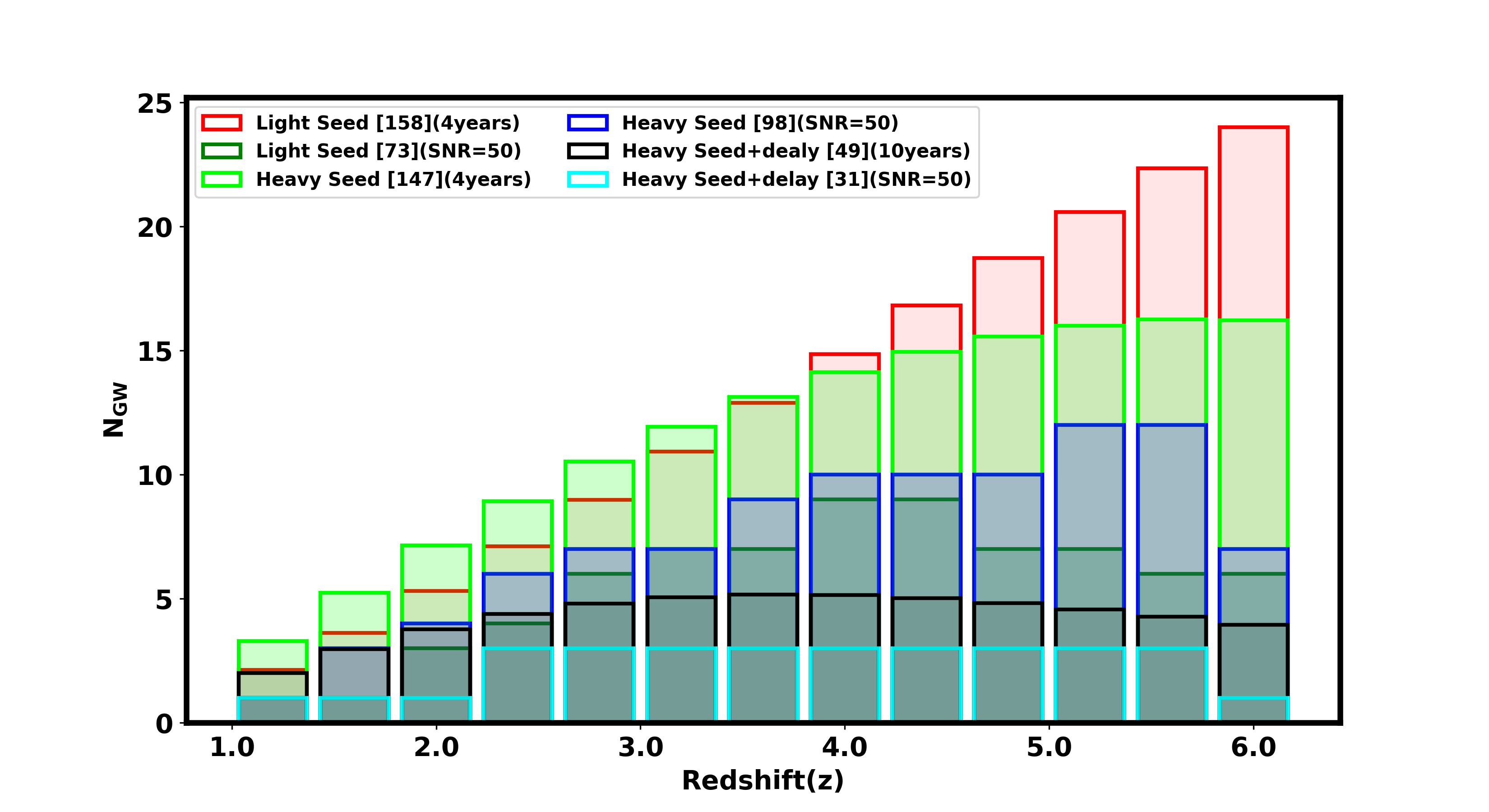
In this study, we investigate various merger and mass models, recognizing that our understanding of these models is still incomplete. By examining different scenarios, we demonstrate how different assumptions about the formation and evolution of MBBHs impact the measurements of using LISA sources. To estimate the total number of events, we integrate using Equation 3.1 and determine the number of merging events within each redshift bin, selecting a bin size of . Figure 4 displays the number of events binned by redshift for the Light Seed, Heavy Seed, and Heavy Seed + Delay models. The total number of events for each model, along with the observation years, is summarized in Table 2. For each event, we use the inverse transform method to derive the total mass of the binary system and the parameter from their probability distributions. We then generate an equal-mass binary system and calculate the SNR using Equation 3.9.
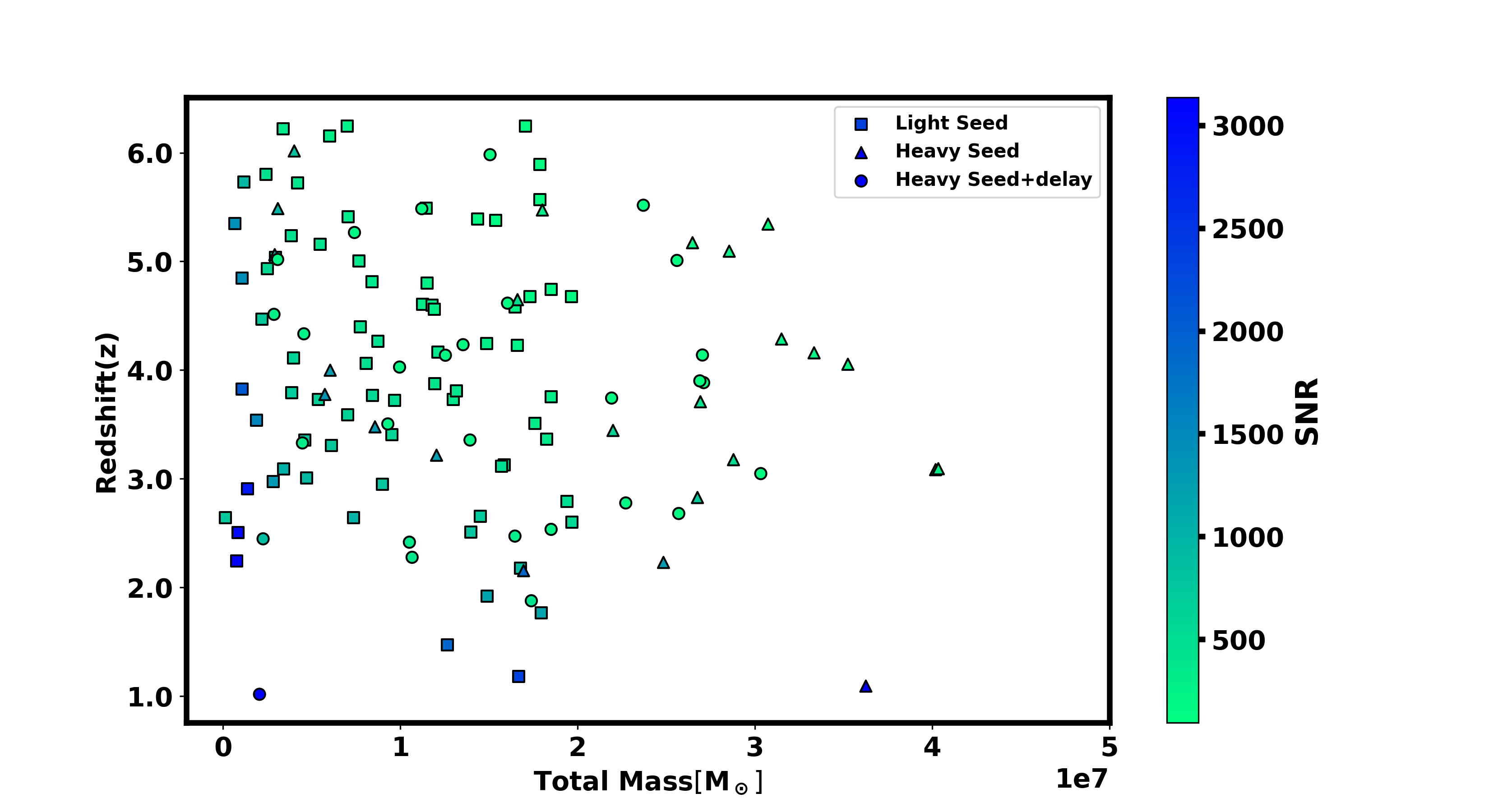
The events with an SNR exceeding the threshold are selected. Since we only consider a mass ratio of 1 when generating the binary sources, we retain of the events after the SNR cutoff. The number of events selected if only are retained is also noted and listed in Table 2. In Sec. A, we have also shown the results for different fractions of bright standard sirens detectable from LISA. For comparison, in [102], it was found that, for a mission duration of 5 years with an 80% duty cycle up to a redshift of 10 and an SNR cutoff of 10, there were a few hundred events for both light seed and heavy seed scenarios, and about 30 events for the heavy seed with delay scenario. Here, we consider a more pessimistic choice for SNR and redshift when selecting EM bright sources, as we focus only on high SNR golden events for testing GR (see Sec. 7 and appendix A). The detection probability for the Light Seed model is lower compared to the other two models because its mass distribution peaks at much lower values, resulting in reduced signal strength and, consequently, lower SNR. Figure 5 illustrates the total mass of the two components of the binary system as a function of the redshift of the selected events, with an SNR threshold of fifty.
| Model | (years) | Total Events | Selected (75%) | Selected (50%) | 1 Event Detectability |
| LS | 4 | 158 | 73 | 49 | 6.12% |
| HS | 4 | 147 | 98 | 66 | 4.54% |
| HSD | 10 | 49 | 31 | 21 | 14.28% |
3.3 LISA Source Parameter Estimation
LISA will consist of a constellation of three spacecraft forming a giant equilateral triangle in space, each containing free-falling test masses. Lasers measure the minute changes in distance between these masses, changes induced by passing gravitational waves. However, a significant challenge in detecting these waves is the overwhelming noise from laser frequency fluctuations [24]. To combat this, LISA uses Time-Delayed Interferometry (TDI), a sophisticated data processing technique that combines the laser measurements in a way that reduces noise by several orders of magnitude, making the subtle signals of gravitational waves detectable. The parameter estimation process in LISA involves several complex steps. First, the raw data from the TDI observables specifically the second-generation observables X, Y, and Z, which accommodate the fact that the spacecraft formation allows for non rigid arm lengths are transformed into the A, E, and T channels [113, 114, 115, 116, 117, 118, 119]. These channels are designed to be approximately uncorrelated in terms of their noise properties, improving the clarity and reliability of the data for further analysis.
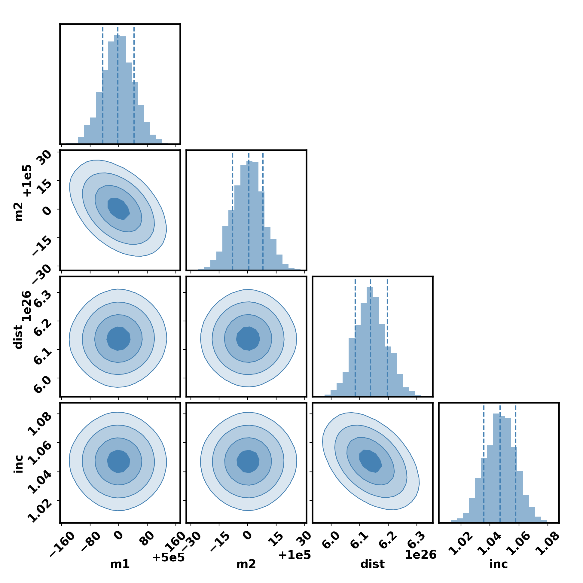
To study the GW events detected by the LISA, it is essential to estimate the parameters of these sources. The process of parameter estimation for LISA sources is quite different from that used for ground-based observatories like LIGO, Virgo, and KAGRA [120]. For our analysis of LISA sources, we employ the BBHx Python package[121] , which is specifically designed for this purpose. Our methodology involves generating waveforms using BBHx [121], which incorporates the IMRPhenomD [20, 122] waveform approximation model. We obtain the waveform for a one-year observation period of the LISA sources. Subsequently, we use BBHx [121] to calculate the likelihood of the generated waveforms. For the estimation of the posterior distributions of key parameters for this study specifically, the masses of the black holes ( and ), the luminosity distance (), and the inclination angle () we constrain the priors of all other parameters to delta functions. Finally, for the parameter estimation, we employ the Dynesty [123] sampler. Among these, the posterior of is particularly crucial for our study, as it will be used for the inference of .
The accuracy of luminosity distance measurements in GW astronomy is influenced not only by the sensitivity and configuration of the detector but also significantly by weak lensing, especially for sources detected at high redshifts by LISA [124]. Gravitational lensing affects GWs similarly to EM radiation. For GW events expected from large redshifts (), weak lensing is a common occurrence, along with the occasional strongly-lensed sources. A lens with magnification modifies the observed luminosity distance to , introducing a systematic error [125]. This lensing error, when convolved with the expected magnification distribution from a standard CDM model, significantly influences the overall measurement accuracy. In this study, we utilize the following model to estimate the error due to weak lensing [126]
| (3.11) |
The total uncertainty in the measured luminosity distance, therefore, is expressed as
| (3.12) |
where is the uncertainty derived from the detector’s setup during parameter estimation, and accounts for the lensing effects. This comprehensive approach ensures a more accurate understanding of the intrinsic properties of GW sources.
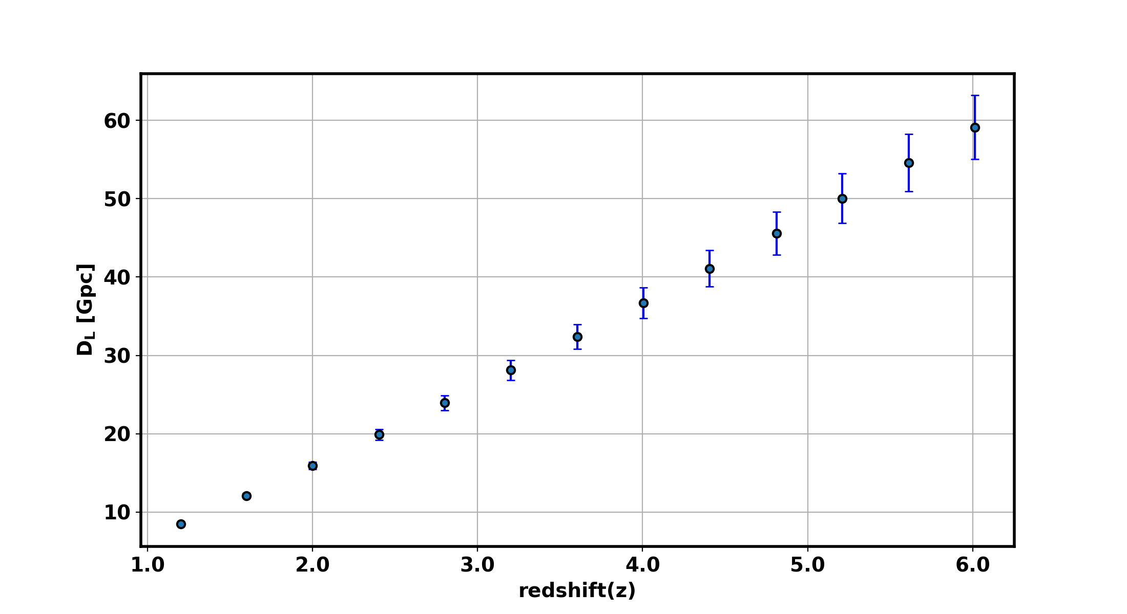
The figure 6 shows the estimated values and uncertainties for component masses, luminosity distance, and inclination angle of LISA source at a redshift of z=2.4. This highlights the potential of LISA to offer precise insights into the cosmological properties of binary systems from the early universe. The figure 7 presents the luminosity distance errors as a function of redshift for LISA sources, showcasing the variability and precision of measurements across different redshifts. Each point in the plot represents the measured luminosity distance at various redshifts, with total uncertainty, derived from two specific sources of errors: GW source parameter estimation error and WL error. This figure underscores the advanced capabilities of LISA in probing the universe’s most distant reaches, illustrating the impact of different sources of uncertainty on measurement accuracy, and paving the way for profound cosmological discoveries.
4 Identification of EM Counterparts for LISA Sources
The EM counterpart detection for LISA sources involves a sophisticated interplay of various observational techniques and instruments across multiple wavelengths. One of the primary targets for such detections is the optical emission from AGN, which can be observed using the Vera Rubin Observatory [127, 128, 129, 130]. The Vera Rubin Observatory, with its powerful 8.4-meter mirror, is capable of capturing images in the u, g, r, i, z, and y bands [131]. There are two main strategies for utilizing the Rubin Observatory in the search for LISA counterparts. The first involves sifting through archival data from the Vera Rubin Observatoryto identify potential modulations caused by the proper motion of binaries prior to their merger. The second strategy is to employ Target of Opportunity (ToO) observations, which can be triggered when a LISA event is detected, allowing astronomers to quickly point the telescope and capture fresh data. The depth of the Vera Rubin Observatorysurvey, expected to reach an apparent magnitude of around 27.5 after ten years of operations, sets the detection threshold for these observations [130, 132, 133].
To effectively detect EM radiation from merging MBBHs, it is essential to use radio and optical telescopes to target GWs sources preemptively. For selecting potential candidates that may emit EM counterparts during the inspiral phase of MBBHs, a conservative approach involves choosing GWs events with a SNR of 8 or higher and a sky localization accuracy within 10 square degrees, matching the field of view of the Vera Rubin Observatory[134, 102, 135, 25]. For this analysis we have chosen only events with SNR greater than 50, as a result the sky localization error will be better and EM counterparts can be easier to identify.
Among LISA-detected events meeting these criteria, we assume that EM emissions at merger consist of optical flares driven by accretion and radio flares and jets, as indicated by general-relativistic simulations of MBH mergers in external magnetic fields. The semi-analytical simulations within MBBHs catalogs provide detailed data on mass in stars, nuclear gas, and other parameters, which are essential for estimating the magnitude of each merger’s EM emission in both optical and radio bands [27, 136, 137, 138]. The future detection capabilities of EM facilities like Vera Rubin Observatory [139], the Square Kilometre Array (SKA) [140], and the Extremely Large Telescope (ELT)222https://www.eso.org/sci/facilities/eelt/ can be assessed by determining the expected number of detectable counterparts. While the sky localization region may contain multiple EM transients, the true EM counterpart is assumed to be efficiently identified using methods such as timing, spectrum analysis, and host galaxy information, similar to prior studies. This precise identification allows for the host galaxy to be pinpointed and the GWs parameters to be refined by fixing the sky localization angles, thereby enhancing the accuracy of the measurements.
In addition to optical observations, radio emissions, particularly those emanating from jets, provide another promising avenue for detecting EM counterparts of LISA sources. The SKA, expected to be the world’s largest radio telescope, will play a pivotal role in this effort. Significant radio emissions can be produced by the interaction between the plasma surrounding a merging binary and the magnetic fields. These emissions can manifest as flares due to the twisting of magnetic field lines or as jets driven by mechanisms like the Blandford-Znajeck effect [30]. The SKA can be employed in ToO observations to capture these radio emissions. Depending on the beaming and the orientation of the jets, the radio luminosity can vary significantly. The ability of SKA to detect these emissions is contingent upon the observed flux surpassing the instrument’s sensitivity threshold, which is set at 1 micro-Jansky for a typical frequency of 1.7 GHz [31, 141, 142, 29, 143].
In the near-infrared spectrum, the ELT is anticipated to be a vital tool for redshift measurements of host galaxies. ELT’s MICADO spectrograph will enable the precise measurement of redshifts in the IYJHK bands. The detection threshold for ELT’s spectroscopy is set at an apparent magnitude of 27.2, while for imaging, it extends to 31.3. For galaxies brighter than 27.2, the redshift measurement error is expected to be extremely small, allowing for highly accurate determinations. For fainter galaxies, between magnitudes 27.2 and 31.3, the precision of redshift measurements varies depending on the actual redshift of the source. High-redshift sources, those beyond a redshift of , can be identified by the Lyman-alpha break with a redshift error of around 0.2. For sources with redshifts between 0.5 and 5, the Balmer break can be used for redshift identification; however, the absence of observations in the optical and UV parts of the spectrum increases the redshift error to about 0.5 [144, 145, 146, 94]. Collectively, these strategies and instruments provide a comprehensive framework for the detection and study of the EM counterparts of LISA sources. By combining data across optical, radio, X-ray, and near-infrared wavelengths, a multi-faceted understanding of the processes and environments surrounding merging MBBHs and other GW sources can be gained. This multi-wavelength approach is crucial for the advancement of our knowledge of the Universe and for maximizing the revolutionary capabilities of the LISA mission.
5 Baryon Acoustic Oscillation Scale from galaxy power spectrum
BAO are patterns resembling wrinkles in the distribution density of galaxies across the universe, originating from acoustic density waves in the early universe’s primordial plasma[60, 147]. These waves were propelled by the interplay between radiation pressure and gravitational forces. As the universe expanded and cooled, leading to the decoupling of photons from baryons, a characteristic scale the sound horizon at the drag epoch () denoted by left a discernible imprint on the galaxy distribution[148, 149, 150, 151, 152].
5.1 Inference of BAO from galaxy two-point angular correlation function
The imprint manifests as a distinct peak within the two-point angular correlation function (2PACF) of galaxies, , which offers a method to measure the universe’s expansion rate across its history. To detect the BAO feature within , it is modeled using a combination of a power-law and a Gaussian component, represented by the following equation[153, 154, 155]
| (5.1) |
where are parameters representing the fit, is the width of the BAO peak, and indicates the angular position of the BAO feature. This method offers a robust standard ruler that enables independent estimates of the angular diameter distance, , further elucidating the dynamics of the universe’s expansion[156, 157, 158, 159, 160].
5.2 Modeling the two-point angular correlation function
The theoretical representation of the 2PACF, , is formulated as
| (5.2) |
where denotes the Legendre polynomial of the order, and represents the angular power spectrum. The latter is derived from the three-dimensional matter power spectrum through the integral[60, 147]
| (5.3) |
where is defined as:
| (5.4) |
incorporating , the galaxy selection function, and , the spherical Bessel function of the order, with being the comoving distance. An exponential damping factor is included to enhance the integration’s convergence in calculating the angular power spectrum, where is consistently used across all calculations, proven to have negligible effects on the scales under consideration[161]. For deriving the matter power spectrum, we employ the CAMB[162] module, configuring the galaxy selection function as a normalized Gaussian distribution. We set the standard deviation of this distribution to of its mean value, aligning it with the anticipated photo-z error from the Vera Rubin Observatory [139, 163, 164] .
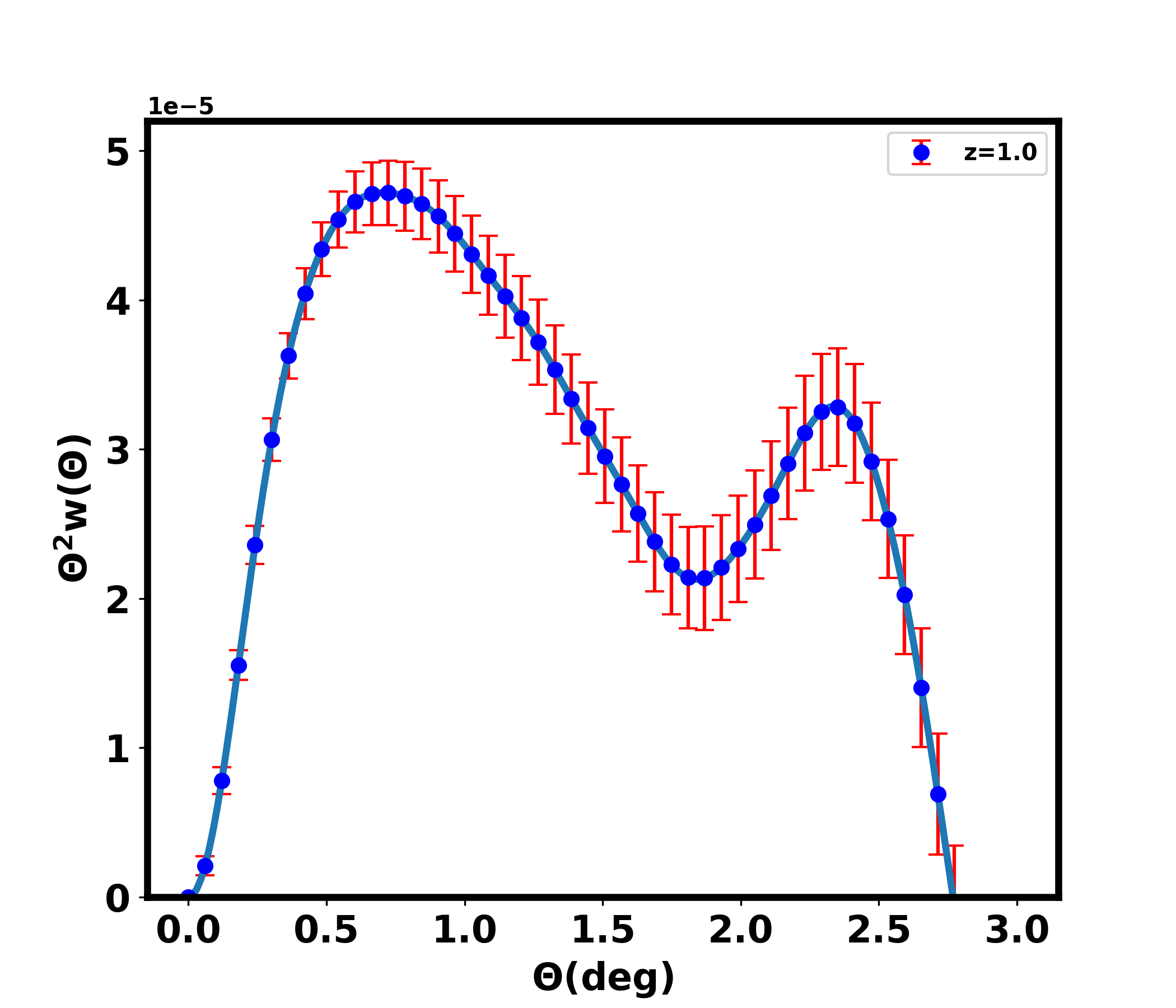
Figure 8 showcases the variation of with angular separation at a fixed redshift . A marked peak at approximately reveals the BAO scale, central to our analysis. Furthermore, the covariance of , expressed as , is computed as:
| (5.5) |
where signifies the shot noise linked to the galaxy’s number density per steradian, and is the fraction of the sky surveyed[165, 166]. A depiction (Figure 9) outlines how the covariance matrix evolves with angular separations at a given redshift(z=1), indicating a growing correlation as and increase. We have included the complete covariance matrix in the analysis, as there are sufficient correlations between different scales.
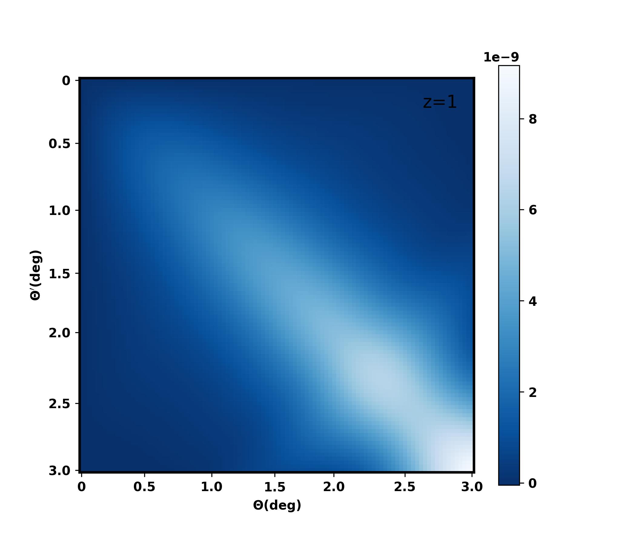
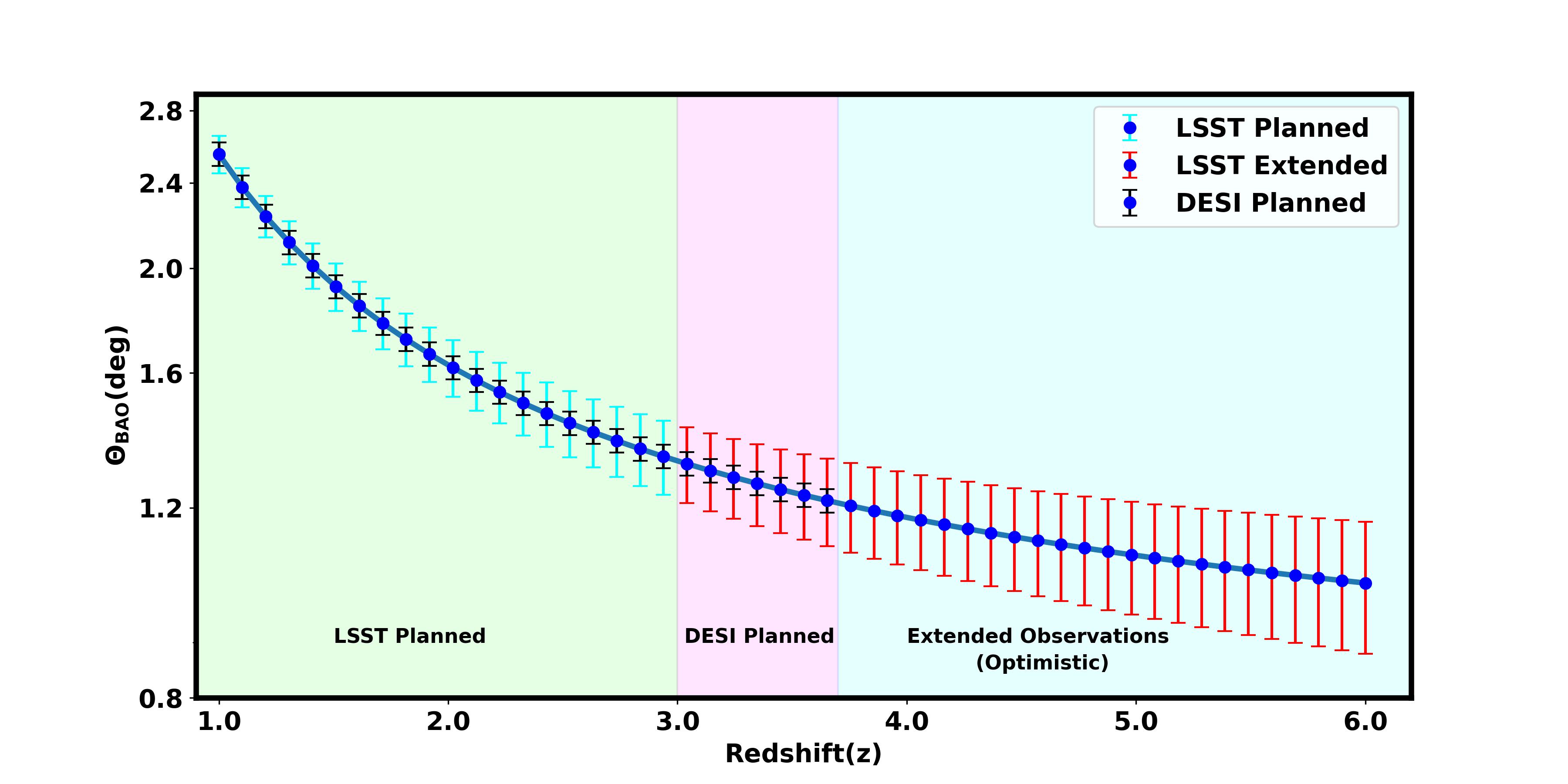
Figure 10 elaborates on the BAO scale’s variation and associated error across different redshifts, emphasizing the influence of photo-z errors. For LSST’s planned photo-z error, we illustrate the error on BAO measurements from to in cyan, showing how the expected errors will affect the precision of BAO measurements. Vera Rubin Observatory[139, 163], along with projects like Euclid [167], will significantly enhance our understanding of BAO by surveying a total area of 18,000 square degrees, extending precise measurements to higher redshifts. The figure also depicts the BAO measurement error anticipated from Dark Energy Spectroscopic Instrument(DESI) [168] up to redshift 3.7, shown in black, demonstrating the expected performance of DESI in this redshift range. The DESI is a notable five-year terrestrial survey focusing on exploring BAO and the evolution of cosmic structures through redshift-space distortions. Covering 14,000 square degrees of the sky, corresponding to a sky fraction () of 0.3, DESI aims for an accuracy better than 0.5% within the redshift intervals . Despite the lack of currently planned instruments to measure BAO beyond redshift 3.7, we extend the BAO measurements up to redshift 6 using the same photo-z error anticipated for LSST, shown in red. This extended range provides a hypothetical look at the potential capabilities of future surveys and their ability to probe deeper into the universe. This visualization provides essential insights into the variability of the BAO scale and its error with increasing redshift, highlighting a rise in relative error as the standard deviation of the selection function increases with redshift. With the capability of LISA in probing the high redshift Universe, this plot shows that future galaxy surveys with capabilities of measuring BAO beyond can bring interesting tests of fundamental physics explored in this analysis.
6 Forecast for reconstructing F(z) with redshift
6.1 Case with the fixed Hubble constant
The correlation between the EM luminosity distance at a specific redshift (z) and critical cosmological parameters, such as the BAO scale () and the sound horizon (), is succinctly expressed by the Equation 2.7. This equation is central to the analysis of the frictional term, linking it to three significant cosmological lengths: (i)GW Luminosity Distance: The distance for detectable GW events is estimated through the parameter estimation of GW events as described in Subsection 3.3. (ii)BAO Scale (): Derived from the 2PACF and expressed in Equation 5.1, this scale is utilized in a versatile manner, allowing for application across various surveys. (iii)Sound Horizon Distance: Estimated by analyzing CMB acoustic oscillations through missions like WMAP [63], Planck [64], ACTPol [169], SPT-3G [170], and CMB-S4 [171]. The first peak in the angular power spectrum at recombination reflects the sound horizon scale, measured precisely by Planck as Mpc at the drag epoch and redshift: Inferred from the EM counterparts.
To estimate the posterior distribution of as a function of redshift for GW sources, we employ a Hierarchical Bayesian framework. The posterior distribution is represented as follows [57]
| (6.1) |
In this framework, denotes the posterior probability density of . The term corresponds to the likelihood function, which represents the posterior distribution of the GW luminosity distance. In this expression, and representing the prior probabilities for the sound horizon and BAO scale, respectively. indicates the prior distribution for , reflecting pre-existing knowledge or assumptions about the frictional term before the data is considered. A flat prior from 0.1 to 2 is adopted for . This investigation focuses solely on bright sirens, assuming that the redshift of the host galaxies of the GW sources is measured spectroscopically. This assumption implies precise measurements of redshift for these sources, as the error in redshift measurements is very small compared to the errors associated with the BAO scale and distance measurements.
6.2 Case with varying the Hubble constant
In previous discussions, we concentrated on analyzing the frictional term, denoted as in Equation 2.7, under the assumption of a constant Hubble constant (). Moving forward, we expand our analysis to concurrently estimate both and . Our primary objective remains the precise determination of , while concurrently assessing . This dual estimation strategy is especially pertinent with the advent of future detectors, which will enhance our capability to probe deeper into redshifts, thus enabling either combined or independent measurements of these parameters. This methodology is particularly promising for addressing the so-called Hubble tension (for a comprehensive review [172]), the notable discrepancy between the locally measured values of and those inferred from CMB observations [173].
By employing a hierarchical Bayesian framework, we efficiently estimate these parameters using a comprehensive array of observational data, encompassing GW detections, CMB data, and large-scale structure surveys, as elaborated in earlier sections. The hierarchical integration of these datasets is meticulously designed to manage their distinct uncertainties and biases effectively. This integration produces correlated constraints that significantly enhance our understanding of cosmological dynamics, help resolve discrepancies among observational datasets, and uncover critical relationships between key cosmological parameters. The joint posterior distribution for and , based on these considerations, is formulated as follows
| (6.2) |
In this model, denotes the joint posterior probability density function for and . The likelihood function is represented by . The terms and define the prior distributions for and , respectively, encapsulating pre-existing beliefs or assumptions prior to analyzing the data. Within our hierarchical Bayesian framework, we utilize flat priors for both parameters, indicating minimal initial bias. The range for is set from 0.1 to 2.0, and for , from 40 km/s/Mpc to 100 km/s/Mpc.
7 Results
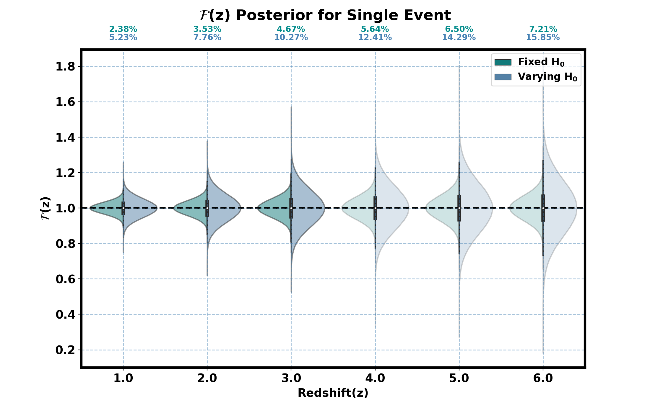
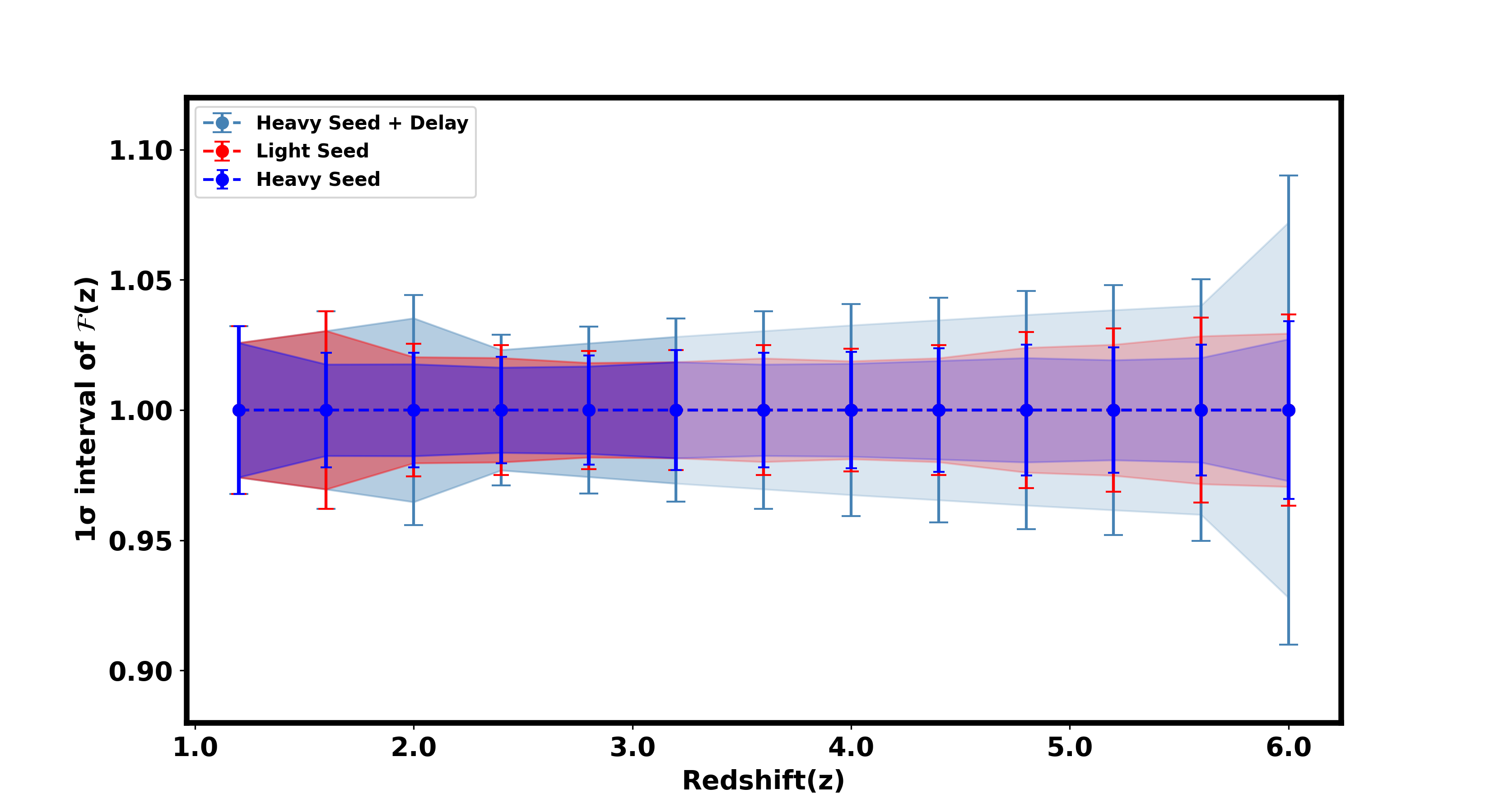
This study exclusively examines bright sirens detectable by the space-based GWs observatory LISA, focusing on events with a redshift up to across multiple population models. We present the frictional term, , measurements under two scenarios: with a fixed Hubble constant () and with a varying . The comparative results are illustrated in Figure 11 and Figure 12. Specifically, Figure 11 showcases the impact of single-event measurements, and Figure 12 highlights how event detection rates and population assumptions influence the precision of measurements.
7.1 Reconstruction of F(z)
In cases where is held constant, it acts as an overall normalization factor for across different redshifts. This setup provides a unique opportunity to normalize measurements to 1 if an independent and precise measurement of in our local universe is possible. Such normalization, particularly effective at low redshifts, helps eliminate the dependence on and demonstrates the potential deviations from GR due to the cumulative effects of modified gravity wave propagation over cosmological distances. The uncertainty in the measurement of the frictional term, , is inversely proportional to the square root of the number of GW sources, denoted as . This relationship suggests that increasing the count of GW sources detected by LISA enhances the precision of measurements. However, the accuracy improvement reaches a plateau beyond a certain number of sources, primarily due to errors associated with the BAO scale. The precision in estimating the BAO scale emerges as a critical factor limiting the refinement of estimation accuracy. Thus, advancing the accuracy of BAO scale measurements is essential for further enhancements in determining the frictional term with redshift. Essentially, optimizing the number of GW observations, alongside improvements in BAO scale accuracy and GWs luminosity distance measurements, is crucial for advancing our understanding of and probing new aspects of fundamental physics.
On the GWs front, the accuracy of relies predominantly on the precision of the luminosity distance to GWs sources, . Enhancements in measuring would significantly boost the fidelity of estimations. Given the degeneracy of with other GWs parameters, notably the inclination angle (), acquiring more accurate measurements of the inclination angle, potentially through EM counterparts, could substantially reduce uncertainties in and, by extension, refine estimates [174]. The effect of peculiar velocities on redshift inference from EM counterparts is notably critical at lower redshifts () but becomes negligible at higher redshifts [175]. Given that the majority of GW sources detected by LISA are expected to be at higher redshifts, this effect is disregarded in our analysis.
7.2 Reconstruction of F(z) and Hubble Constant
Building upon the hierarchical Bayesian framework introduced earlier to estimate with a fixed , we now extend this approach to concurrently measure and the Hubble constant, . In this extended framework, we derive the EM luminosity distance by integrating various cosmological scales, including the BAO scale, sound horizon distance, and redshift. Figures 11 provide a detailed analysis of measurements under scenarios of both fixed and varying with only six events up to . The uncertainty on the parameter increased by approximately a factor of 2 to 2.5 when is allowed to vary relative to scenarios with a fixed . This scenario with only six events corresponds to a pessimistic case with only EM bright events for the Light Seed model and the Heavy Seed model and about for the Heavy Seed+Delay model in four years of observation period. This corresponds to a single events at every redshift up to . We have shown the constraints for a few scenarios of detectable bright sirens from LISA in appendix A. If the efficiency of LISA bright sirens are less than this, then one needs to consider a longer observation period of the LISA mission for at least one detection of bright standard siren.
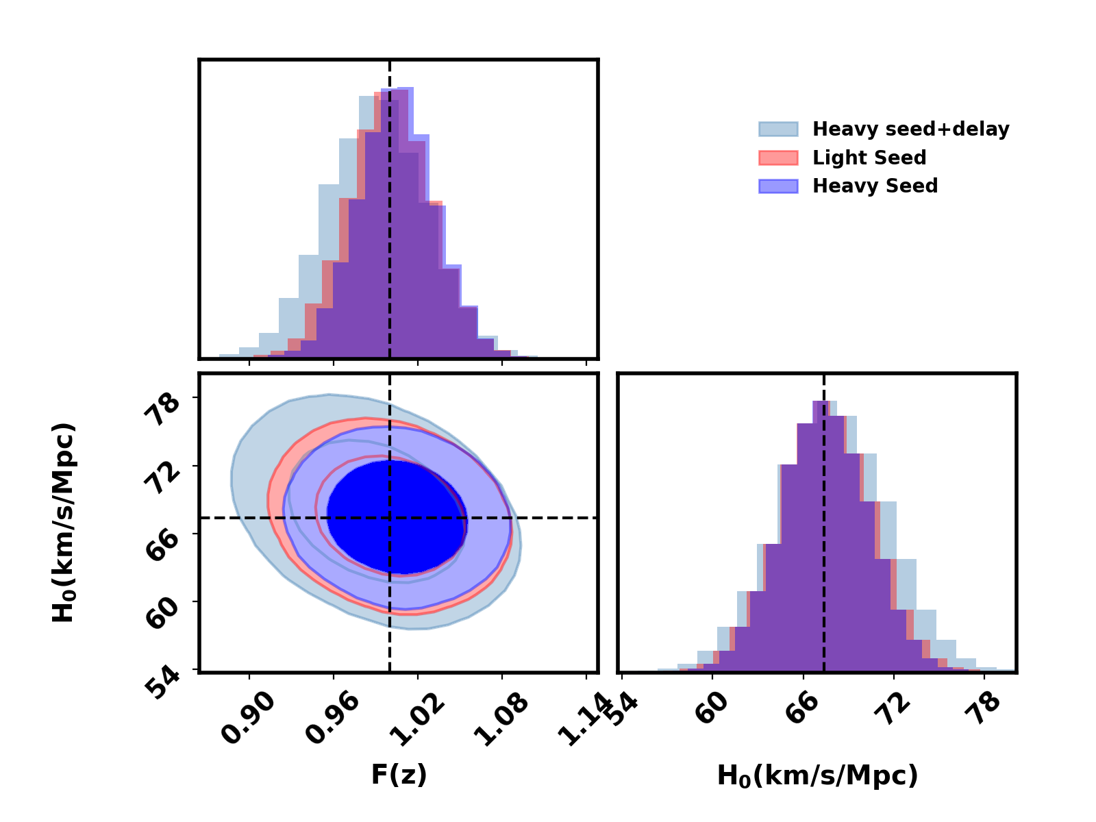
In Figure 12, we specifically illustrate the improved precision in tracking the redshift-dependent variations of the Planck mass () for MBBHs systems, emphasizing enhanced measurements in the redshift range from to . Additionally, Figure 13 illustrates the optimal joint measurements of and the Hubble constant (). In Figure 14, we show the measurement of marginalized over for the three different population models, for all events up to a redshift of . The results on and for scenario with MBBHs distribution having a mass ratio beyond is shown in the appendix B.
8 Conclusion & Discussion
In this study, we introduce a model-independent approach for investigating the frictional term in theories of gravity, capable of identifying deviations from GR in the cosmological scales across any redshift. This analysis is facilitated by bright sirens that will be observable by the upcoming space-based GWs detector LISA, which is designed to operate in the milliHertz frequency range. Building on our previous work [57, 176], we have already demonstrated a model-independent reconstruction of the frictional term using current and forthcoming ground-based GW detectors, which primarily operate in the hertz to kilohertz frequency spectrum.
We propose a novel strategy that integrates three pivotal cosmological measures as functions of redshift: the luminosity distance from GW sources , the angular scale of the BAO from galaxy surveys , and the sound horizon from CMB observations. This amalgamation provides a unique framework to scrutinize alternate theories of gravity, particularly focusing on the frictional term. Through an integrated analysis combining BAO measurements, sound horizon distances, redshiftd from EM counterpart, and GW luminosity distances, we enable a robust measurement of cosmological parameters. This approach notably improves our ability to simultaneously determine the Hubble constant () and the frictional term as a function of redshift in a model-independent way. We have demonstrated the feasibility of achieving precise measurements of the frictional term with an accuracy ranging from to up to a redshift of 6, utilizing just a single GW source detected by LISA. Additionally, we achieve a measurement of the Hubble constant with a precision of , marginalized over the measurements of deviations in the frictional term, for 4 years of observation time. This assumes that EM are detected for of the events. The accuracy of these measurements scales inversely with the square root of the number of events, which is proportional to the square root of the observation time, expressed as . Furthermore, our methodology allows for the reconstruction of the frictional term as a function of redshift without relying on any specific parametric forms, highlighting the strength and flexibility of this model-independent approach in advancing our understanding of cosmic expansion and the underlying forces.
The current BAO measurements from the Vera Rubin Observatory, Euclid, and DESI, which cover redshifts up to z=3.7. This limitation on the BAO measurements impacts our results on the reconstruction of the frictional term as a function of cosmic redshift. This limitation is illustrated in Figures 11 and 12, where we show the results using deeper colors for redshifts up to . Beyond redshift , the results are shown in fainter colors to highlight the limitations of our current planned BAO measurements, as we have used LSST-like measurements for our analysis. Improved surveys with deeper reach could potentially overcome these limitations, providing more accurate reconstructions and deeper insights into the frictional term across a wider range of redshifts.
Additionally, our proposed methodology can be adapted to incorporate dark sirens, where accurately determining the redshift is critical. For this, the three-dimensional clustering of GW sources with galaxies is employed to deduce redshifts, as highlighted in prior studies. [177, 178, 179, 180, 181, 176]. It is important to note that the current analysis focuses strictly on bright sirens. This focus necessitates the exclusion of certain GW sources such as EMRIs and stellar mass BHBs, which typically do not have EM counterparts. Furthermore, our study limits its scope to redshifts up to due to the increasing difficulty in detecting EM counterparts beyond this point. Incorporating dark sirens, which do not have EM counterparts, could significantly refine the accuracy of our frictional term measurements. The extension of our approach to include dark sirens could lead to more precise determinations of the frictional term, thereby enhancing our understanding of the fundamental principles of gravity.
Acknowledgements
This work is part of the ⟨data|theory⟩ Universe-Lab, supported by TIFR and the Department of Atomic Energy, Government of India. We would like to thank Enrico Barausse for providing comments on the draft. We also express gratitude to the computer cluster of ⟨data|theory⟩ Universe-Lab and the TIFR computer center HPC facility for computing resources. We acknowledge the use of the following packages in this work: Astropy [182, 183], Bilby [184], Pandas [185], NumPy [186], Seaborn [187], CAMB [162], Scipy [188], Dynesty [123], emcee [189], Matplotlib [190] and BBHx [121].
Appendix A Impact of Electromagnetic Counterpart Detection on and Measurements
In this section, we present a few cases of bright sirens detectable from LISA and summarize the best measurements of and the combined error on for three different models: Light Seed, Heavy Seed, and Heavy Seed + Delay. Each table provides results for various event selections, including 75%, 50%, 25%, and 10% of selected events. The tables detail the maximum redshift up to which a source is detected in LISA (), the total number of GW events () up to , and the associated precision on and . For we quote the minimum uncertainty and corresponding redshift, and for the Hubble constant, we mention the uncertainty after combining events.
Tables 3, 4, and 5 present the results for the Light Seed model, Heavy Seed model and the Heavy Seed + Delay model respectively. For each model, the tables highlight the least percentage error in at specific redshifts, and the overall combined error on . Note that for the 10% selection case, where no events are available, it is denoted as "–". These tables illustrate how the precision of and varies with the number of selected events and their redshift range, reflecting the impact of different selection thresholds on measurement accuracy.
| Bright events | Least uncertainty on | Combined uncertainty on | ||
| 75% Selected | 6 | 73 | 2.65% at z=1.2 | 1.62% |
| 50% Selected | 6 | 49 | 2.65% at z=1.2 | 2.05% |
| 25% Selected | 6 | 23 | 3.57% at z=2.0 | 3.40% |
| 10% Selected | 5.2 | 6 | 5.02% at z=3.2 | 6.42% |
| Bright events | Least uncertainty on | Combined uncertainty on | ||
|---|---|---|---|---|
| 75% Selected | 6 | 98 | 2.62% at z=1.2 | 1.27% |
| 50% Selected | 6 | 66 | 2.62% at z=1.2 | 1.56% |
| 25% Selected | 6 | 32 | 3.02% at z=1.6 | 2.60% |
| 10% Selected | 6 | 9 | 4.51% at z=2.8 | 4.50% |
| Bright events | Least uncertainty on | Combined uncertainty on | ||
|---|---|---|---|---|
| 75% Selected | 6 | 31 | 2.63% at z=1.2 | 2.42% |
| 50% Selected | 6 | 21 | 2.63% at z=1.2 | 3.20% |
| 25% Selected | 5.6 | 9 | 4.26% at z=2.4 | 6.82% |
| 10% Selected | – | – | – | – |
Appendix B Measurements for Different Mass Ratio Distributions
In this section, we extend our analysis of and using LISA bright sirens by considering different mass ratio distributions for binary mergers. Previously, we presented results assuming mass ratio . Here, we explore the impact of varying mass ratios on the measurements of and . Specifically, we investigate mass ratio distributions following , where is defined as the ratio of the component masses and ranges from to 1. We consider two selection criteria for these distributions: 75% and 50%, corresponding to the different proportions of systems retained based on their mass ratios. This approach allows us to understand how variations in the mass ratio distribution affect the detectability and measurement precision of bright sirens.
In Table 6 we provides a summary of the total number of events and the number of detected events for different merger models with an SNR threshold of 50, categorized by the mass ratio selection criteria of 75% and 50%. The results show that the distribution of mass ratios does not significantly affect the number of detected events, as our study is limited to sufficiently low redshifts where most events are very bright. Comparing these findings with the results in Table 2, we find that the number of detected events differs by approximately 2-7%, depending on the model. This variation is most pronounced in the high-redshift portion of our analysis.
| Model | (years) | Total Events | Selected (75%) | Selected (50%) | 1 Event Detectability |
| LS | 4 | 158 | 68 | 44 | 6.82% |
| HS | 4 | 147 | 96 | 64 | 4.69% |
| HSD | 10 | 49 | 29 | 20 | 15.01% |
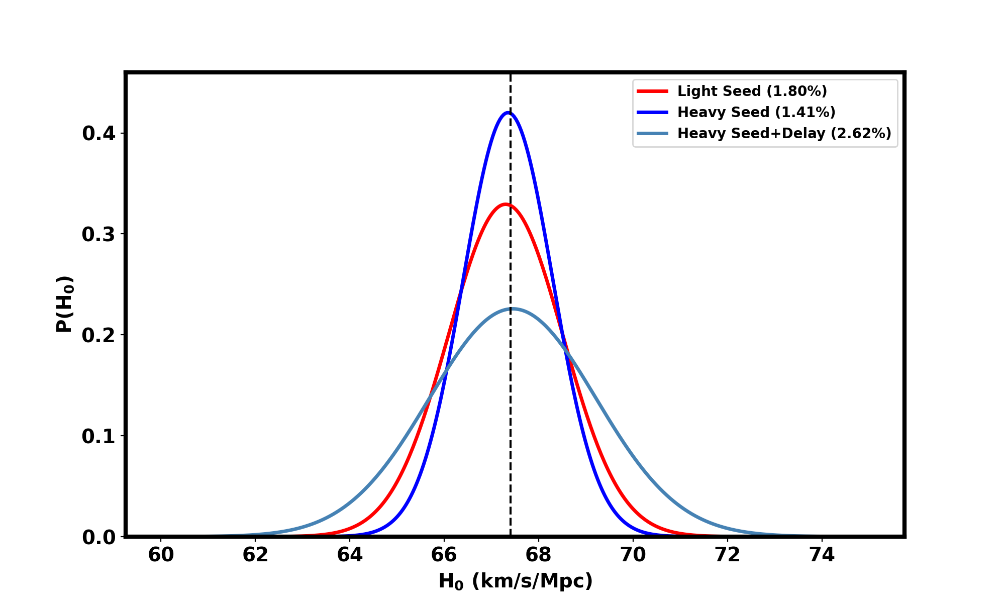
Figures 15 and 16 illustrate the results on the feasibility of inferring the parameter using the mass ratio distribution with LISA. Figure 15 presents the precision in reconstructing the redshift evolution of the Planck mass, , highlighting LISA’s measurement capabilities up to a redshift of 6, with reduced accuracy beyond a redshift of 3.0 due to limitations in BAO scale measurements. Figure 16 shows the posterior distribution of the Hubble constant () for events up to a redshift of , assuming that EM counterparts are detected for 75% of the events.
Here, we have used a power-law distribution proportional to with . The measurements of and will improve for any , as the area under the curve of these distributions increases when approaches 1. This means that the probability of obtaining nearly equal mass binaries is higher, leading to a higher SNR and, consequently, more events. Conversely, for , the measurements become less accurate because the area under the curve decreases, reducing the likelihood of nearly equal mass binaries, resulting in a lower SNR and fewer events.

References
- [1] K. S. Thorne, Gravitational waves, arXiv preprint gr-qc/9506086 (1995) .
- [2] B. S. Sathyaprakash and B. F. Schutz, Physics, astrophysics and cosmology with gravitational waves, Living reviews in relativity 12 (2009) 1.
- [3] B. P. Abbott, R. Abbott, T. Abbott, M. Abernathy, F. Acernese, K. Ackley et al., Observation of gravitational waves from a binary black hole merger, Physical review letters 116 (2016) 061102.
- [4] B. P. Abbott, R. Abbott, T. Abbott, M. Abernathy, F. Acernese, K. Ackley et al., Gw151226: observation of gravitational waves from a 22-solar-mass binary black hole coalescence, Physical review letters 116 (2016) 241103.
- [5] L. Scientific, B. P. Abbott, R. Abbott, T. Abbott, F. Acernese, K. Ackley et al., Gw170104: observation of a 50-solar-mass binary black hole coalescence at redshift 0.2, Physical review letters 118 (2017) 221101.
- [6] B. P. Abbott, R. Abbott, T. Abbott, F. Acernese, K. Ackley, C. Adams et al., Gw170817: observation of gravitational waves from a binary neutron star inspiral, Physical review letters 119 (2017) 161101.
- [7] A. Goldstein, P. Veres, E. Burns, M. Briggs, R. Hamburg, D. Kocevski et al., An ordinary short gamma-ray burst with extraordinary implications: Fermi-gbm detection of grb 170817a, The Astrophysical Journal Letters 848 (2017) L14.
- [8] J. Aasi, B. Abbott, R. Abbott, T. Abbott, M. Abernathy, K. Ackley et al., Advanced ligo, Classical and quantum gravity 32 (2015) 074001.
- [9] F. a. Acernese, M. Agathos, K. Agatsuma, D. Aisa, N. Allemandou, A. Allocca et al., Advanced virgo: a second-generation interferometric gravitational wave detector, Classical and Quantum Gravity 32 (2014) 024001.
- [10] T. Akutsu, M. Ando, K. Arai, Y. Arai, S. Araki, A. Araya et al., Overview of kagra: Detector design and construction history, Progress of Theoretical and Experimental Physics 2021 (2021) 05A101.
- [11] M. Saleem, J. Rana, V. Gayathri, A. Vijaykumar, S. Goyal, S. Sachdev et al., The science case for ligo-india, Classical and Quantum Gravity 39 (2021) 025004.
- [12] D. Reitze, R. X. Adhikari, S. Ballmer, B. Barish, L. Barsotti, G. Billingsley et al., Cosmic explorer: the us contribution to gravitational-wave astronomy beyond ligo, arXiv preprint arXiv:1907.04833 (2019) .
- [13] M. Punturo, M. Abernathy, F. Acernese, B. Allen, N. Andersson, K. Arun et al., The einstein telescope: a third-generation gravitational wave observatory, Classical and Quantum Gravity 27 (2010) 194002.
- [14] KAGRA, VIRGO, LIGO Scientific collaboration, R. Abbott et al., GWTC-3: Compact Binary Coalescences Observed by LIGO and Virgo during the Second Part of the Third Observing Run, Phys. Rev. X 13 (2023) 041039 [2111.03606].
- [15] A. H. Nitz, S. Kumar, Y.-F. Wang, S. Kastha, S. Wu, M. Schäfer et al., 4-OGC: Catalog of Gravitational Waves from Compact Binary Mergers, Astrophys. J. 946 (2023) 59 [2112.06878].
- [16] T. Venumadhav, B. Zackay, J. Roulet, L. Dai and M. Zaldarriaga, New binary black hole mergers in the second observing run of Advanced LIGO and Advanced Virgo, Phys. Rev. D 101 (2020) 083030 [1904.07214].
- [17] M. Colpi et al., LISA Definition Study Report, 2402.07571 (2024) [2402.07571].
- [18] T. Robson, N. J. Cornish and C. Liu, The construction and use of LISA sensitivity curves, Class. Quant. Grav. 36 (2019) 105011 [1803.01944].
- [19] LISA Cosmology Working Group collaboration, P. Auclair et al., Cosmology with the Laser Interferometer Space Antenna, Living Rev. Rel. 26 (2023) 5 [2204.05434].
- [20] A. Klein et al., Science with the space-based interferometer eLISA: Supermassive black hole binaries, Phys. Rev. D 93 (2016) 024003 [1511.05581].
- [21] K. Glampedakis, S. A. Hughes and D. Kennefick, Approximating the inspiral of test bodies into Kerr black holes, Phys. Rev. D 66 (2002) 064005 [gr-qc/0205033].
- [22] S. Babak, J. Gair, A. Sesana, E. Barausse, C. F. Sopuerta, C. P. L. Berry et al., Science with the space-based interferometer LISA. V: Extreme mass-ratio inspirals, Phys. Rev. D 95 (2017) 103012 [1703.09722].
- [23] W. Del Pozzo, A. Sesana and A. Klein, Stellar binary black holes in the LISA band: a new class of standard sirens, Mon. Not. Roy. Astron. Soc. 475 (2018) 3485 [1703.01300].
- [24] P. Amaro-Seoane, H. Audley, S. Babak, J. Baker, E. Barausse, P. Bender et al., Laser Interferometer Space Antenna, arXiv e-prints (2017) arXiv:1702.00786 [1702.00786].
- [25] LISA Cosmology Working Group collaboration, E. Belgacem et al., Testing modified gravity at cosmological distances with LISA standard sirens, JCAP 07 (2019) 024 [1906.01593].
- [26] C. Caprini and N. Tamanini, Constraining early and interacting dark energy with gravitational wave standard sirens: the potential of the eLISA mission, JCAP 10 (2016) 006 [1607.08755].
- [27] C. Palenzuela, L. Lehner and S. L. Liebling, Dual Jets from Binary Black Holes, Science 329 (2010) 927 [1005.1067].
- [28] R. O’Shaughnessy, D. L. Kaplan, A. Sesana and A. Kamble, Blindly detecting orbital modulations of jets from merging supermassive black holes, Astrophys. J. 743 (2011) 136 [1109.1050].
- [29] P. Moesta, D. Alic, L. Rezzolla, O. Zanotti and C. Palenzuela, On the detectability of dual jets from binary black holes, Astrophys. J. Lett. 749 (2012) L32 [1109.1177].
- [30] I. Okamoto and Y. Song, Energy self-extraction of a Kerr black hole through its frame-dragged force-free magnetosphere, 1904.11978.
- [31] D. L. Meier, The association of jet production with geometrically thick accretion flows and black hole rotation, Astrophys. J. Lett. 548 (2001) L9 [astro-ph/0010231].
- [32] C. Deffayet and K. Menou, Probing gravity with spacetime sirens, The Astrophysical Journal 668 (2007) L143.
- [33] I. D. Saltas, I. Sawicki, L. Amendola and M. Kunz, Anisotropic stress as a signature of nonstandard propagation of gravitational waves, Physical Review Letters 113 (2014) 191101.
- [34] A. Nishizawa, Generalized framework for testing gravity with gravitational-wave propagation. i. formulation, Physical Review D 97 (2018) 104037.
- [35] E. Belgacem, Y. Dirian, S. Foffa and M. Maggiore, Gravitational-wave luminosity distance in modified gravity theories, Physical review D 97 (2018) 104066.
- [36] E. Belgacem, Y. Dirian, S. Foffa and M. Maggiore, Modified gravitational-wave propagation and standard sirens, Physical review D 98 (2018) 023510.
- [37] L. Lombriser and A. Taylor, Breaking a dark degeneracy with gravitational waves, Journal of Cosmology and Astroparticle Physics 2016 (2016) 031.
- [38] L. Lombriser and N. A. Lima, Challenges to self-acceleration in modified gravity from gravitational waves and large-scale structure, Physics Letters B 765 (2017) 382.
- [39] B. P. Abbott, R. Abbott, T. Abbott, F. Acernese, K. Ackley, C. Adams et al., Gravitational waves and gamma-rays from a binary neutron star merger: Gw170817 and grb 170817a, The Astrophysical Journal Letters 848 (2017) L13.
- [40] B. P. Abbott, R. Abbott, T. Abbott, F. Acernese, K. Ackley, C. Adams et al., Tests of general relativity with gw170817, Physical review letters 123 (2019) 011102.
- [41] C. de Rham and S. Melville, Gravitational Rainbows: LIGO and Dark Energy at its Cutoff, Phys. Rev. Lett. 121 (2018) 221101 [1806.09417].
- [42] S. Mukherjee, B. D. Wandelt and J. Silk, Testing the general theory of relativity using gravitational wave propagation from dark standard sirens, Mon. Not. Roy. Astron. Soc. 502 (2021) 1136 [2012.15316].
- [43] K. Leyde, S. Mastrogiovanni, D. A. Steer, E. Chassande-Mottin and C. Karathanasis, Current and future constraints on cosmology and modified gravitational wave friction from binary black holes, Journal of Cosmology and Astroparticle Physics 2022 (2022) 012.
- [44] T. Baker and I. Harrison, Constraining Scalar-Tensor Modified Gravity with Gravitational Waves and Large Scale Structure Surveys, JCAP 01 (2021) 068 [2007.13791].
- [45] C. Brans and R. H. Dicke, Mach’s principle and a relativistic theory of gravitation, Physical review 124 (1961) 925.
- [46] W. Hu and I. Sawicki, Models of f (r) cosmic acceleration that evade solar system tests, Physical Review D 76 (2007) 064004.
- [47] N. Chow and J. Khoury, Galileon cosmology, Physical Review D 80 (2009) 024037.
- [48] N. Frusciante, R. Kase, K. Koyama, S. Tsujikawa and D. Vernieri, Tracker and scaling solutions in dhost theories, Physics Letters B 790 (2019) 167.
- [49] M. Crisostomi, K. Koyama and G. Tasinato, Extended scalar-tensor theories of gravity, Journal of Cosmology and Astroparticle Physics 2016 (2016) 044.
- [50] J. B. Achour, D. Langlois and K. Noui, Degenerate higher order scalar-tensor theories beyond horndeski and disformal transformations, Physical Review D 93 (2016) 124005.
- [51] Y.-F. Cai, S. Capozziello, M. De Laurentis and E. N. Saridakis, f (t) teleparallel gravity and cosmology, Reports on Progress in Physics 79 (2016) 106901.
- [52] A. De Felice, F. Larrouturou, S. Mukohyama and M. Oliosi, Minimal theory of bigravity: construction and cosmology, Journal of Cosmology and Astroparticle Physics 2021 (2021) 015.
- [53] G. Dvali, G. Gabadadze and M. Porrati, 4d gravity on a brane in 5d minkowski space, Physics Letters B 485 (2000) 208.
- [54] Y. Yamashita and T. Tanaka, Mapping the ghost free bigravity into braneworld setup, Journal of Cosmology and Astroparticle Physics 2014 (2014) 004.
- [55] M. Corman, C. Escamilla-Rivera and M. Hendry, Constraining extra dimensions on cosmological scales with lisa future gravitational wave siren data, Journal of Cosmology and Astroparticle Physics 2021 (2021) 005.
- [56] B. P. Abbott, R. Abbott, T. Abbott, M. Abernathy, F. Acernese, K. Ackley et al., Binary black hole mergers in the first advanced ligo observing run, Physical Review X 6 (2016) 041015.
- [57] S. Afroz and S. Mukherjee, A Model-Independent Precision Test of General Relativity using Bright Standard Sirens from ongoing and upcoming detectors, Monthly Notices of the Royal Astronomical Society (2023) [2312.16292].
- [58] E. Belgacem, Y. Dirian, S. Foffa and M. Maggiore, Modified gravitational-wave propagation and standard sirens, Phys. Rev. D 98 (2018) 023510 [1805.08731].
- [59] K. Leyde, S. Mastrogiovanni, D. A. Steer, E. Chassande-Mottin and C. Karathanasis, Current and future constraints on cosmology and modified gravitational wave friction from binary black holes, in 56th Rencontres de Moriond on Gravitation, 3, 2022, 2203.11680.
- [60] P. Peebles, Statistical analysis of catalogs of extragalactic objects. i. theory, Astrophysical Journal, Vol. 185, pp. 413-440 (1973) 185 (1973) 413.
- [61] S. Mukherjee et al., Testing the general theory of relativity using gravitational wave propagation from dark standard sirens, Monthly Notices of the Royal Astronomical Society 502 (2021) 1136.
- [62] D. N. Spergel, R. Bean, O. Doré, M. Nolta, C. Bennett, J. Dunkley et al., Three-year wilkinson microwave anisotropy probe (wmap) observations: implications for cosmology, The astrophysical journal supplement series 170 (2007) 377.
- [63] G. Hinshaw, D. Larson, E. Komatsu, D. N. Spergel, C. Bennett, J. Dunkley et al., Nine-year wilkinson microwave anisotropy probe (wmap) observations: cosmological parameter results, The Astrophysical Journal Supplement Series 208 (2013) 19.
- [64] N. Aghanim, Y. Akrami, M. Ashdown, J. Aumont, C. Baccigalupi, M. Ballardini et al., Planck 2018 results-vi. cosmological parameters, Astronomy & Astrophysics 641 (2020) A6.
- [65] D. J. Croton, V. Springel, S. D. M. White, G. De Lucia, C. S. Frenk, L. Gao et al., The Many lives of AGN: Cooling flows, black holes and the luminosities and colours of galaxies, Mon. Not. Roy. Astron. Soc. 365 (2006) 11 [astro-ph/0602065].
- [66] R. S. Sharma, A. M. Brooks, R. S. Somerville, M. Tremmel, J. Bellovary, A. C. Wright et al., Black hole growth and feedback in isolated romulus25 dwarf galaxies, The Astrophysical Journal 897 (2020) 103.
- [67] N. J. McConnell and C.-P. Ma, Revisiting the scaling relations of black hole masses and host galaxy properties, The Astrophysical Journal 764 (2013) 184.
- [68] A. Wandel, The black hole to bulge mass relation in active galactic nuclei, Astrophys. J. Lett. 519 (1999) L39 [astro-ph/9904370].
- [69] E. Barausse, I. Dvorkin, M. Tremmel, M. Volonteri and M. Bonetti, Massive Black Hole Merger Rates: The Effect of Kiloparsec Separation Wandering and Supernova Feedback, Astrophys. J. 904 (2020) 16 [2006.03065].
- [70] LISA collaboration, P. A. Seoane et al., Astrophysics with the Laser Interferometer Space Antenna, Living Rev. Rel. 26 (2023) 2 [2203.06016].
- [71] R. S. Somerville, P. F. Hopkins, T. J. Cox, B. E. Robertson and L. Hernquist, A Semi-Analytic Model for the Co-evolution of Galaxies, Black Holes, and Active Galactic Nuclei, Mon. Not. Roy. Astron. Soc. 391 (2008) 481 [0808.1227].
- [72] E. Barausse, The evolution of massive black holes and their spins in their galactic hosts, Mon. Not. Roy. Astron. Soc. 423 (2012) 2533 [1201.5888].
- [73] A. Sesana, E. Barausse, M. Dotti and E. M. Rossi, Linking the spin evolution of massive black holes to galaxy kinematics, Astrophys. J. 794 (2014) 104 [1402.7088].
- [74] A. Ricarte and P. Natarajan, The observational signatures of supermassive black hole seeds, Monthly Notices of the Royal Astronomical Society 481 (2018) 3278.
- [75] H. Parkinson, S. Cole and J. Helly, Generating Dark Matter Halo Merger Trees, Mon. Not. Roy. Astron. Soc. 383 (2008) 557 [0708.1382].
- [76] M. Volonteri, G. Lodato and P. Natarajan, The evolution of massive black hole seeds, Mon. Not. Roy. Astron. Soc. 383 (2008) 1079 [0709.0529].
- [77] M. Volonteri and P. Natarajan, Journey to the m bh– relation: the fate of low-mass black holes in the universe, Monthly Notices of the Royal Astronomical Society 400 (2009) 1911.
- [78] M. Bonetti, A. Sesana, F. Haardt, E. Barausse and M. Colpi, Post-Newtonian evolution of massive black hole triplets in galactic nuclei – IV. Implications for LISA, Mon. Not. Roy. Astron. Soc. 486 (2019) 4044 [1812.01011].
- [79] M. Bonetti, A. Sesana, E. Barausse and F. Haardt, Post-Newtonian evolution of massive black hole triplets in galactic nuclei – III. A robust lower limit to the nHz stochastic background of gravitational waves, Mon. Not. Roy. Astron. Soc. 477 (2018) 2599 [1709.06095].
- [80] M. Bonetti, F. Haardt, A. Sesana and E. Barausse, Post-Newtonian evolution of massive black hole triplets in galactic nuclei – II. Survey of the parameter space, Mon. Not. Roy. Astron. Soc. 477 (2018) 3910 [1709.06088].
- [81] T. Di Matteo, V. Springel and L. Hernquist, Energy input from quasars regulates the growth and activity of black holes and their host galaxies, Nature 433 (2005) 604 [astro-ph/0502199].
- [82] M. Vogelsberger, S. Genel, V. Springel, P. Torrey, D. Sijacki, D. Xu et al., Properties of galaxies reproduced by a hydrodynamic simulation, Nature 509 (2014) 177 [1405.1418].
- [83] J. Schaye et al., The EAGLE project: Simulating the evolution and assembly of galaxies and their environments, Mon. Not. Roy. Astron. Soc. 446 (2015) 521 [1407.7040].
- [84] M. Volonteri, Y. Dubois, C. Pichon and J. Devriendt, The cosmic evolution of massive black holes in the Horizon-AGN simulation, Mon. Not. Roy. Astron. Soc. 460 (2016) 2979 [1602.01941].
- [85] M. Tremmel, M. Karcher, F. Governato, M. Volonteri, T. Quinn, A. Pontzen et al., The romulus cosmological simulations: a physical approach to the formation, dynamics and accretion models of smbhs, Monthly Notices of the Royal Astronomical Society 470 (2017) 1121.
- [86] A. Pontzen, M. Tremmel, N. Roth, H. V. Peiris, A. Saintonge, M. Volonteri et al., How to quench a galaxy, Mon. Not. Roy. Astron. Soc. 465 (2017) 547 [1607.02507].
- [87] D. Nelson, A. Pillepich, V. Springel, R. Pakmor, R. Weinberger, S. Genel et al., First Results from the TNG50 Simulation: Galactic outflows driven by supernovae and black hole feedback, Mon. Not. Roy. Astron. Soc. 490 (2019) 3234 [1902.05554].
- [88] A. Ricarte, M. Tremmel, P. Natarajan and T. Quinn, Tracing black hole and galaxy co-evolution in the romulus simulations, Monthly Notices of the Royal Astronomical Society 489 (2019) 802.
- [89] M. Hirschmann, K. Dolag, A. Saro, L. Bachmann, S. Borgani and A. Burkert, Cosmological simulations of black hole growth: AGN luminosities and downsizing, Mon. Not. Roy. Astron. Soc. 442 (2014) 2304 [1308.0333].
- [90] H. Pfister, M. Volonteri, Y. Dubois, M. Dotti and M. Colpi, The erratic dynamical life of black hole seeds in high-redshift galaxies, Monthly Notices of the Royal Astronomical Society 486 (2019) 101.
- [91] R. Bieri, Y. Dubois, J. Rosdahl, A. Wagner, J. Silk and G. A. Mamon, Outflows driven by quasars in high-redshift galaxies with radiation hydrodynamics, Monthly Notices of the Royal Astronomical Society 464 (2017) 1854.
- [92] G. L. Granato, G. De Zotti, L. Silva, A. Bressan and L. Danese, A physical model for the co-evolution of qsos and of their spheroidal hosts, Astrophys. J. 600 (2004) 580 [astro-ph/0307202].
- [93] A. Lapi, S. Raimundo, R. Aversa, Z. Y. Cai, M. Negrello, A. Celotti et al., The Coevolution of Supermassive Black Holes and Massive Galaxies at High Redshift, Astrophys. J. 782 (2014) 69 [1312.3751].
- [94] J. P. Gardner et al., The James Webb Space Telescope, Space Sci. Rev. 123 (2006) 485 [astro-ph/0606175].
- [95] M. Yue, A.-C. Eilers, R. A. Simcoe, R. Mackenzie, J. Matthee, D. Kashino et al., Eiger. v. characterizing the host galaxies of luminous quasars at z 6, The Astrophysical Journal 966 (2024) 176.
- [96] R. L. Larson, S. L. Finkelstein, D. D. Kocevski, T. A. Hutchison, J. R. Trump, P. Arrabal Haro et al., A CEERS Discovery of an Accreting Supermassive Black Hole 570 Myr after the Big Bang: Identifying a Progenitor of Massive z 6 Quasars, The Astrophysical Journal Letters 953 (2023) L29 [2303.08918].
- [97] J. Jeon, V. Bromm, B. Liu and S. L. Finkelstein, Physical Pathways for JWST-Observed Supermassive Black Holes in the Early Universe, 2402.18773.
- [98] F. Antonini, E. Barausse and J. Silk, The Coevolution of Nuclear Star Clusters, Massive Black Holes, and their Host Galaxies, Astrophys. J. 812 (2015) 72 [1506.02050].
- [99] M. Boylan-Kolchin, C.-P. Ma and E. Quataert, Dynamical Friction and Galaxy Merging Timescales, Mon. Not. Roy. Astron. Soc. 383 (2008) 93 [0707.2960].
- [100] F. M. Khan, D. Fiacconi, L. Mayer, P. Berczik and A. Just, Swift coalescence of supermassive black holes in cosmological mergers of massive galaxies, Astrophys. J. 828 (2016) 73 [1604.00015].
- [101] F. M. Khan, I. Berentzen, P. Berczik, A. Just, L. Mayer, K. Nitadori et al., Formation and hardening of supermassive black hole binaries in minor mergers of disk galaxies, The Astrophysical Journal 756 (2012) 30.
- [102] A. Mangiagli, C. Caprini, M. Volonteri, S. Marsat, S. Vergani, N. Tamanini et al., Massive black hole binaries in LISA: Multimessenger prospects and electromagnetic counterparts, Phys. Rev. D 106 (2022) 103017 [2207.10678].
- [103] T. Naab and J. P. Ostriker, Theoretical Challenges in Galaxy Formation, ARA&A 55 (2017) 59 [1612.06891].
- [104] K. Nagamine, Feedback models in galaxy simulations and probing their impact by cosmological hydrodynamic simulations, in Resolving the Rise and Fall of Star Formation in Galaxies (T. Wong and W.-T. Kim, eds.), vol. 373 of IAU Symposium, pp. 283–292, Jan., 2023, 2307.09576, DOI.
- [105] L. V. Sales, A. Wetzel and A. Fattahi, Baryonic solutions and challenges for cosmological models of dwarf galaxies, Nature Astron. 6 (2022) 897 [2206.05295].
- [106] B. S. Sathyaprakash and S. V. Dhurandhar, Choice of filters for the detection of gravitational waves from coalescing binaries, Phys. Rev. D 44 (1991) 3819.
- [107] C. Cutler and E. E. Flanagan, Gravitational waves from merging compact binaries: How accurately can one extract the binary’s parameters from the inspiral wave form?, Phys. Rev. D 49 (1994) 2658 [gr-qc/9402014].
- [108] R. Balasubramanian, B. S. Sathyaprakash and S. V. Dhurandhar, Gravitational waves from coalescing binaries: Detection strategies and Monte Carlo estimation of parameters, Phys. Rev. D 53 (1996) 3033 [gr-qc/9508011].
- [109] S. Babak, A. Petiteau and M. Hewitson, LISA Sensitivity and SNR Calculations, 2108.01167.
- [110] P. Ajith et al., A Template bank for gravitational waveforms from coalescing binary black holes. I. Non-spinning binaries, Phys. Rev. D 77 (2008) 104017 [0710.2335].
- [111] L. S. Finn and D. F. Chernoff, Observing binary inspiral in gravitational radiation: One interferometer, Phys. Rev. D 47 (1993) 2198 [gr-qc/9301003].
- [112] L. S. Finn, Binary inspiral, gravitational radiation, and cosmology, Phys. Rev. D 53 (1996) 2878 [gr-qc/9601048].
- [113] M. Tinto, Cancellation Of Laser Noise In An Unequal-arm Interferometer Detector Of Gravitational Radiation, in 34th Rencontres de Moriond: Gravitational Waves and Experimental Gravity, (Hanoi), pp. 275–280, The Gioi world Publishers, 2000.
- [114] M. Tinto, F. B. Estabrook and J. W. Armstrong, Time delay interferometry with moving spacecraft arrays, Phys. Rev. D 69 (2004) 082001 [gr-qc/0310017].
- [115] F. B. Estabrook, M. Tinto and J. W. Armstrong, Time delay analysis of LISA gravitational wave data: Elimination of spacecraft motion effects, Phys. Rev. D 62 (2000) 042002.
- [116] M. Vallisneri, Geometric time delay interferometry, Phys. Rev. D 72 (2005) 042003 [gr-qc/0504145].
- [117] M. Tinto and S. V. Dhurandhar, TIME DELAY, Living Rev. Rel. 8 (2005) 4 [gr-qc/0409034].
- [118] V. Tiwari, C. Hoy, S. Fairhurst and D. MacLeod, Fast non-Markovian sampler for estimating gravitational-wave posteriors, Phys. Rev. D 108 (2023) 023001 [2303.01463].
- [119] T. A. Prince, M. Tinto, S. L. Larson and J. W. Armstrong, The LISA optimal sensitivity, Phys. Rev. D 66 (2002) 122002 [gr-qc/0209039].
- [120] C. Hoy and L. K. Nuttall, BILBY in space: Bayesian inference for transient gravitational-wave signals observed with LISA, Mon. Not. Roy. Astron. Soc. 529 (2024) 3052 [2312.13039].
- [121] M. L. Katz, S. Marsat, A. J. K. Chua, S. Babak and S. L. Larson, GPU-accelerated massive black hole binary parameter estimation with LISA, Phys. Rev. D 102 (2020) 023033 [2005.01827].
- [122] S. Husa, S. Khan, M. Hannam, M. Pürrer, F. Ohme, X. Jiménez Forteza et al., Frequency-domain gravitational waves from nonprecessing black-hole binaries. I. New numerical waveforms and anatomy of the signal, Phys. Rev. D 93 (2016) 044006 [1508.07250].
- [123] J. S. Speagle, Dynesty: a dynamic nested sampling package for estimating bayesian posteriors and evidences, Monthly Notices of the Royal Astronomical Society 493 (2020) 3132.
- [124] D. E. Holz and S. A. Hughes, Using gravitational-wave standard sirens, Astrophys. J. 629 (2005) 15 [astro-ph/0504616].
- [125] C. T. Mpetha, G. Congedo and A. Taylor, Future prospects on testing extensions to CDM through the weak lensing of gravitational waves, Phys. Rev. D 107 (2023) 103518 [2208.05959].
- [126] C. M. Hirata, D. E. Holz and C. Cutler, Reducing the weak lensing noise for the gravitational wave Hubble diagram using the non-Gaussianity of the magnification distribution, Phys. Rev. D 81 (2010) 124046 [1004.3988].
- [127] A. Merloni and S. Heinz, A synthesis model for AGN evolution: supermassive black holes growth and feedback modes, Mon. Not. Roy. Astron. Soc. 388 (2008) 1011 [0805.2499].
- [128] S. Shen, H. J. Mo, S. D. M. White, M. R. Blanton, G. Kauffmann, W. Voges et al., The Size distribution of galaxies in the Sloan Digital Sky Survey, Mon. Not. Roy. Astron. Soc. 343 (2003) 978 [astro-ph/0301527].
- [129] S. A. Teukolsky, The Kerr Metric, Class. Quant. Grav. 32 (2015) 124006 [1410.2130].
- [130] X. Shen, P. F. Hopkins, C.-A. Faucher-Giguère, D. M. Alexander, G. T. Richards, N. P. Ross et al., The bolometric quasar luminosity function at z = 0–7, Mon. Not. Roy. Astron. Soc. 495 (2020) 3252 [2001.02696].
- [131] LSST collaboration, v. Ivezić et al., LSST: from Science Drivers to Reference Design and Anticipated Data Products, Astrophys. J. 873 (2019) 111 [0805.2366].
- [132] C. N. Willmer, The absolute magnitude of the sun in several filters, The Astrophysical Journal Supplement Series 236 (2018) 47.
- [133] C. Laigle et al., Horizon-AGN virtual observatory – 1. SED-fitting performance and forecasts for future imaging surveys, Mon. Not. Roy. Astron. Soc. 486 (2019) 5104 [1903.10934].
- [134] S.-J. Jin, Y.-Z. Zhang, J.-Y. Song, J.-F. Zhang and X. Zhang, Taiji-TianQin-LISA network: Precisely measuring the Hubble constant using both bright and dark sirens, Sci. China Phys. Mech. Astron. 67 (2024) 220412 [2305.19714].
- [135] N. Tamanini, C. Caprini, E. Barausse, A. Sesana, A. Klein and A. Petiteau, Science with the space-based interferometer eLISA. III: Probing the expansion of the Universe using gravitational wave standard sirens, JCAP 04 (2016) 002 [1601.07112].
- [136] R. Gold, V. Paschalidis, M. Ruiz, S. L. Shapiro, Z. B. Etienne and H. P. Pfeiffer, Accretion disks around binary black holes of unequal mass: General relativistic MHD simulations of postdecoupling and merger, Phys. Rev. D 90 (2014) 104030 [1410.1543].
- [137] B. J. Kelly, J. G. Baker, Z. B. Etienne, B. Giacomazzo and J. Schnittman, Prompt Electromagnetic Transients from Binary Black Hole Mergers, Phys. Rev. D 96 (2017) 123003 [1710.02132].
- [138] F. Cattorini, B. Giacomazzo, F. Haardt and M. Colpi, Fully General Relativistic Magnetohydrodynamic Simulations of Accretion Flows onto Spinning Massive Black Hole Binary Mergers, Phys. Rev. D 103 (2021) 103022 [2102.13166].
- [139] P. A. Abell, J. Allison, S. F. Anderson, J. R. Andrew, J. R. P. Angel, L. Armus et al., Lsst science book, version 2.0, arXiv preprint arXiv:0912.0201 (2009) .
- [140] S. Rawlings and R. Schilizzi, The square kilometre array, arXiv preprint arXiv:1105.5953 (2011) .
- [141] C. Yuan, K. Murase, B. T. Zhang, S. S. Kimura and P. Mészáros, Post-Merger Jets from Supermassive Black Hole Coalescences as Electromagnetic Counterparts of Gravitational Wave Emission, Astrophys. J. Lett. 911 (2021) L15 [2101.05788].
- [142] M. H. Cohen, M. L. Lister, D. C. Homan, M. Kadler, K. I. Kellermann, Y. Y. Kovalev et al., Relativistic Beaming and the Intrinsic Properties of Extragalactic Radio Jets, Astrophys. J. 658 (2007) 232 [astro-ph/0611642].
- [143] K. Gültekin, A. L. King, E. M. Cackett, K. Nyland, J. M. Miller, T. Di Matteo et al., The Fundamental Plane of Black Hole Accretion and its Use as a Black Hole-Mass Estimator, Astrophys. J. 871 (2019) 80 [1901.02530].
- [144] R. Davies, N. Ageorges, L. Barl, L. Bedin, R. Bender, P. Bernardi et al., Micado: the e-elt adaptive optics imaging camera, in Ground-based and Airborne Instrumentation for Astronomy III, vol. 7735, pp. 900–911, SPIE, 2010.
- [145] J. S. Dunlop, Observing the first galaxies, in The First Galaxies: Theoretical Predictions and Observational Clues, pp. 223–292. Springer, 2012.
- [146] D. Spergel, N. Gehrels, C. Baltay, D. Bennett, J. Breckinridge, M. Donahue et al., Wide-field infrarred survey telescope-astrophysics focused telescope assets wfirst-afta 2015 report, arXiv preprint arXiv:1503.03757 (2015) .
- [147] M. Crocce, A. Cabré and E. Gaztanaga, Modelling the angular correlation function and its full covariance in photometric galaxy surveys, Monthly Notices of the Royal Astronomical Society 414 (2011) 329.
- [148] P. J. Peebles and J. Yu, Primeval adiabatic perturbation in an expanding universe, The Astrophysical Journal 162 (1970) 815.
- [149] R. A. Sunyaev and Y. B. Zeldovich, Small-scale fluctuations of relic radiation, Astrophysics and Space Science 7 (1970) 3.
- [150] J. Bond and G. Efstathiou, The statistics of cosmic background radiation fluctuations, Monthly Notices of the Royal Astronomical Society 226 (1987) 655.
- [151] W. Hu and S. Dodelson, Cosmic microwave background anisotropies, Annual Review of Astronomy and Astrophysics 40 (2002) 171.
- [152] C. Blake and K. Glazebrook, Probing dark energy using baryonic oscillations in the galaxy power spectrum as a cosmological ruler, The Astrophysical Journal 594 (2003) 665.
- [153] X. Xu, N. Padmanabhan, D. J. Eisenstein, K. T. Mehta and A. J. Cuesta, A 2 per cent distance to z= 0.35 by reconstructing baryon acoustic oscillations–ii. fitting techniques, Monthly Notices of the Royal Astronomical Society 427 (2012) 2146.
- [154] G. Carvalho, A. Bernui, M. Benetti, J. Carvalho and J. Alcaniz, Baryon acoustic oscillations from the sdss dr10 galaxies angular correlation function, Physical Review D 93 (2016) 023530.
- [155] S. Alam, M. Ata, S. Bailey, F. Beutler, D. Bizyaev, J. A. Blazek et al., The clustering of galaxies in the completed sdss-iii baryon oscillation spectroscopic survey: cosmological analysis of the dr12 galaxy sample, Monthly Notices of the Royal Astronomical Society 470 (2017) 2617.
- [156] P. J. E. Peebles and M. G. Hauser, Statistical analysis of catalogs of extragalactic objects. iii. the shane-wirtanen and zwicky catalogs, The Astrophysical Journal Supplement Series 28 (1974) 19.
- [157] M. Davis and P. Peebles, A survey of galaxy redshifts. v-the two-point position and velocity correlations, Astrophysical Journal, Part 1 (ISSN 0004-637X), vol. 267, April 15, 1983, p. 465-482. 267 (1983) 465.
- [158] P. C. Hewett, The estimation of galaxy angular correlation functions, Monthly Notices of the Royal Astronomical Society 201 (1982) 867.
- [159] A. Hamilton, Toward better ways to measure the galaxy correlation function, The Astrophysical Journal 417 (1993) 19.
- [160] S. D. Landy and A. S. Szalay, Bias and variance of angular correlation functions, Astrophysical Journal, Part 1 (ISSN 0004-637X), vol. 412, no. 1, p. 64-71. 412 (1993) 64.
- [161] L. Anderson, E. Aubourg, S. Bailey, D. Bizyaev, M. Blanton, A. S. Bolton et al., The clustering of galaxies in the sdss-iii baryon oscillation spectroscopic survey: baryon acoustic oscillations in the data release 9 spectroscopic galaxy sample, Monthly Notices of the Royal Astronomical Society 427 (2012) 3435.
- [162] A. Lewis and A. Challinor, Camb: Code for anisotropies in the microwave background, Astrophysics source code library (2011) ascl.
- [163] Ž. Ivezić, S. M. Kahn, J. A. Tyson, B. Abel, E. Acosta, R. Allsman et al., Lsst: from science drivers to reference design and anticipated data products, The Astrophysical Journal 873 (2019) 111.
- [164] R. Mandelbaum, T. Eifler, R. Hložek, T. Collett, E. Gawiser, D. Scolnic et al., The lsst dark energy science collaboration (desc) science requirements document, arXiv preprint arXiv:1809.01669 (2018) .
- [165] A. Cabré, P. Fosalba, E. Gaztanaga and M. Manera, Error analysis in cross-correlation of sky maps: application to the integrated sachs–wolfe detection, Monthly Notices of the Royal Astronomical Society 381 (2007) 1347.
- [166] S. Dodelson and F. Schmidt, Modern cosmology. Academic press, 2020.
- [167] R. Laureijs, J. Amiaux, S. Arduini, J.-L. Augueres, J. Brinchmann, R. Cole et al., Euclid definition study report, arXiv preprint arXiv:1110.3193 (2011) .
- [168] A. Adame, J. Aguilar, S. Ahlen, S. Alam, G. Aldering, D. Alexander et al., The early data release of the dark energy spectroscopic instrument, arXiv preprint arXiv:2306.06308 (2023) .
- [169] R. Thornton, P. Ade, S. Aiola, F. Angile, M. Amiri, J. Beall et al., The atacama cosmology telescope: the polarization-sensitive actpol instrument, The Astrophysical Journal Supplement Series 227 (2016) 21.
- [170] J. Sobrin, A. Anderson, A. Bender, B. Benson, D. Dutcher, A. Foster et al., The design and integrated performance of spt-3g, The Astrophysical Journal Supplement Series 258 (2022) 42.
- [171] K. N. Abazajian, P. Adshead, Z. Ahmed, S. W. Allen, D. Alonso, K. S. Arnold et al., Cmb-s4 science book, arXiv preprint arXiv:1610.02743 (2016) .
- [172] E. Abdalla et al., Cosmology intertwined: A review of the particle physics, astrophysics, and cosmology associated with the cosmological tensions and anomalies, JHEAp 34 (2022) 49 [2203.06142].
- [173] Planck collaboration, N. Aghanim et al., Planck 2018 results. VI. Cosmological parameters, Astron. Astrophys. 641 (2020) A6 [1807.06209].
- [174] Y. Xie, D. Chatterjee, G. Holder, D. E. Holz, S. Perkins, K. Yagi et al., Breaking bad degeneracies with love relations: Improving gravitational-wave measurements through universal relations, Physical Review D 107 (2023) 043010.
- [175] S. Mukherjee, G. Lavaux, F. R. Bouchet, J. Jasche, B. D. Wandelt, S. M. Nissanke et al., Velocity correction for Hubble constant measurements from standard sirens, Astron. Astrophys. 646 (2021) A65 [1909.08627].
- [176] S. Afroz and S. Mukherjee, Prospect of Precision Cosmology and Testing General Relativity using Binary Black Holes- Galaxies Cross-correlation, 2407.09262.
- [177] S. Mukherjee and B. D. Wandelt, Beyond the classical distance-redshift test: cross-correlating redshift-free standard candles and sirens with redshift surveys, arXiv preprint arXiv:1808.06615 (2018) .
- [178] S. Mukherjee, B. D. Wandelt and J. Silk, Probing the theory of gravity with gravitational lensing of gravitational waves and galaxy surveys, Monthly Notices of the Royal Astronomical Society 494 (2020) 1956.
- [179] S. Mukherjee, B. D. Wandelt, S. M. Nissanke and A. Silvestri, Accurate precision Cosmology with redshift unknown gravitational wave sources, Phys. Rev. D 103 (2021) 043520 [2007.02943].
- [180] S. Mukherjee, A. Krolewski, B. D. Wandelt and J. Silk, Cross-correlating dark sirens and galaxies: measurement of from GWTC-3 of LIGO-Virgo-KAGRA, 2203.03643.
- [181] R. Abbott, H. Abe, F. Acernese, K. Ackley, N. Adhikari, R. Adhikari et al., Constraints on the cosmic expansion history from gwtc-3, arXiv preprint arXiv:2111.03604 (2021) .
- [182] T. P. Robitaille, E. J. Tollerud, P. Greenfield, M. Droettboom, E. Bray, T. Aldcroft et al., Astropy: A community python package for astronomy, arXiv preprint arXiv:1307.6212 (2013) .
- [183] A. M. Price-Whelan, B. Sipőcz, H. Günther, P. Lim, S. Crawford, S. Conseil et al., The astropy project: building an open-science project and status of the v2. 0 core package, The Astronomical Journal 156 (2018) 123.
- [184] G. Ashton, M. Hübner, P. D. Lasky, C. Talbot, K. Ackley, S. Biscoveanu et al., Bilby: A user-friendly bayesian inference library for gravitational-wave astronomy, The Astrophysical Journal Supplement Series 241 (2019) 27.
- [185] W. McKinney et al., pandas: a foundational python library for data analysis and statistics, Python for high performance and scientific computing 14 (2011) 1.
- [186] C. R. Harris, K. J. Millman, S. J. Van Der Walt, R. Gommers, P. Virtanen, D. Cournapeau et al., Array programming with numpy, Nature 585 (2020) 357.
- [187] E. Bisong and E. Bisong, Matplotlib and seaborn, Building Machine Learning and Deep Learning Models on Google Cloud Platform: A Comprehensive Guide for Beginners (2019) 151.
- [188] P. Virtanen, R. Gommers, T. E. Oliphant, E. Burovski, D. Cournapeau, W. Weckesser et al., Scipy/scipy: Scipy 0.19. 0, Zenodo (2020) .
- [189] D. Foreman-Mackey, D. W. Hogg, D. Lang and J. Goodman, emcee: the mcmc hammer, Publications of the Astronomical Society of the Pacific 125 (2013) 306.
- [190] J. D. Hunter, Matplotlib: A 2d graphics environment, Computing in Science & Engineering 9 (2007) 90.