SPT-3G Collaboration
A Measurement of the CMB Temperature Power Spectrum and Constraints on Cosmology from the SPT-3G 2018 Data Set
Abstract
We present a sample-variance-limited measurement of the temperature power spectrum () of the cosmic microwave background (CMB) using observations of a field made by SPT-3G in 2018. We report multifrequency power spectrum measurements at , , and covering the angular multipole range . We combine this measurement with the published polarization power spectrum measurements from the 2018 observing season and update their associated covariance matrix to complete the SPT-3G 2018 data set. This is the first analysis to present cosmological constraints from SPT , , and power spectrum measurements jointly. We blind the cosmological results and subject the data set to a series of consistency tests at the power spectrum and parameter level. We find excellent agreement between frequencies and spectrum types and our results are robust to the modeling of astrophysical foregrounds. We report results for CDM and a series of extensions, drawing on the following parameters: the amplitude of the gravitational lensing effect on primary power spectra , the effective number of neutrino species , the primordial helium abundance , and the baryon clumping factor due to primordial magnetic fields . We find that the SPT-3G 2018 data are well fit by CDM with a probability-to-exceed of . For CDM, we constrain the expansion rate today to and the combined structure growth parameter to . The SPT-based results are effectively independent of Planck, and the cosmological parameter constraints from either data set are within of each other. The addition of temperature data to the SPT-3G power spectra improves constraints by for each of the CDM cosmological parameters. When additionally fitting , , or , the posteriors of these parameters tighten by . In the case of primordial magnetic fields, complete power spectrum measurements are necessary to break the degeneracy between and , the spectral index of primordial density perturbations. We report a 95% confidence upper limit from SPT-3G data of . The cosmological constraints in this work are the tightest from SPT primary power spectrum measurements to-date and the analysis forms a new framework for future SPT analyses.
I Introduction
The temperature and polarization anisotropies imprinted in the cosmic microwave background (CMB) during recombination encode information on the contents and dynamics of the early universe. High-precision measurements of the CMB power spectra by satellites and ground-based telescopes enable us to determine the six free parameters of the standard CDM model with exceptional precision and place tight limits on possible model extensions [1, 2, 3, 4, 5]. Improving measurements of the CMB anisotropies is a key science goal of ground-based CMB experiments such as the South Pole Telescope (SPT hereafter) [6], the Atacama Cosmology Telescope (ACT hereafter) [7], polarbear [8], and BICEP/Keck [9, 10].
The Planck satellite has mapped the CMB temperature anisotropies down to scales of approximately seven arcminutes to the cosmic-variance limit [11] and contemporary interest is shifting to polarization data; precision measurements of small angular scale modes of the and spectra have significant cosmological constraining power [12]. Nevertheless, the power spectrum is two orders of magnitude larger than the polarization spectra and temperature data dominate the constraining power of seminal CMB data sets [13, 14, 15, 16, 11]. Complete data sets have significantly more constraining power in CDM compared to data alone, based simply on a mode-counting argument. Moreover, certain extensions to the standard model, e.g. primordial magnetic fields, can only be effectively constrained by full data [17] due to parameter degeneracies.
In this work, we present cosmological constraints from power spectrum measurements obtained from observations of an approximately region in the southern sky made by SPT-3G [18], the latest receiver installed on the SPT, in 2018. The complete SPT-3G 2018 data set comprises previously unpublished data, which we present here, and the polarization power spectra presented by Dutcher et al. [2, hereafter D21] with an updated covariance matrix. We present cosmological constraints on CDM and a series of extensions, drawing on the following parameters: the amplitude of the gravitational lensing effect on primary power spectra , the effective number of neutrino species , the primordial helium abundance , and the baryon clumping factor due to primordial magnetic fields . We describe our blinding procedure and present an in-depth assessment of the consistency between frequencies and spectrum types.
This paper is structured as follows. In §II we summarize important aspects of the data and analysis pipeline of D21 and highlight key changes we make. In §III we present the updated likelihood code including the foreground model used for temperature data, and details of the parameter fitting procedure. We demonstrate the consistency of the SPT-3G 2018 data in §IV and show the power spectra in §V. We report cosmological constraints in §VI and summarize our findings in §VII.
II Data and Analysis
Sobrin et al. [19] present the SPT-3G instrument and D21 detail the 2018 observations and describe the associated data processing pipeline. These aspects of the analysis have not changed. We briefly summarize key aspects here and refer the reader to D21 and Sobrin et al. [19] for complete discussions.
The data presented here were collected by SPT-3G during an observation period of four months in 2018. The main SPT-3G survey field covers an area of in the southern sky divided into four subfields. We calibrate the time-ordered data (TOD) using a series of calibration observations of galactic HII regions. Sources brighter than at are masked and we filter the TOD using low- and high-pass filters, as well as a common-mode filter. The filtered TOD are processed into maps with square pixels using the Lambert azimuthal equal-area projection. We form a set of temperature and polarization maps with approximately uniform noise properties, so-called “bundles”. We calculate cross-spectra between these bundles and bin them into “band powers”. We debias the band powers following the MASTER framework [20] using a suite of simulations, thereby accounting for the effects of the survey mask, the TOD filtering, as well as the instrument beam and the pixel window function. Lastly, we derive absolute per-subfield and full-field calibrations through comparison with Planck data [11].
The analysis in D21 is designed to maximize sensitivity to the polarization spectra on intermediate and small angular scales. The common-mode filter applied to the TOD heavily suppresses temperature anisotropies on scales larger than a quarter of a degree. We therefore set a minimum angular multipole for spectra of .
We make two updates to the calculation of the band power covariance matrix. First, we account for correlated noise between frequencies in intensity. For , the atmospheric noise in the and data are highly correlated. Because the noise in the data is an order of magnitude larger compared to the data, the former data require precision modeling of the noise correlation. For this reason, we exclude the and spectra at . Second, we improve the treatment of bin-to-bin correlations induced by the flat-sky projection step. We detail changes to the covariance matrix and their impact on the results reported in D21 in Appendix .1.
II.1 Blinding
In a key change from D21 and past SPT , , and analysis, we blind parameter constraints until a series of consistency tests are passed, which we detail in §IV. Our blinding procedure entails offsetting cosmological results by random vectors prior to plotting parameter constraints and removing axes labels where appropriate. We blind parameter constraints until the following consistency tests are passed: (1) null tests, (2) comparison of a minimum-variance combination of band powers to the full multifrequency data vector, (3) conditional spectrum tests split by frequency, (4) conditional spectrum tests split by spectrum type assuming CDM, and (5) comparison of cosmological parameter constraints in CDM between subsets and the full data set. Note that the last two tests are model dependent; in principle, failures of these tests do not prevent cosmological inference, but invite further analysis within the chosen model. In addition to these quantitative preconditions, we test the robustness of our cosmological results under variations of the likelihood and commit to investigating any significant impact on key results.
III Parameter Fitting, Modelling, and External Data
We use the Markov Chain Monte Carlo (MCMC) package CosmoMC [21]111https://cosmologist.info/cosmomc/ to obtain cosmological parameter constraints. We compute theoretical CMB spectra using camb [22]222https://camb.info/ and CosmoPower [23].333https://github.com/alessiospuriomancini/cosmopower/ We parametrize the CDM model using: the physical density of cold dark matter, , and baryons, , the optical depth to reionization , the amplitude and spectral index of primordial density perturbations (with defined at a pivot scale of ), and a parameter that approximates the sound horizon at recombination, [24].
When not combining with Planck data, we include a Planck-based Gaussian prior on the optical depth to reionization of . This parameter is primarily constrained by a bump at in . Omitting this prior leads to a degeneracy between and as the amplitude of the power spectra over the angular multipole range probed by our data depends on and mostly through the combination .
Similar to D21, we verify that the likelihood is unbiased using sets of simulated band powers generated using the data covariance matrix. We obtain the best-fit model for each realization using the likelihood code. We find that the average value for each cosmological parameter across the set of simulations lies within standard errors (i.e. the standard deviation of the ensemble divided by ) of the input value. The likelihood code is made publicly available on the SPT website.444https://pole.uchicago.edu/public/data/balkenhol22/
III.1 CosmoPower
Spurio Mancini et al. [23] present CosmoPower, a neural-network-based CMB power spectrum emulator. Akin to other emulators [e.g. 25], once trained, CosmoPower provides CMB power spectra in a fraction of the time it takes to evaluate Boltzmann solvers such as CAMB [22] or CLASS [26]. We train CosmoPower on a set of power spectra obtained using CAMB at high accuracy settings555We chose settings similar to the high accuracy settings Hill et al. [27] use to update ACT DR4 results (c.f. Appendix A therein); we generate CAMB training spectra with • k_eta_max = 144000, • AccuracyBoost = 2.0, • lSampleBoost = 2.0, • lAccuracyBoost = 2.0. for the CDM, , and models. The constraints obtained by CosmoPower and CAMB (run at default accuracy) are within of each other for all models. This also highlights that for the analysis of SPT-3G 2018 data, the default accuracy settings used in CAMB are sufficient. The trained CosmoPower models are made publicly available on the SPT website.666https://pole.uchicago.edu/public/data/balkenhol22/
III.2 Foreground Model and Nuisance Parameters
We introduce several foreground and nuisance parameters into our likelihood. We account for the instrumental beam and calibration, aberration due to the relative motion with respect to the CMB rest frame [28], and super-sample lensing [29] in the same way as D21. The polarized foreground model is minorly updated from D21, and we describe it briefly below. Because we include the spectrum in this work, we must model the much more complex temperature foregrounds, and we describe this modeling in detail below. The baseline priors are summarized in Table 8 in Appendix .2.
III.2.1 Temperature Foregrounds
For the SPT-3G 2018 data with a flux cut for point sources of at , extragalactic foregrounds dominate over the CMB at , , and at , , and , respectively. We construct a foreground model largely based on the existing likelihoods of Reichardt et al. [30], George et al. [31], and Dunkley et al. [32]. We perform a re-analysis of Reichardt et al. [30] data using the foreground model described below to derive constraints on nuisance parameters. Where appropriate, we account for the different effective band centers of the data and the lower flux cut of Reichardt et al. [30] using the population model of De Zotti et al. [33]. We conservatively widen the constraints from Reichardt et al. [30] data on amplitude parameters and spectral indices by factors of four and two, respectively, before adopting them as priors in the cosmological analysis of SPT-3G data. We perform an analysis of Planck data on the SPT-3G survey patch to set priors on the galactic cirrus contribution.
We model the contribution of the galactic cirrus as a modified black-body with temperature and spectral index with a cross-frequency power spectrum of
| (1) |
where is the reference frequency, is the amplitude parameter, the power law index, and with the Planck function and CMB temperature taken from Fixsen [34]. The spectral index, amplitude parameter, and power law index are free parameters in this model.
We account for Poisson-distributed unresolved radio galaxies and dusty star-forming galaxies (DSFG) with a combined contribution to each cross-frequency spectrum of
| (2) |
where we vary the six amplitude parameters in the likelihood.
Following George et al. [31] and Dunkley et al. [32], we model the clustering term of the cosmic infrared background (CIB) using a modified black-body spectrum at with spectral index .777Note that while the choice of CIB temperature is different from Addison et al. [35], this has a negligible effect given that the SPT band passes are located in the Rayleigh-Jeans region of the spectrum [31, 30]. Like George et al. [31] and Dunkley et al. [32] we use a power law for the angular dependence of this foreground contaminant:
| (3) | ||||
where the amplitude and spectral index are free parameters, is the reference frequency, and the value of the power-law index is motivated by Addison et al. [35].
Following Reichardt et al. [30], we account for the thermal Sunyaev–Zel’dovich (tSZ) effect by rescaling the power spectrum of Shaw et al. [36] normalized at , , at a reference frequency of via
| (4) |
where with and we vary the amplitude parameter in the likelihood.
We model the correlation between the tSZ and CIB signals following George et al. [31] as
| (5) | ||||
where is the correlation parameter, which we vary in the likelihood. We define the sign here, such that corresponds to a reduction in power at .
III.2.2 Polarization Foregrounds
We adopt the polarization foreground model of D21. We account for Poisson sources in the power spectrum and polarized galactic dust in the and data. The priors for the former contaminant are unaltered from D21, while we amend priors on polarized galactic dust using the updated analysis of Planck data within our survey region (see Appendix .1 for details).
III.3 External Data Sets
We use Planck data in combination with SPT-3G 2018 data to derive cosmological constraints. Planck and SPT-3G data complement one another by providing high-precision measurements of the CMB power spectra on large and small angular scales, respectively. Specifically, the SPT-3G data are more precise than Planck for at , for at , and for at . We use the base_plikHM_TTTEEE_lowl_lowE Planck data set [11].
We also report joint results for SPT-3G 2018 and WMAP data for key scenarios, to be as independent of Planck data as possible. We use the year nine data set [15] with data at , and and data at . We exclude polarization data at , due to the possibility of dust contamination [39], and include our baseline prior on to constrain the optical depth to reionization instead. This setup is the same that Aiola et al. [5] used for joint ACT DR4 and WMAP constraints.
We ignore correlations between SPT-3G and satellite data. Planck and WMAP data cover a large amount of sky not observed by SPT. Moreover, the SPT-3G data are weighted towards higher .
IV Internal Consistency and Robustness of Results
In this section, we perform null tests, consistency tests on the final band powers, parameter-level consistency tests, and an assessment of the robustness of cosmological constraints. For each test category, we compute a set of probability-to-exceed (PTE) values, which we require to lie within some predetermined limits. We require the PTE values to lie above the threshold for null tests and within the symmetric interval for all other tests, where is the number of independent tests, i.e. using the Bonferroni correction for the look-elsewhere effect [40]. We determine for each test category individually within the relevant section and conservatively do not correct for the look-elsewhere effect across different test categories. As noted in §II.1, this work was done prior to unblinding parameter constraints.
IV.1 Null Tests
| Azimuth | First/Second | Left/Right | Moon | Saturation | Wafer | |
| 95 GHz | ||||||
| 0.116 | 0.614 | 0.630 | 0.991 | 0.882 | 0.492 | |
| 0.294 | 0.067 | 0.028 | 0.938 | 0.234 | 0.620 | |
| 0.765 | 0.398 | 0.015 | 0.866 | 0.340 | 0.037 | |
| 0.284 | 0.210 | 0.012 | 0.999 | 0.508 | 0.184 | |
| 150 GHz | ||||||
| 0.075 | 0.549 | 0.861 | 0.305 | 0.884 | 0.485 | |
| 0.879 | 0.539 | 0.859 | 0.894 | 0.238 | 0.465 | |
| 0.002 | 0.970 | 0.432 | 0.486 | 0.268 | 0.005 | |
| 0.012 | 0.882 | 0.889 | 0.667 | 0.460 | 0.045 | |
| 220 GHz | ||||||
| 0.310 | 0.548 | 0.635 | 0.635 | 0.128 | 0.077 | |
| 0.420 | 0.929 | 0.169 | 0.834 | 0.784 | 0.510 | |
| 0.991 | 0.735 | 0.222 | 0.835 | 0.875 | 0.501 | |
| 0.751 | 0.914 | 0.243 | 0.931 | 0.635 | 0.227 | |
We test that the data are free of significant systematic effects through six types of null tests. Following D21, we analyze the following data splits (to test for the corresponding category of systematic errors): azimuth (ground pick-up), first-second (chronological effects), left-right (scan-direction dependent effects), moon up - moon down (beam sidelobe pickup), saturation (decreased array responsivity), and detector module or “wafer” (non-uniform detector properties). The data are ranked or divided into groups based on a given possible systematic and we take the difference of these map bundles to form null maps. We then calculate the null spectra as the average of null map cross-spectra for each test and use their distribution to compute uncertainties. We verify that the average of these spectra is consistent with the expectation for a given test using a statistic.
We update the null test framework employed by D21 as follows. First, we scale null spectra by and apply the debiasing kernel of the corresponding auto-frequency spectrum to the null spectra. This change corresponds to a linear transformation and does not change the pass state of tests while making it easier to interpret the amplitude of null spectra.
Second, we cast the and null spectra in nine bins of width spanning the angular multipole range , whereas for we use ten bins of width across . This change makes the tests more sensitive to plateaus in power. Furthermore, this allows us to ignore bin-to-bin correlations induced by the flat-sky projection step, which only drop to for bins separated by .
Third, we add of uncorrelated sample variance to the covariance of the null spectra. SPT-3G produces a high signal-to-noise measurement of the power spectrum. Minor low-level systematic effects may appear above the noise level, while having a negligible effect on cosmological results due to the high sample variance of the spectrum across the field. We verify this by artificially displacing the final data band powers by vectors mimicking systematic effects and rerunning the temperature likelihood. We asses the potential impact of two potential systematic effects:
-
•
We asses the impact of unmodeled time constants by injecting a left-right expectation spectrum large enough to produce a null test failure.
-
•
We asses the impact of an overall miscalibration by increasing the amplitude of band powers by the square root of of their total covariance.
In both cases, we find that the best-fit parameters in CDM shift by , where represents the size of parameter errors when using only data.
Fourth, we model the effect of detector time-constants in the scan-direction expectation spectrum. The maps presented in D21 are not corrected for time-constants, which we see in the scan-direction test. We model this null spectrum as a constant offset between left- and right-going scans of , where we assume a uniform on-sky scan speed of across the survey field and is the median time constant. This effect does not appear above the noise level in the and data. Detector time-constants act as an effective beam. The maps used for the beam measurement in §IV E of D21 include this effect and therefore when we remove the instrumental beam during the debiasing procedure, we also remove the signature of detector time-constants from the data band powers. The expectation spectrum for all other null tests is approximated as zero.
In addition to the individual , , and null tests, we also report results for all three spectra () at a single frequency. We forego quantifying the correlation between the combined and individual tests and exclude this combined test in setting the PTE threshold. We assume that the remaining tests are independent from one another, such that across three frequencies and three spectrum types and six test categories, there are independent tests. We require all PTE values to lie above . We do not repeat the meta-analyses (i.e. the per-row and full-table tests) carried out by D21 since the addition of sample-variance to the null spectra means the PTE values are not expected to be uniformly distributed. For this reason, we do not flag and investigate high PTE values in the and // tests. Due to the updates detailed above we expect the PTE values of the and null tests to change from D21.
We report the null test PTE values in Table 1. All of the PTE values lie above the set threshold. Across the 72 tests the lowest PTE value is ( 150 GHz Azimuth test). There is no significant mean change to the PTE values of the and reported in D21. The largest individual change is an increase to the PTE value of the 150 GHz Azimuth test by . We have confirmed that all PTE values also lie above the required threshold when adopting a finer bin width of for and for null spectra.888The different bin widths are due to the different ranges covered by temperature and polarization data. We conclude that the data are free of significant systematic errors and proceed with the analysis.
IV.2 Power Spectrum Tests
In this section, we perform a series of power-spectrum level tests to assess the internal consistency of the SPT-3G 2018 data set. We begin by combining the six cross-frequency band powers, , for each spectrum type into a minimum-variance combination, , that represents our best, foreground-free measurement of the CMB anisotropies. Following Planck Collaboration et al. [41] and Mocanu et al. [42]
| (7) |
where is the band power covariance matrix and is the design matrix, which is populated with ones and zeros and connects the six cross-frequency estimates of the same CMB signal per multipole bin in to the corresponding single element in [41]. We subtract the best-fit foreground model from the data prior to the above procedure, though this only matters for the spectra since the foreground contamination in polarization is negligible.
For our first test, we compare the minimum-variance spectrum to the full set of multifrequency band powers and require that the PTE values lie within for each spectrum-type and the full combination of spectra. This test ensures that the data are consistent with measuring the same underlying signal and free from any significant unmodelled foreground contamination. We use the test-statistic
| (8) |
We obtain for degrees of freedom.999We follow D21 and use the number of multifrequency band powers minus the number of minimum-variance band powers as the number of degrees of freedom. This corresponds to a PTE value of for . For , , and spectra individually, we find PTE values of , , and , respectively. The PTE value of the combined test is driven low by the data in temperature and polarization. However, all PTE values lie within the 95th percentile and we report no sign of significant internal inconsistency.


Second, we perform a conditional spectrum test to probe the interfrequency agreement within each spectrum type. This test is largely agnostic to the cosmological model, though it assumes that the foreground model describes the data well. We compare each set of multifrequency band powers, , where denote the frequency combination, to the ensemble of other band powers of the same spectrum type. Following Planck Collaboration et al. [11], we split the data band powers into , where “others” indicates the part of the data we use for the prediction of the remainder. We decompose the best-fit spectrum, , and the covariance, , in the same way. The conditional prediction and the associated covariance are
| (9) | ||||
We compare this prediction to the measured data band powers using a statistic and require all PTE values to lie within the interval , where is the number of independent tests. Given that there are six cross-frequency combinations and three spectrum types, there are tests in total. However, the number of independent tests is lower. We conservatively set ; due to the absence of correlated noise in the polarization data, the auto-frequency tests are independent and we discount the remaining tests and assume that the and tests only add one independent test each. We list the PTE values and plot the results for the conditional residuals in Figure 1. We find that all PTE values lie within the required interval; the conditional spectra are in good agreement with the measured data. This agreement is noteworthy, as across the different spectra we have data that are highly correlated ( on intermediate scales) and uncorrelated beyond the common CMB sample variance ( spectra).
Next, we apply the conditional test framework across the different spectrum types and probe the consistency between the , , and data. In contrast to the per-frequency conditional test, this test is dependent on the cosmological model and we carry it out assuming CDM. As in Planck Collaboration et al. [11], this test is performed using the minimum-variance band powers. For each spectrum, we compare the data minimum-variance combination to the conditional prediction given each other spectrum individually and jointly. We require all PTE values to lie within the interval , where is the number of independent tests. Given the mild correlation between the temperature and polarization anisotropies, we conservatively set . We show the conditional residuals in Figure 2 and list the PTE values therein. We find no statistically significant outliers when comparing the conditional predictions and the measured data; all PTE values are in the required interval. The series of tests we have carried out provide a stringent assessment of the consistency of the SPT-3G 2018 band powers across frequencies and spectra; we conclude that the data are free of any significant internal tension at the power-spectrum level.
Though the tests above already complete our passing criteria to proceed with the analysis, we additionally investigate the difference spectra in Appendix .4. This allows us to build further expertise with the data. We observe no significant features, such as slopes, constant offsets, or signal leakage.

IV.3 Parameter-Level Tests
We now turn to the internal consistency of the SPT-3G 2018 data set at the parameter level. This test is explicitly model dependent and is performed in CDM using the following parameters: , , , , and . Here, is the amplitude of the primordial power spectrum at . This definition provides a better match to the scales constrained by the SPT data compared to the conventional reference point of and improves the numerical stability of the test by reducing the correlation between the combined amplitude parameter and . We use the conventional reference point for when reporting cosmological results in §VI.
We investigate parameter constraints from the following subsets of the data: , , and spectra individually, the three sets of auto-frequency spectra (, , and ), large angular scales (), and small angular scales (). We follow Gratton & Challinor [43] and quantify the significance of the shift of mean parameter values from the full data set to a given subset, , using the parameter-level :
| (10) |
where is the difference of the parameter covariances of the full data set and a given subset. This formalism takes the correlation between parameter constraints from the full data set and any given subset into account. As with the other tests, we require all PTE values to lie within , where is the number of independent tests. The large and small angular scale tests are independent from one another and we conservatively assume that the remaining six subsets only count as one independent test setting .
| Subset | PTE | |
| 4.8 | 44.7% | |
| 4.9 | 43.4% | |
| 10.3 | 6.7% | |
| 4.9 | 43.1% | |
| 14.8 | 1.1% | |
| 9.8 | 8.0% | |
| 3.5 | 61.7% | |
| 1.9 | 86.5% |
We plot parameter fluctuations for the standard CDM parameters in Figure 3 and list the subset and associated PTE values in Table 2. We note that the parameter constraints deviate the most from the full data set and have the lowest PTE value of any of the subsets. However, this PTE value is still above our preset criterion and we therefore consider the parameter shifts compatible with statistical fluctuations. We conclude that the data are internally consistent at the parameter level and proceed to unblind parameter constraints.


IV.4 Robustness of Cosmological Constraints
We verify the robustness of our cosmological results with respect to variations of the likelihood presented in §III. We test the following cases in CDM: removing the priors on each set of amplitude parameters for a given foreground source; removing the priors on all temperature amplitude parameters simultaneously; widening the CIB spectral index prior by a factor of two; introducing the CIB power law index as a free parameter either with a wide uniform prior or adopting the result of Addison et al. [35] as a prior; introducing CIB decorrelation parameters for each frequency band with uniform priors between zero and unity that multiply Equation 3 by ; ignoring the tSZ-CIB correlation; ignoring galactic cirrus; ignoring or quadrupling the beam covariance; adopting the constraint found by Natale et al. [46] as a prior. In addition to these tests for constraints from the full data set, we also investigate the effect of foreground model variations on constraints from alone. We find no significant change to cosmological constraints for any of the cases tested; all parameter shifts are , where indicates the width of the respective or constraint using baseline priors.101010We also test the case of removing all priors on foreground amplitude parameters when analyzing data alone in CDM+ and CDM+ and report no significant change to cosmological constraints. We conclude that none of the likelihood variations above have a significant impact on cosmological constraints. Together with the consistency tests at the band power level in §IV.2, this indicates that our results are robust with respect to a mismodelling of the foreground contamination.
| Range | ||||||
| 300 – 350 | ||||||
| 350 – 400 | ||||||
| 400 – 450 | ||||||
| 450 – 500 | ||||||
| 500 – 550 | ||||||
| 550 – 600 | ||||||
| 600 – 650 | ||||||
| 650 – 700 | ||||||
| 700 – 750 | ||||||
| 750 – 800 | ||||||
| 800 – 850 | ||||||
| 850 – 900 | ||||||
| 900 – 950 | ||||||
| 950 – 1000 | ||||||
| 1000 – 1050 | ||||||
| 1050 – 1100 | ||||||
| 1100 – 1150 | ||||||
| 1150 – 1200 | ||||||
| 1200 – 1250 | ||||||
| 1250 – 1300 | ||||||
| 1300 – 1350 | ||||||
| 1350 – 1400 | ||||||
| 1400 – 1450 | ||||||
| 1450 – 1500 | ||||||
| 1500 – 1550 | ||||||
| 1550 – 1600 | ||||||
| 1600 – 1650 | ||||||
| 1650 – 1700 | ||||||
| 1700 – 1750 | ||||||
| 1750 – 1800 | ||||||
| 1800 – 1850 | ||||||
| 1850 – 1900 | ||||||
| 1900 – 1950 | ||||||
| 1950 – 2000 | ||||||
| 2000 – 2100 | ||||||
| 2100 – 2200 | ||||||
| 2200 – 2300 | ||||||
| 2300 – 2400 | ||||||
| 2400 – 2500 | ||||||
| 2500 – 2600 | ||||||
| 2600 – 2700 | ||||||
| 2700 – 2800 | ||||||
| 2800 – 2900 | ||||||
| 2900 – 3000 |
V The SPT-3G 2018 Power Spectra
We report the SPT-3G 2018 multifrequency band powers in Appendix .3 and plot the power spectrum measurement in Figure 4. The SPT-3G 2018 power spectra are sample-variance-dominated across the entire multipole range. The and band powers are sample-variance-dominated for and , respectively.


We report the minimum-variance band powers formed in §IV.2 in Table 3 and plot them together with other select power spectrum measurements in Figure 5. Note that the minimum-variance band powers are only intended for plotting purposes and the likelihood uses the full set of multifrequency spectra. The uncertainty of the minimum-variance combination is reduced by , , and compared to the , , and band powers, respectively. This improvement is constant across scales for the sample-variance-limited spectra and increases at higher for the noise-limited polarization spectra.
We can assess the relative weight of each multifrequency spectrum entering the minimum-variance contribution using the diagonals of the mixing matrix, , which are shown in Figure 6. Note that the absolute amplitudes of these elements correspond to the relative weights; the signs depend on the correlation structure and ensure that the sum of all elements is unity. We find that the and spectra generally dominate the minimum-variance combination. For , these spectra combine to contribute of the total weight at , which increases to at . There is an abrupt change at , i.e. when all multifrequency spectra are considered, while at larger angular scales the frequency combination alone dominates the minimum-variance contribution. This is because (1) the and spectra are highly correlated on large angular scales while the former has a lower noise level and (2) the high degree of correlation between and noise leads to a more complex interplay between data from all three frequency channels in the minimum-variance combination when the and spectra are available. For and , the and data contribute and at and and at , respectively. Though the and data have a high combined weight, a wide frequency coverage is essential to control the foreground contamination and provides sensitivity to systematics.
VI Cosmological Constraints
VI.1 CDM
We report constraints on cosmological parameters in CDM from SPT-3G 2018 in Table 4 and show one- and two-dimensional marginalized posterior distributions in Figure 7. The best-fit values for nuisance parameters all lie within of the central value of their respective prior and are given in Appendix .2. We show residuals between the minimum-variance data band powers and the best-fit model in Figure 8 and plot the residuals for all multifrequency spectra in Appendix .5.

We find that the CDM model provides a good fit to the data. We report across the band powers of the full data set. We ignore the effect of nuisance parameters and translate this value to a PTE value of . This agreement also applies to the three spectrum types individually. For , , and data we report (PTE) values of , , and , respectively.111111While the foreground model helps improve the fit to the temperature data substantially, determining the effective number of degrees of freedom is not straightforward. If we conservatively account for additional parameters, covering all baseline nuisance parameters, bar , the polarization foreground parameters, and the calibration parameters (following D21), we find a PTE value of for the full data set and for . These values still indicate that CDM provides a good fit to the data. All PTE values lie in the central 95th percentile, indicating the data are well fit by the standard model of cosmology.
The addition of temperature data to the spectra noticeably improves constraints on all cosmological parameters as shown in Figure 9. The posteriors of , , , , and tighten by , , , , and , respectively. The uncertainty on the constraint shrinks by . We use the determinant of the parameter covariance as a metric for the allowed multi-dimensional volume, finding a reduction of the five-dimensional allowed parameter volume by a factor of .

Constraints on the expansion rate today based on CMB data and supernovae and distance-ladder analyses are discrepant at the level [2, 1, 5, 3, 47]. With SPT-3G 2018 data we constrain the Hubble constant to
| (11) |
This value is in excellent agreement with the most recent results from Planck [1] and ACT [5]. Conversely, our result lies below the most precise local determination of the Hubble constant, the Cepheid-calibrated supernovae distance-ladder analysis of Riess et al. [47]. The SPT-3G 2018 data set is effectively independent of Planck and ACT data so this result deepens the Hubble tension. Our constraint lies below the distance-ladder analysis using the tip-of-the-red-giant-branch approach by Freedman et al. [48]. Moreover, it is and below the result of Wong et al. [49] and Birrer et al. [50] using strong-lensing time delays.
Next, we look at structure growth as parametrized by the amplitude of matter fluctuations within a sphere with comoving volume of , , and the combined structure growth parameter . The Planck constraint on using primary CMB data lies approximately above the results of joint galaxy clustering and weak lensing analyses [1, 51, 52] as shown in the bottom panel of Figure 11. For SPT-3G 2018 we report:
| (12) | ||||
This result lies between constraints from Planck data and low redshift data as shown in the top panel of Figure 11; our central value is below the Planck constraint [1] and and higher than the DES-Y3 [52] and KiDS-1000 [51] results, respectively. Adjusting our definition of appropriately, we find agreement at with the SZ-cluster analysis of Bocquet et al. [53].

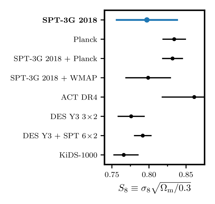
Bottom panel: A compilation of constraints using different cosmological data sets: SPT-3G 2018, Planck [1], WMAP [15], ACT DR4 [5], DES Y3 [52], DES Y3 + SPT [54], and KiDS-1000 [51]. Note that all constraints are produced assuming CDM. The central value of the SPT-3G constraint lies between those of low-redshift analyses and Planck.
We find the scalar spectral index of primordial fluctuations to be , which corresponds to a preference for . We note that when excising our measurement of the third acoustic peak of the temperature power spectrum, i.e. data at , we find . The corresponding five-dimensional parameter shift from the baseline result is a event, where denotes the number of standard deviations equivalent to the associated PTE for a Gaussian distribution. This is compatible with a statistical fluctuation and we therefore expect that the addition of more data to the subset, i.e. our baseline configuration with data at , yields constraints closer to the underlying mean. This matches what we observe when comparing to the tight constraints of Planck and WMAP [1, 55], which are enabled by the broad coverage of scales in space of satellite data; adding data at to the subset shifts our result towards these tight constraints.
For a less model-dependent check on our measurement at we compare our minimum-variance band powers to the Planck full-sky power spectrum. Given that both data sets are sample-variance-dominated on these angular scales, we assume that the SPT data are a subset of the Planck data; we use the difference of the SPT and Planck band power covariance matrices as the covariance of the difference between the two data sets. We report a PTE value of . This indicates that the two power spectrum measurements are in good agreement and we conclude that the effect the SPT-3G data at has on is not statistically anomalous.
| SPT-3G 2018 | SPT-3G 2018 + Planck | SPT-3G 2018 + WMAP | Planck | |
We find excellent agreement between cosmological constraints from SPT-3G 2018 and Planck data. For individual CDM parameters, all differences are . Comparing all five parameters constrained by the SPT data, we find , corresponding to a PTE value of . This indicates a high level of agreement between the two data sets. This is particularly striking given that SPT-3G and Planck constraints are effectively independent of one another, given the large amount of sky observed by Planck that is not observed by SPT and the different weighting of the data as well as the different weightings of the , , and spectra. Though we use Planck data to calibrate our power spectrum measurement, we marginalize over the temperature calibration and polarization efficiency in the likelihood analysis. Furthermore, as per §IV.4 we find that our cosmological results are robust when replacing the Planck-based prior on the optical depth to reionization with the result of Natale et al. [46]. The agreement between SPT-3G and Planck data is not only a strong argument for the consistency and robustness of both experiments’ cosmological results, but implies consistency of the CDM model across angular scales and temperature and polarization spectra.
We find acceptable agreement between constraints from SPT-3G 2018 and ACT DR4. Across the five CDM parameters constrained by the ground-based experiments, we find , which translates to a PTE value of . Interestingly, the largest difference is in , which controls the positions of acoustic peaks; CMB data constrain this parameter with great precision and SPT-3G 2018 yields a measurement. ACT data yield a value and larger than SPT-3G and Planck data, respectively. Aiola et al. [5] note an offset in the cosmological parameter constraints on and when comparing Planck and ACT results (also visible in Fig. 7). Due to the degeneracy of these parameters with , the observed offset between ACT and SPT-3G constraints is likely related and from a similar origin. Regardless, the multi-dimensional test indicates that the observed parameter shifts are compatible with statistical fluctuations.
We report joint constraints from SPT-3G 2018 and Planck data in Table 4 and find . This is a refinement of the Planck constraint on by . The precision measurement of the CMB anisotropies at small angular scales in temperature and polarization provided by SPT-3G shrinks the Planck posteriors by approximately for each CDM parameter. Across the six-dimensional parameter space we report a reduction of the allowed volume by a factor of ; for comparison, only adding the SPT data to Planck leads to a reduction of the allowed parameter volume by a factor of . Due to the excellent agreement of SPT and Planck data, the shift to central values of parameter constraints compared to Planck alone is small.
The SPT-3G 2018 data are in good agreement with WMAP and we report a PTE value for a five-dimensional parameter-space comparison of . Combining the SPT-3G and WMAP data yields constraints largely independent of Planck, which we list in Table 4. We report , which lies below the distance-ladder analysis of Riess et al. [47] and deepens the Hubble tension. We report a constraint on the combined structure growth parameter of , which is compatible with Planck, as well as DES Y3 and KiDS-1000 data and the SZ-cluster analysis of Bocquet et al. [53] within . [1, 51, 52]. The addition of the low power spectrum measurement of WMAP to SPT-3G data refines our constraint by . We report , which disfavors a scale-invariant Harrison-Zel’dovich spectrum at . For comparison, from WMAP data alone we infer , which is from unity; the addition of SPT data tightens the constraint derived from WMAP data alone by .
VI.2 Gravitational Lensing,
The lensing of CMB photons emitted at the surface of last scattering by intervening large scale structure causes a characteristic distortion of the CMB anisotropies leading to changes in the power spectrum: a smoothing of acoustic peaks and a transfer of power to the damping tail. Though the magnitude of this effect is derived from the values of cosmological parameters in the CDM model, marginalizing over the effect of lensing on the primary CMB power spectra assesses the compatibility of the data with the standard model [56, 57, 58]. Planck Collaboration et al. [1] find a preference for increased lensing at .
We marginalize over an artificial scaling of the lensing power spectrum that smears the primary CMB, , and report parameter constraints in Table 5. We find
| (13) |
which is compatible with the standard model prediction of unity at . Adding does not lead to a statistically significant improvement to the goodness-of-fit compared to CDM ().
| SPT-3G 2018 | SPT-3G 2018 + Planck | SPT-3G 2018 | SPT-3G 2018 + Planck | SPT-3G 2018 | SPT-3G 2018 + Planck | |
The SPT-3G 2018 band powers provide a sample-variance-limited measurement of the third and higher order acoustic peaks, which helps constrain cosmological parameters in this model. The constraint improves by for compared to as shown in Figure 9. Across all six dimensions, the allowed parameter volume shrinks by a factor of .
In this model the SPT-3G and Planck constraints slightly diverge. Planck data yield , which is away from our result. Nevertheless, comparing the two data sets across the full six-dimensional parameter space gives , which translates to a PTE value of and indicates that the parameter shifts are consistent with statistical fluctuations.
We report joint constraints from SPT-3G 2018 and Planck data in Table 5. We find , which is within of the standard model prediction. Adding SPT-3G to Planck data lowers the significance of the deviation from unity and constraints on other cosmological parameters shift closer to the Planck only CDM results. The width of the posterior shrinks by when adding SPT-3G to Planck data and the seven-dimensional allowed parameter volume decreases by a factor of .
We revisit the investigation of lensing convergence on the SPT-3G survey patch from Balkenhol et al. [3] using the complete SPT-3G 2018 data set. We analyze joint constraints from SPT-3G 2018 and Planck data in CDM foregoing the baseline Gaussian prior on . We adjust the sign of the definition in §III to match Motloch & Hu [59] and the appendix of Balkenhol et al. [3]. We find
| (14) |
While the sign matches the result of Balkenhol et al. [3], our central value is compatible with zero at . We conclude that this test provides no significant evidence that the SPT-3G survey field aligns with a local density anomaly.
VI.3 Effective Number of Neutrino Species,
Additional relativistic particles in the early universe, e.g., axion-like particles, hidden photons, gravitinos, massless Goldstone bosons, additional neutrino species, as well as other forms of energy injection imprint on the CMB power spectra. At the parameter level, this modifies the effective number of neutrino species, , which is in the standard model [60, 61, 62, 63, 64].
We report constraints on the CDM model in Table 5, finding
| (15) |
This result is compatible with the standard model prediction at . The best-fit CDM model does not improve on the good fit to the SPT-3G data achieved by CDM significantly ().
The addition of sample-variance-limited measurements of the damping tail of the power spectrum improves on the cosmological constraints achieved by SPT-3G 2018 in this model. As shown Figure 9, the posterior of tightens by when adding the SPT-3G 2018 band powers. The allowed volume across the full six dimensional parameter space shrinks by a factor of .
We find good agreement on between the SPT-3G and Planck data with the central values separated by . Comparing all six parameters simultaneously, we find , which translates to a PTE value of . The parameter constraints are compatible with statistical fluctuations.
We list joint constraints from SPT-3G 2018 and Planck in Table 5 and report . This constraint on the effective number of neutrino species is in excellent agreement with the standard model prediction of (). While the addition of the SPT-3G to the Planck data set only leads to a marginal improvement of the constraint (), the allowed seven-dimensional parameter volume is reduced by a factor of .
VI.4 Effective Number of Neutrino Species and Primordial Helium Abundance,
Varying alone assumes that any additional relativistic species present at recombination were also present at big-bang nucleosynthesis. By simultaneously marginalizing over the primordial helium abundance, , we remove this assumption and flexibly probe the relativistic energy density in the early universe [65, 63].
We present constraints from SPT-3G 2018 in Table 5. We report
| (16) | ||||
The central values of the and constraints are compatible with the standard model predictions at and , respectively. We report no significant improvement to the goodness-of-fit for this model over CDM ( for two additional parameters).
Comparing the determinants of the parameter covariances when using vs. data, we find that the allowed parameter volume is reduced by a factor of through the inclusion of temperature band powers. The and uncertainties shrink by and , respectively, which we show in Figure 9.
Again, we find good agreement between SPT-3G and Planck data in this model: across the full seven-dimensional parameter space we report , which translates to a PTE value of . The and constraints of the two data sets are compatible at and , respectively. We conclude that the differences in parameter constraints are compatible with statistical fluctuations.
Joint constraints from SPT-3G 2018 and Planck are given in Table 5. We report and . The central values of the joint SPT-3G and Planck and constraints lie within and of their standard model predictions, respectively, and improve on the Planck only results by and , respectively. Across the full eight-dimensional parameter space, the addition of SPT-3G to Planck data leads to a reduction of the allowed parameter volume by a factor of .
VI.5 Primordial Magnetic Fields

The presence of primordial magnetic fields (PMFs), i.e. magnetic fields prior to recombination, increases the inhomogeneity of the baryon density, . This so-called baryon clumping effect is parametrized by , such that corresponds to no PMFs. With other cosmological parameters fixed, increasing changes the width of the visibility function and shifts it to higher redshifts, i.e. recombination occurs sooner, which leads one to infer higher values of from CMB data [66, 67, 68, 17]. Because the distribution of baryons in the early universe is not known precisely, we use the three-zone toy model put forward by Jedamzik & Abel [66] and Jedamzik & Pogosian [68].
We list constraints on CDM+ from the SPT-3G 2018 data in Table 6 and show the marginalized one-dimensional posterior for in Figure 12. We find a 95% confidence upper limit of
| (17) |
The tight limit on the PMF-induced baryon clumping limits the possibility of resolving the Hubble tension through this model; we find , which remains below the distance-ladder analysis of Riess et al. [47]. We find no improvement to the goodness-of-fit for this model compared to CDM ().
| SPT-3G 2018 | SPT-3G 2018 + Planck | |
Measurements of the full power spectra are crucial in this model. Galli et al. [17] point out a degeneracy between and that prohibits meaningful constraints on if only or only power spectrum measurements are available (see Figure 6 therein). Therefore, while Galli et al. [17] report an effective non-constraint on using the SPT-3G 2018 data set of D21, the addition of data in this work allows for a meaningful constraint, which we visualize in Figure 9.
Due to the sensitivity of the constraint to the values inferred from temperature and polarization data we confirm that our result is consistent with expectations based on simulations. The upper limit we report for the data is within of what we infer from simulated band powers centered on .
We find good agreement between SPT-3G and Planck constraints in this model. Across the full seven-dimensional parameter space we report , which translates to a PTE value of . We report joint constraints from SPT-3G 2018 and Planck data on CDM+ in Table 6. We find a 95% confidence upper limit of . The addition of the SPT-3G data to Planck tightens the upper limit by and reduces the volume of the allowed parameter space by a factor of .
VII Conclusion
In this work, we present a measurement of the CMB temperature power spectrum using SPT-3G data recorded in 2018. The band powers are sample-variance-limited across the reported angular multipole range of . Together with the already published polarization data [D21] from the same observing season, this completes the SPT-3G 2018 data set. We analyze the internal consistency of the data using a variety of tools: null tests, difference spectra, complement spectra (across frequencies and spectrum types), MV comparisons, and parameter-level subset tests. We find good agreement across frequencies, spectrum types, and angular multipoles.
We present cosmological parameter constraints from the SPT-3G 2018 band powers. This is the first analysis using SPT-only measurements of all three primary CMB power spectra and the complete data set provides the strongest constraining power to date from SPT. The data are well fit by CDM with a PTE value of . We constrain the expansion rate today to , the combined structure growth parameter to , and find a preference for at . The addition of the SPT-3G temperature power spectrum measurement to the data improves cosmological parameter constraints by and reduces the allowed five-dimensional parameter volume by a factor of . We report excellent agreement between the SPT-3G and Planck data with deviations of for all cosmological parameters. Adding the SPT-3G band powers to the Planck primary power spectrum measurement leads to a reduction of the allowed six-dimensional parameter volume by a factor of .
We consider a series of extensions to the standard model, drawing on the following parameters: the strength of gravitational lensing affecting the primary CMB power spectra, , the effective number of neutrino species, , the primordial helium abundance, , and the baryon-clumping induced by primordial magnetic fields, . We do not find a preference for any of these extensions over the standard model. The addition of temperature data to power spectrum measurements leads to significant improvements on cosmological constraints. For CDM, CDM, and CDM, the posterior widths of extension parameters shrink by and the multidimensional allowed parameter volume decreases by factors of . In the case of primordial magnetic fields, the combination of temperature and polarization data is essential to break degeneracies between and [17]. We find a confidence upper limit on the PMF-induced baryon clumping of . Our findings reflect that joint analyses of power spectrum measurements yield a substantial increase in constraining power over alone; this approach is key to distinguishing between significant deviations from the standard model and statistical fluctuations and provides further ways to test the data for systematic effects.
The framework presented here will be used for on-going analyses of SPT-3G data recorded in the 2019 and 2020 observing seasons. These observations include measurements of the same survey field used here, but achieve a map noise smaller. Moreover, extended survey data from these seasons cover an additional , reducing sample variance and improving measurements of the power spectrum on large angular scales. The combined SPT-3G measurements presented in this work represent a significant improvement for cosmological constraints from ground-based CMB data, and are an important demonstration for future experiments, such as CMB-S4 [69].
Acknowledgements.
We thank Karsten Jedamzik and Levon Pogosian for their help with models featuring baryon clumping due to primordial magnetic fields. The South Pole Telescope program is supported by the National Science Foundation (NSF) through the awards OPP-1852617 and OPP-2147371. Partial support is also provided by the Kavli Institute of Cosmological Physics at the University of Chicago. Argonne National Laboratory’s work was supported by the U.S. Department of Energy, Office of High Energy Physics, under Contract No. DE-AC02-06CH11357. Work at Fermi National Accelerator Laboratory, a DOE-OS, HEP User Facility managed by the Fermi Research Alliance, LLC, was supported under Contract No. DE-AC02-07CH11359. The Cardiff authors acknowledge support from the UK Science and Technologies Facilities Council (STFC). The IAP authors acknowledge support from the Centre National d’Études Spatiales (CNES). This project has received funding from the European Research Council (ERC) under the European Union’s Horizon 2020 research and innovation programme (grant agreement No 101001897). This research used resources of the IN2P3 Computer Center (http://cc.in2p3.fr). M.A. and J.V. acknowledge support from the Center for AstroPhysical Surveys at the National Center for Supercomputing Applications in Urbana, IL. J.V. acknowledges support from the Sloan Foundation. K.F. acknowledges support from the Department of Energy Office of Science Graduate Student Research (SCGSR) Program. The Melbourne authors acknowledge support from the Australian Research Council’s Discovery Project scheme (No. DP210102386). L.B. acknowledges support from the Albert Shimmins Fund. The McGill authors acknowledge funding from the Natural Sciences and Engineering Research Council of Canada, Canadian Institute for Advanced Research, and the Fonds de recherche du Québec Nature et technologies. The UCLA and MSU authors acknowledge support from NSF AST-1716965 and CSSI-1835865. A.S.M. is supported by the MSSL STFC Consolidated Grant. This research was done using resources provided by the Open Science Grid [70, 71], which is supported by the NSF Award No. 1148698, and the U.S. Department of Energy’s Office of Science. Some of the results in this paper have been derived using the healpy and HEALPix121212http://healpix.sf.net/ packages [72, 73]. The data analysis pipeline also uses the scientific python stack [74, 75, 76].References
- Planck Collaboration et al. [2020a] Planck Collaboration, Aghanim, N., Akrami, Y., et al. Planck 2018 results. VI. Cosmological parameters. 2020a, A&A, 641, A6, doi: 10.1051/0004-6361/201833910
- Dutcher et al. [2021] Dutcher, D., Balkenhol, L., Ade, P. A. R., et al. Measurements of the E -mode polarization and temperature-E -mode correlation of the CMB from SPT-3G 2018 data. 2021, Phys. Rev. D, 104, 022003, doi: 10.1103/PhysRevD.104.022003
- Balkenhol et al. [2021] Balkenhol, L., Dutcher, D., Ade, P. A. R., et al. Constraints on CDM extensions from the SPT-3G 2018 E E and T E power spectra. 2021, Phys. Rev. D, 104, 083509, doi: 10.1103/PhysRevD.104.083509
- Choi et al. [2020] Choi, S. K., Hasselfield, M., Ho, S.-P. P., et al. The Atacama Cosmology Telescope: A Measurement of the Cosmic Microwave Background Power Spectra at 98 and 150 GHz. 2020, arXiv e-prints, arXiv:2007.07289. https://arxiv.org/abs/2007.07289
- Aiola et al. [2020] Aiola, S., Calabrese, E., Maurin, L., et al. The Atacama Cosmology Telescope: DR4 Maps and Cosmological Parameters. 2020, arXiv e-prints, arXiv:2007.07288. https://arxiv.org/abs/2007.07288
- Carlstrom et al. [2011] Carlstrom, J. E., Ade, P. A. R., Aird, K. A., et al. The 10 Meter South Pole Telescope. 2011, PASP, 123, 568, doi: 10.1086/659879
- Kosowsky [2003] Kosowsky, A. The Atacama Cosmology Telescope. 2003, in the proceedings of the workshop on “The Cosmic Microwave Background and its Polarization,” New Astronomy Reviews, ed. S. Hanany & K. A. Olive (Elsevier)
- Kermish et al. [2012] Kermish, Z. D., Ade, P., Anthony, A., et al. The POLARBEAR experiment. 2012, in Society of Photo-Optical Instrumentation Engineers (SPIE) Conference Series, Vol. 8452, Millimeter, Submillimeter, and Far-Infrared Detectors and Instrumentation for Astronomy VI, ed. W. S. Holland & J. Zmuidzinas, 84521C, doi: 10.1117/12.926354
- Keating et al. [2003] Keating, B. G., Ade, P. A. R., Bock, J. J., Hivon, E., Holzapfel, W. L., Lange, A. E., Nguyen, H., & Yoon, K. BICEP: a large angular scale CMB polarimeter. 2003, in Polarimetry in Astronomy. Edited by Silvano Fineschi. Proceedings of the SPIE, Volume 4843., 284–295
- Staniszewski et al. [2012] Staniszewski, Z., Aikin, R. W., Amiri, M., et al. The Keck Array: A Multi Camera CMB Polarimeter at the South Pole. 2012, Journal of Low Temperature Physics, 167, 827, doi: 10.1007/s10909-012-0510-1
- Planck Collaboration et al. [2020b] Planck Collaboration, Aghanim, N., Akrami, Y., et al. Planck 2018 results. V. CMB power spectra and likelihoods. 2020b, A&A, 641, A5, doi: 10.1051/0004-6361/201936386
- Galli et al. [2014] Galli, S., Benabed, K., Bouchet, F., Cardoso, J.-F., Elsner, F., Hivon, E., Mangilli, A., Prunet, S., & Wandelt, B. CMB polarization can constrain cosmology better than CMB temperature. 2014, Phys. Rev. D, 90, 063504, doi: 10.1103/PhysRevD.90.063504
- Reichardt et al. [2009] Reichardt, C. L., Ade, P. A. R., Bock, J. J., et al. High-Resolution CMB Power Spectrum from the Complete ACBAR Data Set. 2009, Astrophys. J. , 694, 1200, doi: 10.1088/0004-637X/694/2/1200
- Das et al. [2011] Das, S., Marriage, T. A., Ade, P. A. R., et al. The Atacama Cosmology Telescope: A Measurement of the Cosmic Microwave Background Power Spectrum at 148 and 218 GHz from the 2008 Southern Survey. 2011, Astrophys. J. , 729, 62, doi: 10.1088/0004-637X/729/1/62
- Bennett et al. [2013] Bennett, C. L., Larson, D., Weiland, J. L., et al. Nine-year Wilkinson Microwave Anisotropy Probe (WMAP) Observations: Final Maps and Results. 2013, Ap. J. Suppl. , 208, 20, doi: 10.1088/0067-0049/208/2/20
- Story et al. [2013] Story, K. T., Reichardt, C. L., Hou, Z., et al. A Measurement of the Cosmic Microwave Background Damping Tail from the 2500-Square-Degree SPT-SZ Survey. 2013, Astrophys. J. , 779, 86, doi: 10.1088/0004-637X/779/1/86
- Galli et al. [2022] Galli, S., Pogosian, L., Jedamzik, K., & Balkenhol, L. Consistency of Planck, ACT, and SPT constraints on magnetically assisted recombination and forecasts for future experiments. 2022, Phys. Rev. D, 105, 023513, doi: 10.1103/PhysRevD.105.023513
- Benson et al. [2014] Benson, B. A., Ade, P. A. R., Ahmed, Z., et al. SPT-3G: A Next-Generation Cosmic Microwave Background Polarization Experiment on the South Pole Telescope. 2014, in Proc. SPIE, Vol. 9153, Millimeter, Submillimeter, and Far-Infrared Detectors and Instrumentation for Astronomy VII, 91531P, doi: 10.1117/12.2057305
- Sobrin et al. [2022] Sobrin, J. A., Anderson, A. J., Bender, A. N., et al. The Design and Integrated Performance of SPT-3G. 2022, The Astrophysical Journal Supplement Series, 258, 42, doi: 10.3847/1538-4365/ac374f
- Hivon et al. [2002] Hivon, E., Górski, K. M., Netterfield, C. B., Crill, B. P., Prunet, S., & Hansen, F. MASTER of the Cosmic Microwave Background Anisotropy Power Spectrum: A Fast Method for Statistical Analysis of Large and Complex Cosmic Microwave Background Data Sets. 2002, Astrophys. J. , 567, 2, doi: 10.1086/338126
- Lewis & Bridle [2002] Lewis, A., & Bridle, S. Cosmological parameters from CMB and other data: A Monte Carlo approach. 2002, Phys. Rev. D, 66, 103511
- Lewis et al. [2000] Lewis, A., Challinor, A., & Lasenby, A. Efficient Computation of Cosmic Microwave Background Anisotropies in Closed Friedmann-Robertson-Walker Models. 2000, Astrophys. J. , 538, 473, doi: 10.1086/309179
- Spurio Mancini et al. [2022] Spurio Mancini, A., Piras, D., Alsing, J., Joachimi, B., & Hobson, M. P. COSMOPOWER: emulating cosmological power spectra for accelerated Bayesian inference from next-generation surveys. 2022, MNRAS, 511, 1771, doi: 10.1093/mnras/stac064
- Hu & Sugiyama [1996] Hu, W., & Sugiyama, N. Small-Scale Cosmological Perturbations: an Analytic Approach. 1996, Astrophys. J. , 471, 542, doi: 10.1086/177989
- Fendt & Wandelt [2007] Fendt, W. A., & Wandelt, B. D. Pico: Parameters for the Impatient Cosmologist. 2007, Astrophys. J. , 654, 2, doi: 10.1086/508342
- Blas et al. [2011] Blas, D., Lesgourgues, J., & Tram, T. The Cosmic Linear Anisotropy Solving System (CLASS). Part II: Approximation schemes. 2011, J. of Cosm. & Astropart. Phys., 2011, 034, doi: 10.1088/1475-7516/2011/07/034
- Hill et al. [2022] Hill, J. C., Calabrese, E., Aiola, S., et al. Atacama Cosmology Telescope: Constraints on prerecombination early dark energy. 2022, Phys. Rev. D, 105, 123536, doi: 10.1103/PhysRevD.105.123536
- Jeong et al. [2014] Jeong, D., Chluba, J., Dai, L., Kamionkowski, M., & Wang, X. Effect of aberration on partial-sky measurements of the cosmic microwave background temperature power spectrum. 2014, Phys. Rev. D, 89, 023003, doi: 10.1103/PhysRevD.89.023003
- Manzotti et al. [2014] Manzotti, A., Hu, W., & Benoit-Lévy, A. Super-sample CMB lensing. 2014, Phys. Rev. D, 90, 023003, doi: 10.1103/PhysRevD.90.023003
- Reichardt et al. [2020] Reichardt, C. L., Patil, S., Ade, P. A. R., et al. An Improved Measurement of the Secondary Cosmic Microwave Background Anisotropies from the SPT-SZ + SPTpol Surveys. 2020, arXiv e-prints, arXiv:2002.06197. https://arxiv.org/abs/2002.06197
- George et al. [2015] George, E. M., Reichardt, C. L., Aird, K. A., et al. A Measurement of Secondary Cosmic Microwave Background Anisotropies from the 2500-Square-degree SPT-SZ Survey. 2015, Astrophys. J. , 799, 177, doi: 10.1088/0004-637X/799/2/177
- Dunkley et al. [2013] Dunkley, J., Calabrese, E., Sievers, J., et al. The Atacama Cosmology Telescope: likelihood for small-scale CMB data. 2013, J. of Cosm. & Astropart. Phys., 7, 25, doi: 10.1088/1475-7516/2013/07/025
- De Zotti et al. [2005] De Zotti, G., Ricci, R., Mesa, D., Silva, L., Mazzotta, P., Toffolatti, L., & González-Nuevo, J. Predictions for high-frequency radio surveys of extragalactic sources. 2005, A&A, 431, 893, doi: 10.1051/0004-6361:20042108
- Fixsen [2009] Fixsen, D. J. The Temperature of the Cosmic Microwave Background. 2009, Astrophys. J. , 707, 916, doi: 10.1088/0004-637X/707/2/916
- Addison et al. [2012] Addison, G. E., Dunkley, J., Hajian, A., et al. Power-law Template for Infrared Point-source Clustering. 2012, Astrophys. J. , 752, 120, doi: 10.1088/0004-637X/752/2/120
- Shaw et al. [2010] Shaw, L. D., Nagai, D., Bhattacharya, S., & Lau, E. T. Impact of Cluster Physics on the Sunyaev-Zel’dovich Power Spectrum. 2010, Astrophys. J. , 725, 1452, doi: 10.1088/0004-637X/725/2/1452
- Shaw et al. [2012] Shaw, L. D., Rudd, D. H., & Nagai, D. Deconstructing the Kinetic SZ Power Spectrum. 2012, Astrophys. J. , 756, 15, doi: 10.1088/0004-637X/756/1/15
- Zahn et al. [2012] Zahn, O., Reichardt, C. L., Shaw, L., et al. Cosmic Microwave Background Constraints on the Duration and Timing of Reionization from the South Pole Telescope. 2012, Astrophys. J. , 756, 65, doi: 10.1088/0004-637X/756/1/65
- Planck Collaboration et al. [2014] Planck Collaboration, Ade, P. A. R., Aghanim, N., Armitage-Caplan, C., Arnaud, M., Ashdown, M., Atrio-Barandela, F., Aumont, J., Baccigalupi, C., Banday, A. J., & et al. Planck 2013 results. XV. CMB power spectra and likelihood. 2014, A&A, 571, A15, doi: 10.1051/0004-6361/201321573
- Dunn [1961] Dunn, O. J. Multiple Comparisons Among Means. 1961, American Statistical Association, 52
- Planck Collaboration et al. [2016] Planck Collaboration, Aghanim, N., Arnaud, M., Ashdown, M., Aumont, J., Baccigalupi, C., Banday, A. J., Barreiro, R. B., Bartlett, J. G., Bartolo, N., & et al. Planck 2015 results. XI. CMB power spectra, likelihoods, and robustness of parameters. 2016, A&A, 594, A11, doi: 10.1051/0004-6361/201526926
- Mocanu et al. [2019] Mocanu, L. M., Crawford, T. M., Aylor, K., et al. Consistency of cosmic microwave background temperature measurements in three frequency bands in the 2500-square-degree SPT-SZ survey. 2019, J. of Cosm. & Astropart. Phys., 2019, 038, doi: 10.1088/1475-7516/2019/07/038
- Gratton & Challinor [2019] Gratton, S., & Challinor, A. Understanding parameter differences between analyses employing nested data subsets. 2019, arXiv e-prints, arXiv:1911.07754. https://arxiv.org/abs/1911.07754
- Henning et al. [2018] Henning, J. W., Sayre, J. T., Reichardt, C. L., et al. Measurements of the Temperature and E-mode Polarization of the CMB from 500 Square Degrees of SPTpol Data. 2018, Astrophys. J. , 852, 97, doi: 10.3847/1538-4357/aa9ff4
- Adachi et al. [2020] Adachi, S., Aguilar Faúndez, M. A. O., Arnold, K., et al. A measurement of the CMB E-mode angular power spectrum at subdegree scales from 670 square degrees of POLARBEAR data. 2020, arXiv e-prints, arXiv:2005.06168. https://arxiv.org/abs/2005.06168
- Natale et al. [2020] Natale, U., Pagano, L., Lattanzi, M., Migliaccio, M., Colombo, L. P., Gruppuso, A., Natoli, P., & Polenta, G. A novel CMB polarization likelihood package for large angular scales built from combined WMAP and Planck LFI legacy maps. 2020, arXiv e-prints, arXiv:2005.05600. https://arxiv.org/abs/2005.05600
- Riess et al. [2022] Riess, A. G., Yuan, W., Macri, L. M., et al. A Comprehensive Measurement of the Local Value of the Hubble Constant with 1 km s-1 Mpc-1 Uncertainty from the Hubble Space Telescope and the SH0ES Team. 2022, Ap. J. Lett. , 934, L7, doi: 10.3847/2041-8213/ac5c5b
- Freedman et al. [2019] Freedman, W. L., Madore, B. F., Hatt, D., Hoyt, T. J., Jang, I.-S., Beaton, R. L., Burns, C. R., Lee, M. G., Monson, A. J., Neeley, J. R., Phillips, M. M., Rich, J. A., & Seibert, M. The Carnegie-Chicago Hubble Program. VIII. An Independent Determination of the Hubble Constant Based on the Tip of the Red Giant Branch. 2019, arXiv e-prints, arXiv:1907.05922. https://arxiv.org/abs/1907.05922
- Wong et al. [2020] Wong, K. C., Suyu, S. H., Chen, G. C. F., et al. H0LiCOW XIII. A 2.4% measurement of H0 from lensed quasars: 5.3 tension between early and late-Universe probes. 2020, MNRAS, doi: 10.1093/mnras/stz3094
- Birrer et al. [2020] Birrer, S., Shajib, A. J., Galan, A., et al. TDCOSMO IV: Hierarchical time-delay cosmography – joint inference of the Hubble constant and galaxy density profiles. 2020, arXiv e-prints, arXiv:2007.02941. https://arxiv.org/abs/2007.02941
- Heymans et al. [2020] Heymans, C., Tröster, T., Asgari, M., et al. KiDS-1000 Cosmology: Multi-probe weak gravitational lensing and spectroscopic galaxy clustering constraints. 2020, arXiv e-prints, arXiv:2007.15632. https://arxiv.org/abs/2007.15632
- Abbott et al. [2022a] Abbott, T. M. C., Aguena, M., Alarcon, A., et al. Dark Energy Survey Year 3 results: Cosmological constraints from galaxy clustering and weak lensing. 2022a, Phys. Rev. D, 105, 023520, doi: 10.1103/PhysRevD.105.023520
- Bocquet et al. [2019] Bocquet, S., Dietrich, J. P., Schrabback, T., et al. Cluster Cosmology Constraints from the 2500 deg2 SPT-SZ Survey: Inclusion of Weak Gravitational Lensing Data from Magellan and the Hubble Space Telescope. 2019, Astrophys. J. , 878, 55, doi: 10.3847/1538-4357/ab1f10
- Abbott et al. [2022b] Abbott, T. M. C., Aguena, M., Alarcon, A., et al. Joint analysis of DES Year 3 data and CMB lensing from SPT and Planck III: Combined cosmological constraints. 2022b, arXiv e-prints, arXiv:2206.10824. https://arxiv.org/abs/2206.10824
- Hinshaw et al. [2013] Hinshaw, G., Larson, D., Komatsu, E., et al. Nine-year Wilkinson Microwave Anisotropy Probe (WMAP) Observations: Cosmological Parameter Results. 2013, Ap. J. Suppl. , 208, 19, doi: 10.1088/0067-0049/208/2/19
- Seljak [1996] Seljak, U. Gravitational Lensing Effect on Cosmic Microwave Background Anisotropies: A Power Spectrum Approach. 1996, Astrophys. J. , 463, 1, doi: 10.1086/177218
- Lewis & Challinor [2006] Lewis, A., & Challinor, A. Weak gravitational lensing of the CMB. 2006, Phys. Rep., 429, 1, doi: 10.1016/j.physrep.2006.03.002
- Calabrese et al. [2008] Calabrese, E., Slosar, A., Melchiorri, A., Smoot, G. F., & Zahn, O. Cosmic microwave weak lensing data as a test for the dark universe. 2008, Phys. Rev. D, 77, 123531, doi: 10.1103/PhysRevD.77.123531
- Motloch & Hu [2019] Motloch, P., & Hu, W. Lensing covariance on cut sky and SPT-Planck lensing tensions. 2019, Phys. Rev. D, 99, 023506, doi: 10.1103/PhysRevD.99.023506
- Froustey et al. [2020] Froustey, J., Pitrou, C., & Volpe, M. C. Neutrino decoupling including flavour oscillations and primordial nucleosynthesis. 2020, J. of Cosm. & Astropart. Phys., 2020, 015, doi: 10.1088/1475-7516/2020/12/015
- Bennett et al. [2020] Bennett, J. J., Buldgen, G., de Salas, P. F., Drewes, M., Gariazzo, S., Pastor, S., & Wong, Y. Y. Y. Towards a precision calculation of in the Standard Model II: Neutrino decoupling in the presence of flavour oscillations and finite-temperature QED. 2020, arXiv e-prints, arXiv:2012.02726. https://arxiv.org/abs/2012.02726
- Brust et al. [2013] Brust, C., Kaplan, D. E., & Walters, M. T. New light species and the CMB. 2013, Journal of High Energy Physics, 2013, 58, doi: 10.1007/JHEP12(2013)058
- Group et al. [2020] Group, P. D., Zyla, P. A., Barnett, R. M., et al. Review of Particle Physics. 2020, Progress of Theoretical and Experimental Physics, 2020, doi: 10.1093/ptep/ptaa104
- Abazajian et al. [2016] Abazajian, K. N., Adshead, P., Ahmed, Z., et al. CMB-S4 Science Book, First Edition. 2016, ArXiv e-prints. https://arxiv.org/abs/1610.02743
- Cyburt et al. [2016] Cyburt, R. H., Fields, B. D., Olive, K. A., & Yeh, T.-H. Big bang nucleosynthesis: Present status. 2016, Reviews of Modern Physics, 88, 015004, doi: 10.1103/RevModPhys.88.015004
- Jedamzik & Abel [2013] Jedamzik, K., & Abel, T. Small-scale primordial magnetic fields and anisotropies in the cosmic microwave background radiation. 2013, Journal of Cosmology and Astroparticle Physics, 2013, 050, doi: 10.1088/1475-7516/2013/10/050
- Jedamzik & Saveliev [2019] Jedamzik, K., & Saveliev, A. Stringent Limit on Primordial Magnetic Fields from the Cosmic Microwave Background Radiation. 2019, Phys. Rev. Lett. , 123, 021301, doi: 10.1103/PhysRevLett.123.021301
- Jedamzik & Pogosian [2020] Jedamzik, K., & Pogosian, L. Relieving the Hubble Tension with Primordial Magnetic Fields. 2020, Phys. Rev. Lett. , 125, 181302, doi: 10.1103/PhysRevLett.125.181302
- CMB-S4 Collaboration et al. [2019] CMB-S4 Collaboration, Abazajian, K., Addison, G., Adshead, P., Ahmed, Z., Allen, S. W., Alonso, D., Alvarez, M., Anderson, A., Arnold, K. S., Baccigalupi, C., & et al. CMB-S4 Science Case, Reference Design, and Project Plan. 2019, arXiv e-prints, arXiv:1907.04473. https://arxiv.org/abs/1907.04473
- Pordes et al. [2007] Pordes, R., et al. The Open Science Grid. 2007, J. Phys. Conf. Ser., 78, 012057, doi: 10.1088/1742-6596/78/1/012057
- Sfiligoi et al. [2009] Sfiligoi, I., Bradley, D. C., Holzman, B., Mhashilkar, P., Padhi, S., & Wurthwein, F. The Pilot Way to Grid Resources Using glideinWMS. 2009, in 2, Vol. 2, 2009 WRI World Congress on Computer Science and Information Engineering, 428–432, doi: 10.1109/CSIE.2009.950
- Górski et al. [2005] Górski, K. M., Hivon, E., Banday, A. J., Wandelt, B. D., Hansen, F. K., Reinecke, M., & Bartelmann, M. HEALPix: A Framework for High-Resolution Discretization and Fast Analysis of Data Distributed on the Sphere. 2005, Astrophys. J. , 622, 759, doi: 10.1086/427976
- Zonca et al. [2019] Zonca, A., Singer, L., Lenz, D., Reinecke, M., Rosset, C., Hivon, E., & Gorski, K. healpy: equal area pixelization and spherical harmonics transforms for data on the sphere in Python. 2019, Journal of Open Source Software, 4, 1298, doi: 10.21105/joss.01298
- Hunter [2007] Hunter, J. D. Matplotlib: A 2D graphics environment. 2007, Computing In Science & Engineering, 9, 90, doi: 10.1109/MCSE.2007.55
- Jones et al. [2001] Jones, E., Oliphant, T., Peterson, P., et al. 2001, SciPy: Open source scientific tools for Python. http://www.scipy.org/
- van der Walt et al. [2011] van der Walt, S., Colbert, S., & Varoquaux, G. The NumPy Array: A Structure for Efficient Numerical Computation. 2011, Computing in Science Engineering, 13, 22, doi: 10.1109/MCSE.2011.37
- Lane [1998] Lane, A. P. Submillimeter Transmission at South Pole. 1998, in ASP Conf. Ser. 141, Vol. 141, Astrophysics from Antarctica, ed. G. Novak & R. H. Landsberg (San Francisco: ASP), 289
- Pardo et al. [2001] Pardo, J. R., Cernicharo, J., & Serabyn, E. Atmospheric transmission at microwaves (ATM): an improved model for millimeter/submillimeter applications. 2001, IEEE Transactions on Antennas and Propagation, 49, 1683, doi: 10.1109/8.982447
- Planck Collaboration et al. [2020c] Planck Collaboration, Aghanim, N., Akrami, Y., et al. Planck 2018 results. III. High Frequency Instrument data processing and frequency maps. 2020c, A&A, 641, A3, doi: 10.1051/0004-6361/201832909
Appendix
.1 Updates to the Polarization Analysis Pipeline
We make two key updates to the analysis of the spectra from D21, which primarily update the covariance matrix. First, we account for correlated noise across frequencies. Extending the work in D21, we take the difference between two half-depth coadded maps at different frequencies. We divide the power spectrum of this difference map by the square root of the product of the power spectra of the corresponding auto-frequency noise spectra. This yields an estimate of the correlation coefficient of the noise between two frequency channels. We find that for intensity the and channels, as well as the and channels, are moderately correlated with at and at . The and channels are highly correlated with at and at . This correlation is high compared to past and contemporary ground-based CMB experiments, due to the novel trichoic architecture of SPT-3G pixels [19]. The behaviour with matches the expectation that only atmospheric noise is correlated across frequencies, not instrumental noise. The different degrees of correlation are a consequence of a water emission line at and an oxygen line at [77, 78]. We use the correlation coefficients derived in this way to update the noise model in the covariance calculation (see §IVH in D21 for details). We detect no correlated noise across frequencies in polarization or correlated noise between temperature and polarization.
Second, we use a series of simulations to update the mode-coupling model in the covariance calculation. The Lambert azimuthal equal-area projection does not preserve angles and leads to increasing bin-to-bin correlations at high . For each simulation, we generate a CMB-only HEALPix sky, mask the map using the data apodization mask, and project the curved-sky map into a flat-sky map. We estimate the correlation matrix using the scatter of the power spectra of the flat-sky maps. The recovered correlation structure matches the data well and is less noisy than the data estimate due to the increased number of independent realizations. Following D21, we fit second-order polynomials to band-diagonal elements of the correlation estimate from simulations and use these fits in the data correlation matrix. While in principle filtering effects not captured by these simulations lead to off-diagonal elements in the covariance matrix, the correlation structure of the data is completely dominated by the flat-sky projection.
We compare parameter constraints from the original likelihood to the updated version in Table 7 and Figure 13. The central values of cosmological parameter constraints shift by less than the size of the new error bars. The parameter uncertainties generally widen with the updated covariance, by at most for . The addition of data to the updated covariance allows for as good as or better parameter constraints than reported in D21.

| SPT-3G 2018 (Original) | SPT-3G 2018 (Updated) | |
.2 Baseline Priors
We present the baseline priors used in the likelihood analysis and the best-fit values of nuisance parameters in CDM in Table 8.
We briefly present updates made to the galactic dust prior calculation of D21 here. We model the spectral dependence of galactic dust using a modified black-body spectrum and retain the angular dependence of D21, i.e. using a power law. The spectra are normalized at and . We fit combinations of the cross-spectra of the , , , and Planck PR3 half-mission maps [79] calculated on the SPT-3G survey field to the best-fit Planck CMB spectrum plus galactic dust and extragalactic foregrounds. We ensure the resulting constraints on the galactic dust parameters are robust with respect to the modelling of extragalactic foregrounds and the bin width of the cross-spectrum band powers. We conservatively widen the constraints the data provide on the galactic dust amplitudes by a factor of three before adopting them as priors in our cosmological analysis. The baseline priors on galactic dust are listed in Table 8.
| Parameter | Prior | Description |
| General | ||
| Optical depth to reionization | ||
| Super-sample lensing convergence | ||
| Temperature | ||
| Galactic cirrus amplitude | ||
| Galactic cirrus power law index | ||
| Galactic cirrus spectral index | ||
| Poisson power for | ||
| Poisson power for | ||
| Poisson power for | ||
| Poisson power for | ||
| Poisson power for | ||
| Poisson power for | ||
| CIB clustering amplitude | ||
| CIB clustering spectral index | ||
| tSZ amplitude | ||
| tSZ-CIB correlation | ||
| kSZ amplitude | ||
| Polarization | ||
| Poisson power for | ||
| Poisson power for | ||
| Poisson power for | ||
| Poisson power for | ||
| Poisson power for | ||
| Poisson power for | ||
| amplitude of polarized galactic dust | ||
| power law index of polarized galactic dust | ||
| spectral index of polarized galactic dust | ||
| amplitude of polarized galactic dust | ||
| power law index of polarized galactic dust | ||
| spectral index of polarized galactic dust | ||
| Calibration | ||
| Temperature calibration at | ||
| Temperature calibration at | ||
| Temperature calibration at | ||
| Polarization calibration at | ||
| Polarization calibration at | ||
| Polarization calibration at | ||
.3 Multifrequency Band Powers
| Range | |||||||||||||
| 750 – 800 | 775 | ||||||||||||
| 800 – 850 | 825 | ||||||||||||
| 850 – 900 | 874 | ||||||||||||
| 900 – 950 | 925 | ||||||||||||
| 950 – 1000 | 974 | ||||||||||||
| 1000 – 1050 | 1024 | ||||||||||||
| 1050 – 1100 | 1074 | ||||||||||||
| 1100 – 1150 | 1124 | ||||||||||||
| 1150 – 1200 | 1174 | ||||||||||||
| 1200 – 1250 | 1224 | ||||||||||||
| 1250 – 1300 | 1274 | ||||||||||||
| 1300 – 1350 | 1324 | ||||||||||||
| 1350 – 1400 | 1374 | ||||||||||||
| 1400 – 1450 | 1424 | ||||||||||||
| 1450 – 1500 | 1474 | ||||||||||||
| 1500 – 1550 | 1524 | ||||||||||||
| 1550 – 1600 | 1574 | ||||||||||||
| 1600 – 1650 | 1624 | ||||||||||||
| 1650 – 1700 | 1674 | ||||||||||||
| 1700 – 1750 | 1724 | ||||||||||||
| 1750 – 1800 | 1775 | ||||||||||||
| 1800 – 1850 | 1824 | ||||||||||||
| 1850 – 1900 | 1874 | ||||||||||||
| 1900 – 1950 | 1925 | ||||||||||||
| 1950 – 2000 | 1974 | ||||||||||||
| 2000 – 2100 | 2051 | ||||||||||||
| 2100 – 2200 | 2152 | ||||||||||||
| 2200 – 2300 | 2250 | ||||||||||||
| 2300 – 2400 | 2350 | ||||||||||||
| 2400 – 2500 | 2451 | ||||||||||||
| 2500 – 2600 | 2550 | ||||||||||||
| 2600 – 2700 | 2649 | ||||||||||||
| 2700 – 2800 | 2750 | ||||||||||||
| 2800 – 2900 | 2850 | ||||||||||||
| 2900 – 3000 | 2947 | ||||||||||||
| Range | |||||||||||||
| 300 – 350 | 326 | ||||||||||||
| 350 – 400 | 375 | ||||||||||||
| 400 – 450 | 425 | ||||||||||||
| 450 – 500 | 475 | ||||||||||||
| 500 – 550 | 525 | ||||||||||||
| 550 – 600 | 575 | ||||||||||||
| 600 – 650 | 625 | ||||||||||||
| 650 – 700 | 674 | ||||||||||||
| 700 – 750 | 725 | ||||||||||||
| 750 – 800 | 774 | ||||||||||||
| 800 – 850 | 824 | ||||||||||||
| 850 – 900 | 874 | ||||||||||||
| 900 – 950 | 924 | ||||||||||||
| 950 – 1000 | 974 | ||||||||||||
| 1000 – 1050 | 1024 | ||||||||||||
| 1050 – 1100 | 1074 | ||||||||||||
| 1100 – 1150 | 1124 | ||||||||||||
| 1150 – 1200 | 1174 | ||||||||||||
| 1200 – 1250 | 1224 | ||||||||||||
| 1250 – 1300 | 1274 | ||||||||||||
| 1300 – 1350 | 1324 | ||||||||||||
| 1350 – 1400 | 1374 | ||||||||||||
| 1400 – 1450 | 1424 | ||||||||||||
| 1450 – 1500 | 1474 | ||||||||||||
| 1500 – 1550 | 1524 | ||||||||||||
| 1550 – 1600 | 1574 | ||||||||||||
| 1600 – 1650 | 1624 | ||||||||||||
| 1650 – 1700 | 1674 | ||||||||||||
| 1700 – 1750 | 1724 | ||||||||||||
| 1750 – 1800 | 1775 | ||||||||||||
| 1800 – 1850 | 1824 | ||||||||||||
| 1850 – 1900 | 1874 | ||||||||||||
| 1900 – 1950 | 1924 | ||||||||||||
| 1950 – 2000 | 1975 | ||||||||||||
| 2000 – 2100 | 2050 | ||||||||||||
| 2100 – 2200 | 2150 | ||||||||||||
| 2200 – 2300 | 2250 | ||||||||||||
| 2300 – 2400 | 2350 | ||||||||||||
| 2400 – 2500 | 2450 | ||||||||||||
| 2500 – 2600 | 2550 | ||||||||||||
| 2600 – 2700 | 2649 | ||||||||||||
| 2700 – 2800 | 2749 | ||||||||||||
| 2800 – 2900 | 2849 | ||||||||||||
| 2900 – 3000 | 2946 | ||||||||||||
| Range | |||||||||||||
| 300 – 350 | 325 | ||||||||||||
| 350 – 400 | 375 | ||||||||||||
| 400 – 450 | 425 | ||||||||||||
| 450 – 500 | 475 | ||||||||||||
| 500 – 550 | 524 | ||||||||||||
| 550 – 600 | 575 | ||||||||||||
| 600 – 650 | 624 | ||||||||||||
| 650 – 700 | 674 | ||||||||||||
| 700 – 750 | 725 | ||||||||||||
| 750 – 800 | 774 | ||||||||||||
| 800 – 850 | 824 | ||||||||||||
| 850 – 900 | 874 | ||||||||||||
| 900 – 950 | 924 | ||||||||||||
| 950 – 1000 | 974 | ||||||||||||
| 1000 – 1050 | 1024 | ||||||||||||
| 1050 – 1100 | 1075 | ||||||||||||
| 1100 – 1150 | 1124 | ||||||||||||
| 1150 – 1200 | 1174 | ||||||||||||
| 1200 – 1250 | 1224 | ||||||||||||
| 1250 – 1300 | 1275 | ||||||||||||
| 1300 – 1350 | 1325 | ||||||||||||
| 1350 – 1400 | 1374 | ||||||||||||
| 1400 – 1450 | 1424 | ||||||||||||
| 1450 – 1500 | 1474 | ||||||||||||
| 1500 – 1550 | 1524 | ||||||||||||
| 1550 – 1600 | 1574 | ||||||||||||
| 1600 – 1650 | 1624 | ||||||||||||
| 1650 – 1700 | 1674 | ||||||||||||
| 1700 – 1750 | 1724 | ||||||||||||
| 1750 – 1800 | 1775 | ||||||||||||
| 1800 – 1850 | 1825 | ||||||||||||
| 1850 – 1900 | 1874 | ||||||||||||
| 1900 – 1950 | 1924 | ||||||||||||
| 1950 – 2000 | 1975 | ||||||||||||
| 2000 – 2100 | 2049 | ||||||||||||
| 2100 – 2200 | 2148 | ||||||||||||
| 2200 – 2300 | 2249 | ||||||||||||
| 2300 – 2400 | 2349 | ||||||||||||
| 2400 – 2500 | 2449 | ||||||||||||
| 2500 – 2600 | 2549 | ||||||||||||
| 2600 – 2700 | 2649 | ||||||||||||
| 2700 – 2800 | 2749 | ||||||||||||
| 2800 – 2900 | 2849 | ||||||||||||
| 2900 – 3000 | 2946 | ||||||||||||
.4 Difference Spectra
We follow Planck Collaboration et al. [41] and form difference spectra, , where are foreground-subtracted multifrequency band powers. The covariance of a difference spectrum is , where is the matrix of the relevant covariance blocks and .
We show the , , and difference spectra in figures 14, 15, and 16, respectively. While we observe no significant features, such as slopes, constant offsets, or signal leakage, the difference spectra show a dip at . This is caused by a bifurcation of the multifrequency spectra over a region of width, with higher frequencies seeing a stronger signal. This feature is not present in the polarization spectra. It is not clear what is causing this bifurcation; for unmodelled foreground contamination, we expect to see a slope in the difference spectra, rather than a well-localized feature. Ultimately, this feature is not statistically significant: comparing the difference spectra to zero using a statistic, the lowest PTE value is ( ). We conclude that the difference spectra are consistent with zero and take this as further evidence that the multifrequency band powers are consistent with measuring the same underlying signal.


.5 Multifrequency Residuals
We show the residuals of the SPT-3G 2018 multifrequency band powers to the best-fit CDM model in Figure 17.
