A LWR model with constraints at moving interfaces

Abraham Sylla¹

Abstract

We propose a mathematical framework to the study of scalar conservation laws with moving interfaces. This framework is developed on a LWR model with constraint on the flux along these moving interfaces. Existence is proved by means of a finite volume scheme. The originality lies in the local modification of the mesh and in the treatment of the crossing points of the trajectories.

¹¹footnotetext: [email protected]
Institut Denis Poisson, CNRS UMR 7013, Université de Tours, Université d’Orléans
Parc de Grandmont, 37200 Tours cedex, France
ORCID number: 0000-0003-1784-4878

2020 AMS Subject Classification: 35L65, 76A30, 65M08.

Keywords: Hyperbolic scalar conservation laws, moving interfaces, flux constraints, finite volume scheme.

1 Introduction

Being given a regular concave flux $f\in\mathbf{C}^{2}([0,1],\mathbb{R}^{+})$ verifying

f(0)=f(1)=0,\quad\exists!\;\overline{\rho}\in\mathopen{]}0,1\mathclose{[},\;\text{for a.e.}\;\rho\in\mathopen{]}0,1\mathclose{[},\quad f^{\prime}(\rho)(\overline{\rho}-\rho)>0,

(1.1)

and a finite family of trajectories $(y_{i})_{i\in[\![1;J]\!]}$ and constraints $(q_{i})_{i\in[\![1;J]\!]}$ defined on $\mathopen{]}s_{i},T_{i}\mathclose{[}$ ( $0\leq s_{i}<T_{i}$ ), we tackle the following problem:

\left\{\begin{array}[]{rlr}\partial_{t}\rho(x,t)+\partial_{x}\left(f(\rho(x,t))\right)&=0&(x,t)\in\mathbb{R}\times\mathopen{]}0,+\infty\mathclose{[}:=\Omega\\[5.0pt] \rho(x,0)&=\rho_{o}(x)&x\in\mathbb{R}\\[5.0pt] \forall i\in[\![1;J]\!],\quad\left.\left(f(\rho)-\dot{y}_{i}(t)\rho\right)\right|_{x=y_{i}(t)}&\leq q_{i}(t)&t\in\mathopen{]}s_{i},T_{i}\mathclose{[}.\end{array}\right.

(1.2)

Systems of the type (1.2) have naturally arisen in the recent years. Let us give a non-exhaustive review on how our Problem (1.2) relates to the existing literature.

•

The authors of [12, 15] considered a model very similar to (1.2). In their framework, $(y_{i})_{i}$ represented the trajectories of autonomous vehicles, and the authors aimed at modeling the regulation impact on a few autonomous vehicles on the traffic flow. In the same framework but with different applications in mind, the model of [20] accounts for the boundedness of traffic acceleration. Note that in each of these models, the trajectories of the moving interfaces $(y_{i})_{i}$ were not given a priori, but rather obtained as solutions to an ODE involving the density of traffic, a mechanism reminiscent of [2, 9, 21] for instance. Let us also mention the work of [16] where the authors studied a different model for the situation of several moving bottlenecks.
•

The numerical aspect of (1.2) was treated in [7] (for one trajectory) and [10] (for multiple trajectories), where the authors modeled the moving bottlenecks created by buses on a road.
•

In a class of problems close to (1.2), i.e. without constraint on the flux, but still with coupling interfaces/density, the authors of [14] described the interaction between a platoon of vehicles and the surrounding traffic flow on a highway.
•

Problem (1.2) can be seen as a conservation law with discontinuous flux and special treatments at the interfaces. In that directions, the authors of [18, 4, 1, 6, 23] studied such problems but with the classical vanishing viscosity coupling at the interfaces.

In several of these works [15, 20], the existence issue is tackled using the wave-front tracking procedure which is very sensible to the details of the model. On the other hand, when numerical schemes are considered, see [10, 7], the numerical analysis is usually left out.

The contribution of this paper is to provide a robust mathematical setting both in the theoretical and numerical aspects of (1.2). The proof of uniqueness is based upon a combination of Kruzhkov classical method of doubling variables and the theory of dissipative germs in the framework of discontinuous flux [3], and it is analogous to the one of [4]. To prove existence, we build a finite volume scheme with a grid that adapts locally to the trajectories $(y_{i})_{i}$ and to their crossing points, but remains a simple Cartesian grid away from the interfaces. Our work can serve as a basis for constructing solutions to more involved models, e.g. via the splitting approach. As an example of application, we can point out the variant of our recent work [21] with multiple slow vehicles involved; this is a mildly non-local analogue of the problem considered numerically in [10].

As the fundamental ingredient of the well-posedness proof and numerical approximation of (1.2), we will first tackle the one trajectory/one constraint problem:

\left\{\begin{aligned} \partial_{t}\rho+\partial_{x}\left(f(\rho)\right)&=0\\[5.0pt] \rho(\cdot,0)&=\rho_{o}\\[5.0pt] \left.\left(f(\rho)-\dot{y}(t)\rho\right)\right|_{x=y(t)}&\leq q(t)&t>0,\end{aligned}\right.

(1.3)

with $y\in\mathbf{W}_{\mathbf{loc}}^{1,\infty}(\mathopen{]}0,+\infty\mathclose{[},\mathbb{R})$ and $q\in\mathbf{L}_{\mathbf{loc}}^{\infty}(\mathopen{]}0,+\infty\mathclose{[},\mathbb{R})$ . Models in the class of (1.3) have been greatly investigated in the past few decades. Motivated by the modeling of tollgates and traffic lights for instance, the authors of [8] considered (1.3) with the trivial trajectory $y\equiv 0$ and proved a well-posedness result in the $\mathbf{BV}$ framework (i.e. with both $q$ and $\rho_{o}$ with bounded variation, locally). The authors of [2] then extended the well-posedness in the $\mathbf{L}^{\infty}$ framework and also constructed a convergent numerical scheme. More recently, in [9, 11, 21], the authors studied a variant of (1.3) in which $\rho$ and $\dot{y}$ were coupled via an ODE. The coupling was thought to model the influence of a slow vehicle, traveling at speed $\dot{y}$ , on road traffic.

The reduction of (1.2) to localized problem (1.3) requires the construction of a finite volume scheme in the original coordinates $(x,t)$ , while the treatment of (1.3) in the literature is most often based upon the rectification of the interface via a variable change, see [9, 11, 21]. For (1.2), this approach leads to a cumbersome and singular construction, see [4]. In our well-posedness analysis and approximation of (1.3), having in mind (1.2), we will not change the coordinate system.

Let us detail how the paper is organized. Sections 2-3 are devoted to Problem (1.3). We start by giving two definitions of solutions. One, most frequently used in traffic dynamics (see [8, 5]), is composed of classical Kruzhkov entropy inequalities with reminder term taking into account the constraint and of a weak formulation for the constraint, see Definition 2.1. The second definition emanates from the theory of conservation laws with dissipative interface coupling (see [3, 1]). It consists of Kruzhkov entropy inequalities with test functions that vanish along the interface $\{x=y(t)\}$ and of an explicit treatment of the traces of the solution along the interface, see Definition 2.4. Before tackling the well-posedness issue, we prove that these two definitions are equivalent, see Propositions 2.6-2.6, similarly to what the authors of [2] did. Uniqueness follows from the stability obtained in Section 2, see Theorem 2.13. In Section 3, we construct a finite volume scheme for (1.3) and prove of its convergence. In the construction, we do not rectify the trajectory, but instead we locally modify the mesh to mold the trajectory. Moreover, we fully make use of techniques and results put forward by the author of [22] to derive localized $\mathbf{BV}$ estimates away from the interface, essential to obtain strong compactness for the approximate solutions created by the scheme, see Corollary 3.7. This is a way to highlight the generality of the compactness technique of [22].

In Section 4, we get back to the original problem (1.2). Our strategy is to assemble the study of (1.2) from several local studies of (1.3) with the help of a partition of unity argument. This concerns, in particular, the convergence of finite volume approximation of (1.2) which is addressed via a localization argument. However, the scheme needs to be defined globally, which makes it impossible to use the rectification strategy as soon as the interfaces have crossing points, see [4] for a singular rectification strategy.

2 Uniqueness and stability for the single trajectory problem

The content of this section is not original in the sense that it is a rigorous adaptation and assembling of existing techniques reminiscent of [24, 19, 8, 2, 3].

2.1 Equivalent definitions of solutions

Throughout the paper, for all $s\in\mathbb{R}$ , we denote by

\forall\rho\in[0,1],\;F_{s}(\rho):=f(\rho)-s\rho\quad\text{and}\quad\forall a,b\in[0,1],\;\Phi_{s}(a,b):=\mathop{\rm sgn}(a-b)(F_{s}(a)-F_{s}(b)),

the normal flux through $\{x=x_{o}+st\}$ ( $x_{o}\in\mathbb{R}$ ) and its entropy flux associated with the Kruzhkov entropy $\rho\mapsto|\rho-\kappa|$ , for all $\kappa\in[0,1]$ , see [19]. Let us also denote by $\Gamma$ the trajectory/interface:

\Gamma:=\{(y(t),t)\;:\;t\in[0,+\infty[\}.

Definition 2.1.

Let $\rho_{o}\in\mathbf{L}^{\infty}(\mathbb{R},[0,1])$ . We say that $\rho\in\mathbf{L}^{\infty}(\Omega,[0,1])$ is an admissible entropy solution to (1.3) if

(i) for all test functions $\varphi\in\mathbf{C}_{\mathbf{c}}^{\infty}(\overline{\Omega},\mathbb{R}^{+})$ and $\kappa\in[0,1]$ , the following entropy inequalities are verified:

	$\displaystyle\int_{0}^{+\infty}\int_{\mathbb{R}}$	$\displaystyle\biggl{(}\|\rho-\kappa\|\partial_{t}\varphi+\Phi(\rho,\kappa)\partial_{x}\varphi\biggr{)}\mathinner{\mathrm{d}{x}}\mathinner{\mathrm{d}{t}}+\int_{\mathbb{R}}\|\rho_{o}(x)-\kappa\|\varphi(x,0)\mathinner{\mathrm{d}{x}}$		(2.1)
		$\displaystyle+\int_{0}^{+\infty}\mathcal{R}_{\dot{y}(t)}(\kappa,q(t))\varphi(y(t),t)\mathinner{\mathrm{d}{t}}\geq 0,$		(2.1)

where

\mathcal{R}_{\dot{y}(t)}(\kappa,q(t)):=2\left(F_{\dot{y}(t)}(\kappa)-\min\left\{F_{\dot{y}(t)}(\kappa),q(t)\right\}\right);

(ii) for all test functions $\varphi\in\mathbf{C}_{\mathbf{c}}^{\infty}(\Omega,\mathbb{R}^{+})$ the following constraint inequalities are verified:

-\iint_{\Omega^{+}}\biggl{(}\rho\partial_{t}\varphi+f(\rho)\partial_{x}\varphi\biggr{)}\mathinner{\mathrm{d}{x}}\mathinner{\mathrm{d}{t}}\leq\int_{0}^{+\infty}q(t)\varphi(y(t),t)\mathinner{\mathrm{d}{t}},

(2.2)

where $\displaystyle{\Omega^{+}:=\left\{(x,t)\in\Omega\;:\;x>y(t)\right\}}$ .

Remark 2.1.

Taking $\kappa=0$ , then $\kappa=1$ in (2.1), from the condition $\rho(x,t)\in[0,1]$ a.e. we deduce that any admissible weak solution to Problem (1.3) is also a distributional solution to the conservation law $\partial_{t}\rho+\partial_{x}f(\rho)=0$ . If $\rho$ is a regular enough solution, then for all test functions $\varphi\in\mathbf{C}_{\mathbf{c}}^{\infty}(\Omega,\mathbb{R}^{+})$ , we have

	$\displaystyle 0$	$\displaystyle=\iint_{\Omega^{+}}\text{div}_{(x,t)}\begin{pmatrix}f(\rho)\\ \rho\end{pmatrix}\varphi\ \mathinner{\mathrm{d}{x}}\mathinner{\mathrm{d}{t}}$
		$\displaystyle=\int_{\partial\Omega^{+}}\begin{pmatrix}f(\rho)\varphi\\ \rho\varphi\end{pmatrix}\cdot\begin{pmatrix}-1\\ \dot{y}(t)\end{pmatrix}\mathinner{\mathrm{d}{t}}-\iint_{\Omega^{+}}\begin{pmatrix}f(\rho)\\ \rho\end{pmatrix}\cdot\nabla_{x,t}\varphi\ \mathinner{\mathrm{d}{x}}\mathinner{\mathrm{d}{t}}$
		$\displaystyle=-\int_{0}^{+\infty}\biggl{(}\left(f(\rho)-\dot{y}(t)\rho\right)_{\|x=y(t)}\biggr{)}\varphi(y(t),t)\mathinner{\mathrm{d}{t}}-\iint_{\Omega^{+}}\biggl{(}\rho\partial_{t}\varphi+f(\rho)\partial_{x}\varphi\biggr{)}\mathinner{\mathrm{d}{x}}\mathinner{\mathrm{d}{t}}.$

Moreover, if $\rho$ satisfies the flux inequality of (1.3) a.e. on $\mathopen{]}0,+\infty\mathclose{[}$ , then the previous computations lead to

-\iint_{\Omega^{+}}\biggl{(}\rho\partial_{t}\varphi+f(\rho)\partial_{x}\varphi\biggr{)}\mathinner{\mathrm{d}{x}}\mathinner{\mathrm{d}{t}}\leq\int_{0}^{+\infty}q(t)\varphi(y(t),t)\mathinner{\mathrm{d}{t}};

this is where inequalities (2.2) come from. Note how they make sense irrespective of the regularity of $\rho$ . Integrating on $\displaystyle{\Omega^{-}:=\left\{(x,t)\in\Omega\;:\;x<y(t)\right\}}$ would lead to similar and equivalent inequalities.

Definition 2.1 is well suited for passage to the limit of a.e. convergent sequences of exact or approximate solutions. However, we cannot derive uniqueness by the standard arguments like in the classical case of Kruzhkov. Using an equivalent notion of solution, which we adapt from [3], based on explicit treatment of traces of $\rho$ on $\Gamma$ , we rather combine the arguments of [19] and [24]. In this definition a couple plays a major role, the one which realizes the equality in the flux constraint in (1.3). More precisely, fix first $s\geq 0$ . By (1.1) and concavity of $f$ , for all $q\in[0,\max F_{s})$ , the equation $F_{s}(\rho)=q$ admits exactly two solutions in $[0,1]$ , see Figure 1, left. The same way, if $s\leq 0$ , then for all $q\in[-\dot{s},\max F_{s})$ , the equation still admits two solutions in $[0,1]$ . The couple formed by these two solutions, denoted by $\left(\widehat{\rho}_{s}(q),\widecheck{\rho}_{s}(q)\right)$ in Definition 2.2 below, will serve both in the proof of uniqueness and existence.

Refer to caption — Figure 1: Illustration of Assumption (2.3)

Following the previous discussion, in the sequel, we will assume that $q$ verifies the following assumption:

\text{for a.e.}\;t>0,\quad q(t)\in[0,\max F_{\dot{y}(t)}\mathclose{[}\;\text{if}\;\dot{y}(t)\geq 0\;\;\text{and}\;\;q(t)\in[-\dot{y}(t),\max F_{\dot{y}(t)}\mathclose{[}\;\text{if}\;\dot{y}(t)<0.

(2.3)

In particular, remark that

\text{for a.e.}\;t>0,\quad\dot{y}(t)+q(t)\geq 0.

(2.4)

Definition 2.2.

Let $s\in\mathbb{R}^{+}$ and $q\in[0,\max F_{s}\mathclose{[}$ , or $s\in\mathbb{R}^{-}$ and $q\in[-s,\max F_{s}\mathclose{[}$ . The admissibility germ for the conservation law in (1.3) associated with the constraint $\displaystyle{F_{s}(\rho)_{|x=st}\leq q}$ is the subset $\mathcal{G}_{s}(q)\subset[0,1]^{2}$ defined as the union:

\mathcal{G}_{s}(q):=\underbrace{\left(\widehat{\rho}_{s}(q),\widecheck{\rho}_{s}(q)\right)}_{\mathcal{G}^{1}_{s}(q)}\bigcup\underbrace{\{(\kappa,\kappa)\;:\;F_{s}(\kappa)\leq q\}}_{\mathcal{G}^{2}_{s}(q)}\bigcup\underbrace{\left\{(k_{l},k_{r})\;:\;k_{l}<k_{r}\;\text{and}\;F_{s}(k_{l})=F_{s}(k_{r})\leq q\right\}}_{\mathcal{G}^{3}_{s}(q)},

where, due to the bell-shaped profile of $F_{s}$ , the couple $\left(\widehat{\rho}_{s}(q),\widecheck{\rho}_{s}(q)\right)$ is uniquely defined by the conditions

F_{s}(\widehat{\rho}_{s}(q))=F_{s}(\widecheck{\rho}_{s}(q))=q\quad\text{and}\quad\widehat{\rho}_{s}(q)>\widecheck{\rho}_{s}(q).

Lemma 2.3.

For all $s\in\mathbb{R}^{+}$ and $q\in[0,\max F_{s}\mathclose{[}$ , and for all $s\in\mathbb{R}^{-}$ and $q\in[-s,\max F_{s}\mathclose{[}$ , the admissibility germ $\mathcal{G}_{s}(q)$ is $\mathbf{L}^{1}$ -dissipative in the sense that:

(i) for all $(k_{l},k_{r})\in\mathcal{G}_{s}(q)$ , $F_{s}(k_{l})=F_{s}(k_{r})$ (Rankine-Hugoniot condition);

(ii) for all $(k_{l},k_{r}),(c_{l},c_{r})\in\mathcal{G}_{s}(q)$ ,

\Phi_{s}(k_{l},c_{l})\geq\Phi_{s}(k_{r},c_{r}).

(2.5)

Proof. The point (i) is obvious from the definition. Let us prove the dissipative feature (2.5). The following table summarizes which values can take the difference $\Delta=\Phi_{s}(k_{l},c_{l})-\Phi_{s}(k_{r},c_{r})$ , depending on in which parts of the germ the couples $(k_{l},k_{r}),(c_{l},c_{r})\in\mathcal{G}_{s}(q)$ belong to.

	$\in\mathcal{G}_{s}^{1}(q)$	$\in\mathcal{G}_{s}^{2}(q)$	$\in\mathcal{G}_{s}^{3}(q)$
$\in\mathcal{G}_{s}^{1}(q)$	$0$	$0$	$0$ or $2(q-F_{s}(k_{l}))$
$\in\mathcal{G}_{s}^{2}(q)$	$0$	$0$	$0$ or $2\|F_{s}(c)-F_{s}(k_{l})\|$
$\in\mathcal{G}_{s}^{3}(q)$	$0$ or $2(q-F_{s}(c_{l}))$	$0$ or $2\|F_{s}(c_{l})-F_{s}(k)\|$	$0$ or $2\|F_{s}(c_{l})-F_{s}(k_{l})\|$

Having in mind the definition of $\mathcal{G}^{3}_{s}(q)$ , we can conclude that $\Delta\geq 0$ . $\square$

Definition 2.4.

Let $\rho_{o}\in\mathbf{L}^{\infty}(\mathbb{R},[0,1])$ . We say that $\rho\in\mathbf{L}^{\infty}(\Omega,[0,1])$ is a $\mathcal{G}_{\dot{y}}(q)$ -entropy solution to (1.3) if:

(i) for all test functions $\varphi\in\mathbf{C}_{\mathbf{c}}^{\infty}(\overline{\Omega}\backslash\Gamma,\mathbb{R}^{+})$ and $\kappa\in[0,1]$ , the following entropy inequalities are verified:

\int_{0}^{+\infty}\int_{\mathbb{R}}\biggl{(}|\rho-\kappa|\partial_{t}\varphi+\Phi(\rho,\kappa)\partial_{x}\varphi\biggr{)}\mathinner{\mathrm{d}{x}}\mathinner{\mathrm{d}{t}}+\int_{\mathbb{R}}|\rho_{o}(x)-\kappa|\varphi(x,0)\mathinner{\mathrm{d}{x}}\geq 0;

(2.6)

(ii) for a.e. $t>0$ ,

(\rho(y(t)-,t),\rho(y(t)+,t))\in\mathcal{G}_{\dot{y}(t)}(q(t)).

(2.7)

Remark 2.2.

Condition (2.7) is to be understood in the sense of strong traces along $\Gamma$ . An important fact we stress is that it is not restrictive to assume that entropy solutions, i.e. bounded functions verifying (2.6), admit strong traces. Usually, it is ensured provided a nondegeneracy assumption on the flux function:

\text{for any nonempty interval}\;\mathopen{]}a,b\mathclose{[}\subset\mathopen{]}0,1\mathclose{[},\quad f\;\mathbf{1}_{\mathopen{]}a,b\mathclose{[}}\;\text{is not constant.}

(2.8)

In the context of traffic flow, however, we sometimes consider fluxes which do not verify (2.8). Such fluxes, which have linear parts, usually model constant traffic velocity for small densities. In those situations, and when $y\equiv 0$ , one can prove that under a mild assumption on the constraint, if the initial datum has bounded variation, then solutions to (1.3) are in $\mathbf{L}^{\infty}(\mathopen{]}0,T\mathclose{[},\mathbf{BV}(\mathbb{R}))$ , and traces are then to be understood in the sense of $\mathbf{BV}(\mathbb{R})$ functions, see [21, Theorem 3.2]. Also note that the germ formalism can be adapted to the situations where the flux is degenerate and no variation bound is assumed, see [3, Remarks 2.2, 2.3].

We now prove that Definitions 2.1 and 2.4 are equivalent.

Proposition 2.5.

Any admissible entropy solution to (1.3) is a $\mathcal{G}_{\dot{y}}(q)$ -entropy solution.

Proof. Fix $\rho_{o}\in\mathbf{L}^{\infty}(\mathbb{R},[0,1])$ and let $\rho\in\mathbf{L}^{\infty}(\Omega,[0,1])$ be an admissible entropy solution to (1.3). Let $\varphi\in\mathbf{C}_{\mathbf{c}}^{\infty}(\overline{\Omega},\mathbb{R}^{+})$ and $\kappa\in[0,1]$ . If $\varphi$ vanishes along $\Gamma$ , then (2.1) becomes (2.6). Moreover, it is known that the Rankine-Hugoniot condition is contained in (2.1). Combining it with (2.2) gives us:

\text{for a.e.}\;t>0,\quad F_{\dot{y}(t)}(\rho(y(t)-,t))=F_{\dot{y}(t)}(\rho(y(t)+,t))\leq q(t).

(2.9)

Let us show that for a.e. $t>0$ , $(\rho(y(t)-,t),\rho(y(t)+,t))\in\mathcal{G}_{\dot{y}(t)}(q(t))$ .

Case 1: $\rho(y(t)-,t)\leq\rho(y(t)+,t)$ . Condition (2.9) implies that $(\rho(y(t)-,t),\rho(y(t)+,t))\in\mathcal{G}^{2}_{\dot{y}(t)}(q(t))\cup\mathcal{G}^{3}_{\dot{y}(t)}(q(t))$ .

Case 2: $\rho(y(t)-,t)>\rho(y(t)+,t)$ . Suppose now that $\varphi\in\mathbf{C}_{\mathbf{c}}^{\infty}(\Omega,\mathbb{R}^{+})$ and fix $n\in\mathbb{N}^{*}$ . By a standard approximation argument, we can apply (2.1) with the Lipschitz test function $\xi_{n}\varphi$ , where $\xi_{n}$ is the cut-off function:

\xi_{n}(x,t)=\left\{\begin{array}[]{ccc}1&\text{if}&\displaystyle{|x-y(t)|<\frac{1}{n}}\\[5.0pt] 2-n|x-y(t)|&\text{if}&\displaystyle{\frac{1}{n}\leq|x-y(t)|\leq\frac{2}{n}}\\[5.0pt] 0&\text{if}&\displaystyle{|x-y(t)|>\frac{2}{n}}.\end{array}\right.

This yields:

		$\displaystyle\int_{0}^{+\infty}\int_{\mathbb{R}}\|\rho-\kappa\|\left(\xi_{n}\partial_{t}\varphi+n\dot{y}(t)\mathop{\rm sgn}(x-y(t))\mathbf{1}_{\left\{\frac{1}{n}<\|x-y(t)\|<\frac{2}{n}\right\}}\varphi\right)\mathinner{\mathrm{d}{x}}\mathinner{\mathrm{d}{t}}$
		$\displaystyle+\int_{0}^{+\infty}\int_{\mathbb{R}}\Phi(\rho,\kappa)\left(\xi_{n}\partial_{x}\varphi-n\mathop{\rm sgn}(x-y(t)\mathbf{1}_{\left\{\frac{1}{n}<\|x-y(t)\|<\frac{2}{n}\right\}}\varphi\right)\mathinner{\mathrm{d}{x}}\mathinner{\mathrm{d}{t}}$
		$\displaystyle+\int_{0}^{+\infty}\mathcal{R}_{\dot{y}(t)}(\kappa,q(t))\varphi(y(t),t)\mathinner{\mathrm{d}{t}}\geq 0.$

Taking the limit when $n\to+\infty$ , we obtain:

\int_{0}^{+\infty}\biggl{(}\Phi_{\dot{y}(t)}\left(\rho(y(t)-,t),\kappa\right)-\Phi_{\dot{y}(t)}\left(\rho(y(t)+,t),\kappa\right)+\mathcal{R}_{\dot{y}(t)}(\kappa,q(t))\biggr{)}\varphi(y(t),t)\mathinner{\mathrm{d}{t}}\geq 0,

which implies that for a.e. $t>0$ and for all $\kappa\in[0,1]$ ,

\Phi_{\dot{y}(t)}\left(\rho(y(t)-,t),\kappa\right)-\Phi_{\dot{y}(t)}\left(\rho(y(t)+,t),\kappa\right)+\mathcal{R}_{\dot{y}(t)}(\kappa,q(t))\geq 0.

Taking in particular $\kappa=\text{argmax}(F_{\dot{y}(t)})$ , we get:

\Phi_{\dot{y}(t)}\left(\rho(y(t)-,t),\kappa\right)-\Phi_{\dot{y}(t)}\left(\rho(y(t)+,t),\kappa\right)+2(F_{\dot{y}(t)}(\kappa)-q(t))\geq 0.

(2.10)

Since $\rho(y(t)-,t)>\rho(y(t)+,t)$ , (2.10) leads to $\displaystyle{F_{\dot{y}(t)}(\rho(y(t)-,t))\geq q(t)}$ , which combined with (2.9), implies $\displaystyle{F_{\dot{y}(t)}(\rho(y(t)-,t))=F_{\dot{y}(t)}(\rho(y(t)+,t))=q(t)}$ . We deduce that $(\rho(y(t)-,t),\rho(y(t)+,t))\in\mathcal{G}^{1}_{\dot{y}(t)}(q(t))$ , which completes the proof. $\square$

Proposition 2.6.

Any $\mathcal{G}_{\dot{y}}(q)$ -entropy solution to (1.3) is an admissible entropy solution.

Proof. Fix $\rho_{o}\in\mathbf{L}^{\infty}(\mathbb{R},[0,1])$ and let $\rho\in\mathbf{L}^{\infty}(\Omega,[0,1])$ be a $\mathcal{G}_{\dot{y}}(q)$ -entropy solution to (1.3). Let $\varphi\in\mathbf{C}_{\mathbf{c}}^{\infty}(\overline{\Omega},\mathbb{R}^{+})$ and $\kappa\in[0,1]$ . We still denote by $\xi_{n}$ the cut-off function from the last proof. We write $\displaystyle{\varphi=(1-\xi_{n})\varphi+\xi_{n}\varphi}$ . Since $\phi_{n}=(1-\xi_{n})\varphi$ vanishes along $\Gamma$ , we have

	$\displaystyle\mathbf{I}$	$\displaystyle=\int_{0}^{+\infty}\int_{\mathbb{R}}\biggl{(}\|\rho-\kappa\|\partial_{t}\varphi+\Phi(\rho,\kappa)\partial_{x}\varphi\biggr{)}\mathinner{\mathrm{d}{x}}\mathinner{\mathrm{d}{t}}+\int_{\mathbb{R}}\|\rho_{o}(x)-\kappa\|\varphi(x,0)\mathinner{\mathrm{d}{x}}$
		$\displaystyle+\int_{0}^{+\infty}\mathcal{R}_{\dot{y}(t)}(\kappa,q(t))\varphi(y(t),t)\mathinner{\mathrm{d}{t}}$
		$\displaystyle=\underbrace{\int_{0}^{+\infty}\int_{\mathbb{R}}\biggl{(}\|\rho-\kappa\|\partial_{t}\phi_{n}+\Phi(\rho,\kappa)\partial_{x}\phi_{n}\biggr{)}\mathinner{\mathrm{d}{x}}\mathinner{\mathrm{d}{t}}+\int_{\mathbb{R}}\|\rho_{o}(x)-\kappa\|\phi_{n}(x,0)\mathinner{\mathrm{d}{x}}}_{\geq 0}$
		$\displaystyle+\int_{0}^{+\infty}\int_{\mathbb{R}}\biggl{(}\|\rho-\kappa\|\partial_{t}(\xi_{n}\varphi)+\Phi(\rho,\kappa)\partial_{x}(\xi_{n}\varphi)\biggr{)}\mathinner{\mathrm{d}{x}}\mathinner{\mathrm{d}{t}}+\int_{\mathbb{R}}\|\rho_{o}(x)-\kappa\|\xi_{n}(x,0)\varphi(x,0)\mathinner{\mathrm{d}{x}}$
		$\displaystyle+\int_{0}^{+\infty}\mathcal{R}_{\dot{y}(t)}(\kappa,q(t))\varphi(y(t),t)\mathinner{\mathrm{d}{t}}$
		$\displaystyle\geq\int_{0}^{+\infty}\int_{\mathbb{R}}\|\rho-\kappa\|\left(\xi_{n}\partial_{t}\varphi+n\dot{y}(t)\mathop{\rm sgn}(x-y(t))\mathbf{1}_{\left\{\frac{1}{n}<\|x-y(t)\|<\frac{2}{n}\right\}}\varphi\right)\ \mathinner{\mathrm{d}{x}}\mathinner{\mathrm{d}{t}}$
		$\displaystyle+\int_{0}^{+\infty}\int_{\mathbb{R}}\Phi(\rho,\kappa)\left(\xi_{n}\partial_{x}\varphi-n\mathop{\rm sgn}(x-y(t)\mathbf{1}_{\left\{\frac{1}{n}<\|x-y(t)\|<\frac{2}{n}\right\}}\varphi\right)\ \mathinner{\mathrm{d}{x}}\mathinner{\mathrm{d}{t}}$
		$\displaystyle+\int_{\mathbb{R}}\|\rho_{o}(x)-\kappa\|\xi_{n}(x,0)\varphi(x,0)\mathinner{\mathrm{d}{x}}+\int_{0}^{+\infty}\mathcal{R}_{\dot{y}(t)}(\kappa,q(t))\varphi(y(t),t)\mathinner{\mathrm{d}{t}}.$

Taking the limit when $n\to+\infty$ , we obtain:

\mathbf{I}\geq\int_{0}^{+\infty}\biggl{(}\underbrace{\Phi_{\dot{y}(t)}\left(\rho(y(t)-,t),\kappa\right)-\Phi_{\dot{y}(t)}\left(\rho(y(t)+,t),\kappa\right)+\mathcal{R}_{\dot{y}(t)}(\kappa,q(t))}_{\Delta(t,\kappa)}\biggr{)}\varphi(y(t),t)\mathinner{\mathrm{d}{t}}.

To conclude, we are going to prove that for a.e. $t>0$ and for all $\kappa\in[0,1]$ , $\Delta(t,\kappa)\geq 0$ . Remember that by assumption, for a.e. $t>0$ , $(\rho(y(t)-,t),\rho(y(t)+,t))\in\mathcal{G}_{\dot{y}(t)}(q(t))$ . The following table, in which we dropped the $\dot{y}(t)/q(t)$ -indexing, summarizes which values can take the difference $\Delta(t,\kappa)$ according to the position of $\kappa$ with respect to the couple $(\rho(y(t)-,t),\rho(y(t)+,t))$ , which is simply denoted by $(\rho_{l},\rho_{r})$ . Note that the case marked by $\mathbf{\times}$ does not happen.

	$\in\mathcal{G}^{1}$	$\in\mathcal{G}^{2}$	$\in\mathcal{G}^{3}$
$\kappa<\min\{\rho_{l},\rho_{r}\}$	$0$	$\mathcal{R}(\kappa,q(t))$	$0$
$\kappa>\max\{\rho_{l},\rho_{r}\}$	$0$	$\mathcal{R}(\kappa,q(t))$	$0$
$\kappa$ between $\rho_{l}$ and $\rho_{r}$	$0$	$\mathbf{\times}$	$2(F(\kappa)-F(\rho_{l}))+\mathcal{R}(\kappa,q(t))$

Clearly, $\Delta(t,\kappa)\geq 0$ , which proves that $\mathbf{I}\geq 0$ , hence $\rho$ satisfies (2.1). Moreover, by assumption, for a.e. $t>0$ , $(\rho(y(t)-,t),\rho(y(t)+,t))\in\mathcal{G}_{\dot{y}(t)}(q(t))$ . This implies, in particular, that $\rho$ satisfies the flux constraint inequality $\displaystyle{(f(\rho)-\dot{y}(t)\rho)_{|x=y(t)}\leq q(t)}$ in the a.e. sense. By Remark 2.1, $\rho$ satisfies (2.2) as well i.e. $\rho$ is an admissible entropy solution to (1.3). $\square$

2.2 Uniqueness of $\mathcal{G}$ -entropy solutions

We now prove uniqueness using Definition 2.4.

Lemma 2.7 (Kato inequality).

Fix $\rho_{o},\sigma_{o}\in\mathbf{L}^{\infty}(\mathbb{R},[0,1])$ , $y\in\mathbf{W}_{\mathbf{loc}}^{1,\infty}(\mathopen{]}0,+\infty\mathclose{[},\mathbb{R})$ , $q\in\mathbf{L}_{\mathbf{loc}}^{\infty}(\mathopen{]}0,+\infty\mathclose{[},\mathbb{R})$ . We denote by $\rho$ a $\mathcal{G}_{\dot{y}}(q)$ -entropy solution to (1.3). The same way, let $\sigma$ be $\mathcal{G}_{\dot{y}}(r)$ -entropy solution to Problem (1.3) with initial datum $\sigma_{o}$ . We suppose that $q,r$ satisfy (2.3). Then for all test functions $\varphi\in\mathbf{C}_{\mathbf{c}}^{\infty}(\overline{\Omega},\mathbb{R}^{+})$ , we have

		$\displaystyle\int_{0}^{+\infty}\int_{\mathbb{R}}\biggl{(}\|\rho-\sigma\|\partial_{t}\varphi+\Phi(\rho,\sigma)\partial_{x}\varphi\biggr{)}\mathinner{\mathrm{d}{x}}\mathinner{\mathrm{d}{t}}+\int_{\mathbb{R}}\|\rho_{o}(x)-\sigma_{o}(x)\|\varphi(x,0)\mathinner{\mathrm{d}{x}}$		(2.11)
		$\displaystyle+\int_{0}^{+\infty}\biggl{(}\Phi_{\dot{y}(t)}\left(\rho(y(t)+,t),\sigma(y(t)+,t)\right)-\Phi_{\dot{y}(t)}\left(\rho(y(t)-,t),\sigma(y(t)-,t)\right)\biggr{)}\varphi(y(t),t)\mathinner{\mathrm{d}{t}}\geq 0.$		(2.11)

Proof. Take $\phi=\phi(x,t,\chi,\tau)\in\mathbf{C}_{\mathbf{c}}^{\infty}(\overline{\Omega}^{2},\mathbb{R}^{+})$ with support contained in the set $\displaystyle{\left(\overline{\Omega}\backslash\Gamma\right)^{2}}$ . The classical method of doubling variables leads us to:

		$\displaystyle\iiiint\|\rho(x,t)-\sigma(\chi,\tau)\|(\partial_{t}\phi+\partial_{\tau}\phi)+\Phi(\rho(x,t),\sigma(\chi,\tau))(\partial_{x}\phi+\partial_{\chi}\phi)\ \mathinner{\mathrm{d}{x}}\mathinner{\mathrm{d}{t}}\mathinner{\mathrm{d}{\chi}}\mathinner{\mathrm{d}{\tau}}$		(2.12)
		$\displaystyle+\iiint\|\rho_{o}(x)-\sigma(\chi,\tau)\|\phi(x,0,\chi,\tau)\mathinner{\mathrm{d}{x}}\mathinner{\mathrm{d}{\chi}}\mathinner{\mathrm{d}{\tau}}+\iiint\|\rho(x,t)-\sigma_{o}(\chi)\|\phi(x,t,\chi,0)\mathinner{\mathrm{d}{x}}\mathinner{\mathrm{d}{t}}\mathinner{\mathrm{d}{\chi}}\geq 0.$		(2.12)

Again, a standard approximation argument allows us to apply (2.12) with the Lipschitz function

\phi_{n}(x,t,\chi,\tau)=\gamma_{n}(x,t)\varphi\left(\frac{x+\chi}{2},\frac{t+\tau}{2}\right)\delta_{n}\left(\frac{x-\chi}{2}\right)\delta_{n}\left(\frac{t-\tau}{2}\right),

where $\varphi=\varphi(X,T)\in\mathbf{C}_{\mathbf{c}}^{\infty}(\overline{\Omega},\mathbb{R}^{+})$ , $(\delta_{n})_{n}$ is a smooth approximation of the Dirac mass at the origin, and

\gamma_{n}(x,t)=\left\{\begin{array}[]{ccc}0&\text{if}&\displaystyle{|x-y(t)|<\frac{1}{n}}\\[5.0pt] \displaystyle{n\left(|x-y(t)|-\frac{1}{n}\right)}&\text{if}&\displaystyle{\frac{1}{n}\leq|x-y(t)|\leq\frac{2}{n}}\\[5.0pt] 1&\text{if}&\displaystyle{|x-y(t)|>\frac{2}{n}}.\end{array}\right.

Using the fact that for a.e. $t>0$ ,

	$\displaystyle\partial_{t}\phi_{n}+\partial_{\tau}\phi_{n}$	$\displaystyle=-n\dot{y}(t)\mathop{\rm sgn}(x-y(t))\mathbf{1}_{\left\{\frac{1}{n}<\|x-y(t)\|<\frac{2}{n}\right\}}\varphi\left(\frac{x+\chi}{2},\frac{t+\tau}{2}\right)\delta_{n}\left(\frac{x-\chi}{2}\right)\delta_{n}\left(\frac{t-\tau}{2}\right)$
		$\displaystyle+\gamma_{n}(x,t)\partial_{T}\varphi\left(\frac{x+\chi}{2},\frac{t+\tau}{2}\right)\delta_{n}\left(\frac{x-\chi}{2}\right)\delta_{n}\left(\frac{t-\tau}{2}\right)$
	$\displaystyle\partial_{x}\phi_{n}+\partial_{\chi}\phi_{n}$	$\displaystyle=n\mathop{\rm sgn}(x-y(t))\mathbf{1}_{\left\{\frac{1}{n}<\|x-y(t)\|<\frac{2}{n}\right\}}\varphi\left(\frac{x+\chi}{2},\frac{t+\tau}{2}\right)\delta_{n}\left(\frac{x-\chi}{2}\right)\delta_{n}\left(\frac{t-\tau}{2}\right)$
		$\displaystyle+\gamma_{n}(x,t)\partial_{X}\varphi\left(\frac{x+\chi}{2},\frac{t+\tau}{2}\right)\delta_{n}\left(\frac{x-\chi}{2}\right)\delta_{n}\left(\frac{t-\tau}{2}\right),$

we obtain:

		$\displaystyle\iiiint\|\rho(x,t)-\sigma(\chi,\tau)\|(\partial_{t}\phi_{n}+\partial_{\tau}\phi_{n})\mathinner{\mathrm{d}{x}}\mathinner{\mathrm{d}{t}}\mathinner{\mathrm{d}{\chi}}\mathinner{\mathrm{d}{\tau}}$
		$\displaystyle{\ \underset{n\to+\infty}{\longrightarrow}\ }-\int_{0}^{+\infty}\dot{y}(t)\biggl{(}\left\|\rho(y(t)+,t)-\sigma(y(t)+,t)\right\|-\left\|\rho(y(t)-,t)-\sigma(y(t)-,t)\right\|\biggr{)}\varphi(y(t),t)\mathinner{\mathrm{d}{t}}$
		$\displaystyle+\int_{0}^{+\infty}\int_{\mathbb{R}}\|\rho(x,t)-\sigma(x,t)\|\partial_{T}\varphi(x,t)\mathinner{\mathrm{d}{x}}\mathinner{\mathrm{d}{t}},$

and

		$\displaystyle\iiiint\Phi(\rho(x,t),\sigma(\chi,\tau))(\partial_{x}\phi_{n}+\partial_{\chi}\phi_{n})\mathinner{\mathrm{d}{x}}\mathinner{\mathrm{d}{t}}\mathinner{\mathrm{d}{\chi}}\mathinner{\mathrm{d}{\tau}}$
		$\displaystyle{\ \underset{n\to+\infty}{\longrightarrow}\ }\int_{0}^{+\infty}\biggl{(}\Phi(y(t)+,t),\sigma(y(t)+,t)-\Phi(\rho(y(t)-,t),\sigma(y(t)-,t))\biggr{)}\varphi(y(t),t)\mathinner{\mathrm{d}{t}}$
		$\displaystyle+\int_{0}^{+\infty}\int_{\mathbb{R}}\Phi(\rho(x,t),\sigma(x,t))\partial_{X}\varphi(x,t)\mathinner{\mathrm{d}{x}}\mathinner{\mathrm{d}{t}}.$

Finally, since

		$\displaystyle\iiint\|\rho_{o}(x)-\sigma(\chi,\tau)\|\phi_{n}(x,0,\chi,\tau)\mathinner{\mathrm{d}{x}}\mathinner{\mathrm{d}{\chi}}\mathinner{\mathrm{d}{\tau}}\;\;\text{and}\;\;\iiint\|\rho(x,t)-\sigma_{o}(\chi)\|\phi_{n}(x,t,\chi,0)\mathinner{\mathrm{d}{x}}\mathinner{\mathrm{d}{\chi}}\mathinner{\mathrm{d}{t}}$
		$\displaystyle\text{both converge to}\;\frac{1}{2}\int_{\mathbb{R}}\|\rho_{o}(x)-\sigma_{o}(x)\|\varphi(x,0)\mathinner{\mathrm{d}{x}},$

we get (2.11) by assembling the above ingredients together. $\square$

Theorem 2.8.

\|\rho(T)-\sigma(T)\|_{\mathbf{L}^{1}(\mathbb{R})}\leq\|\rho_{o}-\sigma_{o}\|_{\mathbf{L}^{1}(\mathbb{R})}+2\int_{0}^{T}|q(t)-r(t)|\mathinner{\mathrm{d}{t}}.

(2.13)

In particular, Problem (1.3) admits at most one solution.

Proof. Fix $T>0$ , $R\geq\|y\|_{\mathbf{L}^{\infty}(\mathopen{]}0,T\mathclose{[})}$ and set $L:=\|f^{\prime}\|_{\mathbf{L}^{\infty}}+\|\dot{y}\|_{\mathbf{L}^{\infty}(\mathopen{]}0,T\mathclose{[})}$ . Consider for all $n\in\mathbb{N}^{*}$ the function:

\varphi_{n}(x,t):=\frac{1}{4}\left(1-\xi_{n}(t-T)\right)\left(1-\xi_{n}\left(|x|-R+L(t-T)\right)\right),

where $(\xi_{n})_{n}$ is a smooth approximation of the sign function. The sequence $(\varphi_{n})_{n}$ is a smooth approximation of the characteristic function of the trapezoid

\mathcal{T}:=\left\{(x,t)\in\overline{\Omega}\;:\;t\in[0,T]\;\text{and}\;|x|\leq R-L(t-T)\right\}\supset\left\{(y(t),t)\;:\;t\in[0,T]\right\}.

Let us apply Kato inequality (2.11) with $(\varphi_{n})_{n}$ . For all $n\in\mathbb{N}$ , we have

	$\displaystyle\int_{0}^{+\infty}\int_{\mathbb{R}}\|\rho-\sigma\|\partial_{t}\varphi_{n}\mathinner{\mathrm{d}{x}}\mathinner{\mathrm{d}{t}}$	$\displaystyle=-\frac{1}{4}\int_{0}^{+\infty}\int_{\mathbb{R}}\|\rho-\sigma\|\xi_{n}^{\prime}(t-T)\left(1-\xi_{n}\left(\|x\|-R+L(t-T)\right)\right)\mathinner{\mathrm{d}{x}}\mathinner{\mathrm{d}{t}}$
		$\displaystyle-\frac{L}{4}\int_{0}^{+\infty}\int_{\mathbb{R}}\|\rho-\sigma\|\left(1-\xi_{n}(t-T)\right)\xi_{n}^{\prime}\left(\|x\|-R+L(t-T)\right)\mathinner{\mathrm{d}{x}}\mathinner{\mathrm{d}{t}}$
		$\displaystyle{\ \underset{n\to+\infty}{\longrightarrow}\ }-\int_{\|x\|\leq R}\|\rho(x,T)-\sigma(x,T)\|\mathinner{\mathrm{d}{x}}-L\int_{0}^{T}\int_{\|x\|=R-L(t-T)}\|\rho-\sigma\|\mathinner{\mathrm{d}{x}}\mathinner{\mathrm{d}{t}}.$

Then,

	$\displaystyle\int_{0}^{+\infty}\int_{\mathbb{R}}\Phi(\rho,\sigma)\partial_{x}\varphi_{n}\mathinner{\mathrm{d}{x}}\mathinner{\mathrm{d}{t}}$	$\displaystyle=-\frac{1}{4}\int_{0}^{+\infty}\int_{\mathbb{R}}\Phi(\rho,\sigma)\left(1-\xi_{n}(t-T)\right)\mathop{\rm sgn}(x)\xi_{n}^{\prime}\left(\|x\|-R+L(t-T)\right)\mathinner{\mathrm{d}{x}}\mathinner{\mathrm{d}{t}}$
		$\displaystyle{\ \underset{n\to+\infty}{\longrightarrow}\ }-\int_{0}^{T}\int_{\|x\|=R-L(t-T)}\Phi(\rho,\sigma)\mathop{\rm sgn}(x)\mathinner{\mathrm{d}{x}}\mathinner{\mathrm{d}{t}}.$

Finally, we have

\int_{\mathbb{R}}|\rho_{o}(x)-\sigma_{o}(x)|\varphi_{n}(x,0)\mathinner{\mathrm{d}{x}}{\ \underset{n\to+\infty}{\longrightarrow}\ }\int_{|x|\leq R+LT}|\rho_{o}(x)-\sigma_{o}(x)|\mathinner{\mathrm{d}{x}}

Remark also that the choices of $R$ and $L$ imply that for all $t>0$ ,

\varphi_{n}(y(t),t){\ \underset{n\to+\infty}{\longrightarrow}\ }1.

Assembling the previous limits together, we get:

		$\displaystyle-\int_{\|x\|\leq R}\|\rho(x,T)-\sigma(x,T)\|\mathinner{\mathrm{d}{x}}+\int_{\|x\|\leq R+LT}\|\rho_{o}(x)-\sigma_{o}(x)\|\mathinner{\mathrm{d}{x}}$
		$\displaystyle-\int_{0}^{T}\int_{\|x\|=R-L(t-T)}\left(L\|\rho-\sigma\|+\Phi(\rho,\sigma)\mathop{\rm sgn}(x)\right)\mathinner{\mathrm{d}{x}}\mathinner{\mathrm{d}{t}}$
		$\displaystyle+\int_{0}^{T}\biggl{(}\Phi_{\dot{y}(t)}\left(\rho(y(t)+,t),\sigma(y(t)+,t)\right)-\Phi_{\dot{y}(t)}\left(\rho(y(t)-,t),\sigma(y(t)-,t)\right)\biggr{)}\mathinner{\mathrm{d}{t}}\geq 0.$

Note that for all $\rho,\sigma\in[0,1]$ and for all $x\in\mathbb{R}$ ,

L|\rho-\sigma|+\Phi(\rho,\sigma)\mathop{\rm sgn}(x)\geq L|\rho-\sigma|-|f(\rho)-f(\sigma)|\geq(L-\|f^{\prime}\|_{\mathbf{L}^{\infty}})|\rho-\sigma|\geq 0.

Consequently, we have shown that

	$\displaystyle\int_{\|x\|\leq R}\|\rho(x,T)-\sigma(x,T)\|\mathinner{\mathrm{d}{x}}$	$\displaystyle\leq\int_{\|x\|\leq R+LT}\|\rho_{o}(x)-\sigma_{o}(x)\|\mathinner{\mathrm{d}{x}}$
		$\displaystyle+\int_{0}^{T}\biggl{(}\underbrace{\Phi_{\dot{y}(t)}\left(\rho(y(t)+,t),\sigma(y(t)+,t)\right)-\Phi_{\dot{y}(t)}\left(\rho(y(t)-,t),\sigma(y(t)-,t)\right)}_{\Delta(t)}\biggr{)}\mathinner{\mathrm{d}{t}}.$

What is left to do is to take the limit when $R\to+\infty$ and to estimate the last two terms of the right-hand side of the previous inequality. The following table, in which we dropped the $t$ -indexing, summarizes which values can take the difference $\Delta(t)$ according to which parts of their respective germs the couples $(\rho(y(t)-,t),\rho(y(t)+,t))$ and $(\sigma(y(t)-,t),\sigma(y(t)+,t))$ , respectively denoted by $(\rho_{l},\rho_{r})$ and $(\sigma_{l},\sigma_{r})$ belong to.

	$\in\mathcal{G}^{1}_{\dot{y}}(q)$	$\in\mathcal{G}^{2}_{\dot{y}}(q)$	$\in\mathcal{G}^{3}_{\dot{y}}(q)$
$\in\mathcal{G}^{1}_{\dot{y}}(r)$	$2(q-r)$	$0$ or $2(F_{\dot{y}}(\rho_{l})-r)$	$2(F_{\dot{y}}(\rho_{l})-r)$
$\in\mathcal{G}^{2}_{\dot{y}}(r)$	$0$	$0$	$\leq 0$
$\in\mathcal{G}^{3}_{\dot{y}}(r)$	$2(F_{\dot{y}}(\sigma_{l})-q)$	$\leq 0$	$\leq 0$

We clearly see the bound $\displaystyle{\Delta(t)\leq 2|q(t)-r(t)|}$ , which leads us to (2.13), which clearly implies uniqueness. This concludes the proof. $\square$

3 Existence for the single trajectory problem

We build a simple finite volume scheme and prove its convergence to an admissible entropy solution to (1.3). From now on, we denote by

a\vee b:=\max\{a,b\}\quad\text{and}\quad a\wedge b:=\min\{a,b\}.

Fix $\rho_{o}\in\mathbf{L}^{\infty}(\mathbb{R},[0,1])$ and $y\in\mathbf{W}_{\mathbf{loc}}^{1,\infty}(\mathopen{]}0,+\infty\mathclose{[},\mathbb{R})$ .

3.1 Adapted mesh and definition of the scheme

We start by defining the sequence of approximate slopes:

\forall n\in\mathbb{N},\;s^{n}=\frac{1}{\Delta t}\int_{t^{n}}^{t^{n+1}}\dot{y}(t)\mathinner{\mathrm{d}{t}};\quad\forall t\geq 0,\;s_{\Delta}(t)=\sum_{n\in\mathbb{N}}s^{n}\mathbf{1}_{[t^{n},t^{n+1}\mathclose{[}}(t),

and the sequence of approximate trajectories:

\forall t\geq 0,\;y_{\Delta}(t)=y(0)+\int_{0}^{t}s_{\Delta}(\tau)\mathinner{\mathrm{d}{\tau}};\quad\forall n\in\mathbb{N},\;y^{n}=y_{\Delta}(t^{n}).

Since $(s_{\Delta})_{\Delta}$ converges $\dot{y}$ in $\mathbf{L}_{\mathbf{loc}}^{1}(\mathopen{]}0,+\infty\mathclose{[},\mathbb{R})$ , $(y_{\Delta})_{\Delta}$ converges to $y$ in $\mathbf{L}_{\mathbf{loc}}^{\infty}(\mathopen{]}0,+\infty\mathclose{[},\mathbb{R})$ .

The same way, we define $(q_{\Delta})_{\Delta}$ , the sequence of approximate constraints:

q_{\Delta}(t)=\sum_{n\in\mathbb{N}}q^{n}\mathbf{1}_{[t^{n},t^{n+1}\mathclose{[}}(t);\quad q^{n}=\frac{1}{\Delta t}\int_{t^{n}}^{t^{n+1}}q(t)\mathinner{\mathrm{d}{t}},

which converges to $q$ in $\mathbf{L}_{\mathbf{loc}}^{1}(\mathopen{]}0,+\infty\mathclose{[},\mathbb{R})$ .

Remark 3.1.

With our choices, from (2.4), we deduce that

\forall n\in\mathbb{N},\quad s^{n}+q^{n}=\frac{1}{\Delta t}\int_{t^{n}}^{t^{n+1}}\left(\dot{y}(t)+q(t)\right)\mathinner{\mathrm{d}{t}}\geq 0.

(3.1)

This fact will come in handy in the proof of stability for the scheme.

Fix now $T>0$ and a spatial mesh size $\Delta x>0$ with $\lambda=\Delta t/\Delta x$ fixed, verifying the CFL condition

2\left(\underbrace{\|f^{\prime}\|_{\mathbf{L}^{\infty}}+\|\dot{y}\|_{\mathbf{L}^{\infty}(\mathopen{]}0,T\mathclose{[})}}_{:=L}\right)\lambda\leq 1.

(3.2)

For all $n\in\mathbb{N}$ , there exists a unique index $j_{n}\in\mathbb{Z}$ such that $y^{n}\in\mathopen{]}x_{j_{n}},x_{j_{n}+1}\mathclose{[}$ , see Figure 2. Introduce the sequence $(\chi_{j}^{n})_{j\in\mathbb{Z}}$ defined by

\chi_{j}^{n}=\left\{\begin{array}[]{ccl}x_{j}&\text{if}&j\leq j_{n}-1\\[5.0pt] y^{n}&\text{if}&j=j_{n}\\[5.0pt] x_{j+1}&\text{if}&j\geq j_{n}+1.\end{array}\right.

We define the cell grids:

\overline{\Omega}=\bigcup_{n\in\mathbb{N}}\bigcup_{j\in\mathbb{Z}}\mathcal{P}_{j+1/2}^{n},

where for all $n\in\mathbb{N}$ and $j\in\mathbb{Z}$ , $\mathcal{P}_{j+1/2}^{n}$ is the rectangle $\mathopen{]}\chi_{j}^{n},\chi_{j+1}^{n}\mathclose{[}\times[t^{n},t^{n+1}\mathclose{[}$ if $j\leq j_{n}-2$ , one of the parallelograms represented in Figure 2 if $j\in\{j_{n}-1,j_{n}\}$ and the rectangle $\mathopen{]}\chi_{j+1}^{n},\chi_{j+2}^{n}\mathclose{[}\times[t^{n},t^{n+1}\mathclose{[}$ if $j\geq j_{n}+1$ .

We start by discretizing the initial datum $\rho_{o}$ with $\left(\rho_{j+1/2}^{0}\right)_{j}$ where for all $j\in\mathbb{Z}$ , $\displaystyle{\rho_{j+1/2}^{0}}$ is its mean value on the cell $\mathopen{]}\chi_{j}^{0},\chi_{j+1}^{0}\mathclose{[}$ . Clearly, for this choice, we have:

\rho_{j+1/2}^{0}\in[0,1]\quad\text{and}\quad\rho_{\Delta}^{0}=\sum_{j\in\mathbb{Z}}\rho_{j+1/2}^{0}\mathbf{1}_{\mathopen{]}\chi_{j}^{0},\chi_{j+1}^{0}\mathclose{[}}{\ \underset{\Delta x\to 0}{\longrightarrow}\ }\rho_{o}\;\text{in}\;\mathbf{L}_{\mathbf{loc}}^{1}(\mathbb{R}).

Let us denote by $\mathbf{EO}=\mathbf{EO}(a,b)$ the Engquist-Osher numerical flux associated with $f$ and for all $s\in\mathbb{R}$ , $\mathbf{God}^{s}=\mathbf{God}^{s}(u,v)$ be the Godunov flux associated with $\rho\mapsto f(\rho)-s\rho$ .

Fix $n\in\mathbb{N}$ . To simplify the reading, we introduce the notations:

\forall j\in\mathbb{Z},\quad f_{j}^{n}:=\mathbf{EO}\left(\rho_{j-1/2}^{n},\rho_{j+1/2}^{n}\right)\quad\text{and}\quad f_{int}^{n}:=\mathbf{God}^{s^{n}}\left(\rho_{j_{n}-1/2}^{n},\rho_{j_{n}+1/2}^{n}\right)\wedge q^{n}.

(3.3)

We now proceed to the definition of the scheme. It comes from a discretization of the conservation law written in each volume control $\mathcal{P}_{j+1/2}^{n}$ ( $n\in\mathbb{N}$ , $j\in\mathbb{Z}$ ). Away from the trajectory/constraint, it is the standard $3$ -point marching formula and when $j\in\{j_{n}-1,j_{n}\}$ , we have to deal with both the constraint and the interface which is not vertical. Three cases have to be considered when describing the marching formula of the scheme, but we really give the details for only one of them.

Case 1: $j_{n+1}=j_{n}+1$ . This means that the line joining $(y^{n},t^{n})$ and $(y^{n+1},t^{n+1})$ crosses the line $x=x_{j_{n}+1}$ , see Figure 2. If $j\notin\{j_{n}-1,j_{n}\}$ , the conservation written in the rectangle $\mathcal{P}_{j+1/2}^{n}$ is given by the standard equation:

\left(\rho_{j+1/2}^{n+1}-\rho_{j+1/2}^{n}\right)\Delta x+(f_{j+1}^{n}-f_{j}^{n})\Delta t=0.

(3.4)

From the conservation in the cell $\mathcal{P}_{j_{n}-1/2}^{n}$ , we set:

\rho_{j_{n+1}-1/2}^{n+1}\left(y^{n+1}-\chi_{j_{n+1}-2}^{n+1}\right)-\rho_{j_{n}-1/2}^{n}\left(y^{n}-\chi_{j_{n}-1}^{n}\right)+(f_{int}^{n}-f_{j_{n}-1}^{n})\Delta t=0.

(3.5)

This formula corresponds to the choice of putting the same value for $\rho_{\Delta}$ on $\mathopen{]}\chi_{j_{n+1}-2}^{n+1},\chi_{j_{n+1}-1}^{n+1}\mathclose{[}$ and on $\mathopen{]}\chi_{j_{n+1}-1}^{n+1},y^{n+1}\mathclose{[}$ at time $t=t^{n+1}$ , i.e. $\rho_{j_{n+1}-3/2}^{n+1}=\rho_{j_{n+1}-1/2}^{n+1}$ . In the cell $\mathcal{P}_{j_{n}+1/2}^{n}$ , the conservation takes the form:

\rho_{j_{n+1}+1/2}^{n+1}\left(\chi_{j_{n+1}+1}^{n+1}-y^{n+1}\right)-\rho_{j_{n}+1/2}^{n}\left(\chi_{j_{n}+1}^{n}-y^{n}\right)-\rho_{j_{n}+3/2}^{n}\Delta x+(f_{j_{n}+2}^{n}-f_{int}^{n})\Delta t=0.

(3.6)

Let us introduce the two functions

H_{j_{n}-1}^{n}(u,v,w):=\frac{v(y^{n}-\chi_{j_{n}-1}^{n})-\left(\mathbf{God}^{s^{n}}(v,w)\wedge q^{n}-\mathbf{EO}(u,v)\right)\Delta t}{y^{n+1}-\chi_{j_{n+1}-2}^{n+1}}

and

H_{j_{n}}^{n}(u,v,w,z):=\frac{v(\chi_{j_{n}+1}^{n}-y^{n})+w\Delta x-\left(\mathbf{EO}(w,z)-\mathbf{God}^{s^{n}}(u,v)\wedge q^{n}\right)\Delta t}{\chi_{j_{n+1}+1}^{n+1}-y^{n+1}},

so that

\left\{\begin{aligned} \rho_{j_{n+1}-1/2}^{n+1}&=H_{j_{n}-1}^{n}(\rho_{j_{n}-3/2}^{n},\rho_{j_{n}-1/2}^{n},\rho_{j_{n}+1/2}^{n})\\[5.0pt] \rho_{j_{n+1}+1/2}^{n+1}&=H_{j_{n}}^{n}(\rho_{j_{n}-1/2}^{n},\rho_{j_{n}+1/2}^{n},\rho_{j_{n}+3/2}^{n},\rho_{j_{n}+5/2}^{n}).\end{aligned}\right.

(3.7)

The key point in the proofs of the next section (stability and discrete entropy inequalities) is that the functions $H_{j_{n}-1}^{n}$ and $H_{j_{n}}^{n}$ are nondecreasing with respect to their arguments, therefore the modification in (3.3) did not affect the monotonicity of the resulting scheme (3.4) – (3.6).

Finally, the approximate solution $\rho_{\Delta}$ is defined almost everywhere on $\overline{\Omega}$ :

\rho_{\Delta}=\sum_{n\in\mathbb{N}}\left(\sum_{j\leq j_{n}}\rho_{j+1/2}^{n}\mathbf{1}_{\mathcal{P}_{j+1/2}^{n}}+\sum_{j\geq j_{n}+1}\rho_{j+3/2}^{n}\mathbf{1}_{\mathcal{P}_{j+1/2}^{n}}\right).

The other cases ( $j_{n+1}=j_{n}$ or $j_{n+1}=j_{n}-1$ ) follow from similar geometric considerations. Note that in the context of traffic dynamics, $y$ would be the trajectory of a stationary or a forward moving obstacle and therefore, we should have $\dot{y}\geq 0$ . This implies that for all $n\in\mathbb{N}$ , either $j_{n+1}=j_{n}$ or $j_{n+1}=j_{n}+1$ . This is why we will focus on the case presented in Figure 2.

3.2 Stability and discrete entropy inequalities

Proposition 3.1 ( $\mathbf{L}^{\infty}$ stability).

Under the CFL condition (3.2), the scheme (3.4) – (3.6) is stable:

\forall n\in\mathbb{N},\;\forall j\in\mathbb{Z},\quad\rho_{j+1/2}^{n}\in[0,1].

(3.8)

Proof. Monotonicity. Fix $n\in\mathbb{N}$ . Clearly, the expression (3.4) allows us to express $\rho^{n+1}$ as a function of three values of $\rho^{n}$ in a nondrecreasing way, see the [13, Chapter 5] for instance. We now verify that the functions $H_{j_{n}-1}^{n}$ and $H_{j_{n}}^{n}$ are also nondecreasing. Let us detail the proof for $H_{j_{n}}^{n}$ . Recall that $H_{j_{n}}^{n}$ is Lipschitz continuous by construction, therefore we can study its monotonicity in terms of its a.e. derivatives. Making use of both the CFL condition (3.2) and of the monotonicity of $\mathbf{EO}$ and $\mathbf{God}^{s^{n}}$ , for a.e. $u,v,w,z\in[0,1]$ , we have

	$\displaystyle\partial_{1}H_{j_{n}}^{n}(u,v,w,z)$	$\displaystyle=\frac{1}{2}\frac{\Delta t}{\chi_{j_{n+1}+1}^{n+1}-y^{n+1}}\frac{\partial\mathbf{God}^{s^{n}}}{\partial a}(u,v)(1-\mathop{\rm sgn}(\mathbf{God}^{s^{n}}(u,v)-q^{n}))\geq 0,$
	$\displaystyle\partial_{2}H_{j_{n}}^{n}(u,v,w,z)$	$\displaystyle=\frac{\chi_{j_{n}+1}^{n}-y^{n}}{\chi_{j_{n+1}+1}^{n+1}-y^{n+1}}+\frac{\Delta t}{\chi_{j_{n+1}+1}^{n+1}-y^{n+1}}\frac{\partial\mathbf{God}^{s^{n}}}{\partial b}(u,v)\frac{(1-\mathop{\rm sgn}(\mathbf{God}^{s^{n}}(u,v)-q^{n}))}{2}$
		$\displaystyle\geq\frac{\chi_{j_{n}+1}^{n}-(y^{n}+L\Delta t)}{\chi_{j_{n+1}+1}^{n+1}-y^{n+1}}\geq\frac{\chi_{j_{n}+1}^{n}-\left(y^{n}+\frac{\Delta x}{2}\right)}{\chi_{j_{n+1}+1}^{n+1}-y^{n+1}}\geq 0,$
	$\displaystyle\partial_{3}H_{j_{n}}^{n}(u,v,w,z)$	$\displaystyle=\frac{\Delta x}{\chi_{j_{n+1}+1}^{n+1}-y^{n+1}}-\frac{\Delta t}{\chi_{j_{n+1}+1}^{n+1}-y^{n+1}}\frac{\partial\mathbf{EO}}{\partial a}(w,z)$
		$\displaystyle\geq\frac{\Delta x-L\Delta t}{\chi_{j_{n+1}+1}^{n+1}-y^{n+1}}\geq\frac{\Delta x-\Delta x/2}{\chi_{j_{n+1}+1}^{n+1}-y^{n+1}}\geq 0,$
	$\displaystyle\partial_{4}H_{j_{n}}^{n}(u,v,w,z)$	$\displaystyle=-\frac{\Delta t}{\chi_{j_{n+1}+1}^{n+1}-y^{n+1}}\frac{\partial\mathbf{EO}}{\partial b}(w,z)\geq 0,$

proving the monotonicity of $H_{j_{n}}^{n}$ . Similar computations show that $H_{j_{n}-1}^{n}$ is nondecreasing with respect to its arguments as well.
Stability. We now turn to the proof of (3.8), which is done by induction on $n$ . If $n=0$ , it is verified by definition of $\left(\rho_{j+1/2}^{0}\right)_{j}$ . Suppose now that (3.8) holds for some integer $n\geq 0$ and let us show that it still holds for $n+1$ . Remark that $0$ and $1$ are stationary solutions to the scheme. It is obviously true in the case (3.4). The definitions of $H_{j_{n}-1}^{n}$ and $H_{j_{n}}^{n}$ do not change this fact. For instance, $H_{j_{n}-1}^{n}(0,0,0)=0$ since $q^{n}\geq 0$ and because of (3.1), we also have:

H_{j_{n}-1}^{n}(1,1,1)=\frac{(y^{n}-\chi_{j_{n}-1}^{n})-\left((-s^{n})\wedge q^{n}\right)\Delta t}{y^{n+1}-\chi_{j_{n+1}-2}^{n+1}}=\frac{(y^{n}-\chi_{j_{n}-1}^{n})+s^{n}\Delta t}{y^{n+1}-\chi_{j_{n+1}-2}^{n+1}}=1.

Similar computations would ensure that it holds also for $H_{j_{n}}^{n}$ . Using now the monotonicity of $H_{j_{n}-1}^{n}$ for instance, we deduce that

	$\displaystyle 0=H_{j_{n}-1}^{n}(0,0,0)$	$\displaystyle\leq H_{j_{n}-1}^{n}(\rho_{j_{n}-3/2}^{n},\rho_{j_{n}-1/2}^{n},\rho_{j_{n}+1/2}^{n})$
		$\displaystyle=\rho_{j_{n+1}-1/2}^{n+1}$
		$\displaystyle=H_{j_{n}-1}^{n}(\rho_{j_{n}-3/2}^{n},\rho_{j_{n}-1/2}^{n},\rho_{j_{n}+1/2}^{n})\leq H_{j_{n}-1}^{n}(1,1,1)=1,$

which concludes the induction argument. The remaining cases follow from similar computations. $\square$

Corollary 3.2 (Discrete entropy inequalities).

Fix $n\in\mathbb{N}$ , $j\in\mathbb{Z}\backslash\{j_{n+1}-2\}$ and $\kappa\in[0,1]$ . Then the numerical scheme (3.4) – (3.6) fulfills the following discrete entropy inequalities:

\displaystyle|\rho_{j+1/2}^{n+1}-\kappa|(\chi_{j+1}^{n+1}-\chi_{j}^{n+1})\leq\left\{\begin{array}[]{lll}&|\rho_{j+1/2}^{n}-\kappa|(\chi_{j+1}^{n}-\chi_{j}^{n})-\left(\Phi_{j+1}^{n}-\Phi_{j}^{n}\right)\Delta t&\text{if}\;j\notin\{j_{n+1}-1,j_{n+1}\}\\[10.0pt] &-|\rho_{j_{n+1}-1/2}^{n+1}-\kappa|\Delta x+|\rho_{j_{n}-1/2}^{n}-\kappa|(\chi_{j_{n}}^{n}-\chi_{j_{n}-1}^{n})&\\[5.0pt] &-\left(\Phi_{int}^{n}-\Phi_{j_{n}-1}^{n}\right)\Delta t+\frac{1}{2}\mathcal{R}_{s^{n}}(\kappa,q^{n})\Delta t&\text{if}\;j=j_{n+1}-1\\[10.0pt] &|\rho_{j_{n}+1/2}^{n}-\kappa|(\chi_{j_{n}+1}^{n}-\chi_{j_{n}}^{n})+|\rho_{j_{n}+3/2}^{n}-\kappa|\Delta x\\[5.0pt] &-\left(\Phi_{j_{n}+2}^{n}-\Phi_{int}^{n}\right)\Delta t+\frac{1}{2}\mathcal{R}_{s^{n}}(\kappa,q^{n})\Delta t&\text{if}\;j=j_{n+1},\end{array}\right.

(3.9)

where $\Phi_{j}^{n}$ and $\Phi_{int}^{n}$ denote the numerical entropy fluxes:

		$\displaystyle\Phi_{j}^{n}:=\mathbf{EO}(\rho_{j-1/2}^{n}\vee\kappa,\rho_{j+1/2}^{n}\vee\kappa)-\mathbf{EO}(\rho_{j-1/2}^{n}\wedge\kappa,\rho_{j+1/2}^{n}\wedge\kappa);$
		$\displaystyle\Phi_{int}^{n}:=\min\{\mathbf{God}^{s^{n}}(\rho_{j_{n}-1/2}^{n}\vee\kappa,\rho_{j_{n}+1/2}^{n}\vee\kappa),q^{n}\}-\min\{\mathbf{God}^{s^{n}}(\rho_{j_{n}-1/2}^{n}\wedge\kappa,\rho_{j_{n}+1/2}^{n}\wedge\kappa),q^{n}\}$

Proof. This result is mostly a consequence of the scheme monotonicity. When the interface/constraint does not enter the calculations i.e. when $j\notin\{j_{n+1}-1,j_{n+1}\}$ , the proof follows [13, Lemma 5.4]. The key point is not only the monotonicity, but also the fact that in the classical case, all the constants states $\kappa\in[0,1]$ are stationary solutions of the scheme. This observation does not hold when the constraint enters the calculations. Suppose for example that $j=j_{n+1}$ (which corresponds to the function $H_{j_{n}}^{n}$ ). Here, we have

	$\displaystyle H_{j_{n}}^{n}(\kappa,\kappa,\kappa,\kappa)$	$\displaystyle=\frac{\kappa(\chi_{j_{n}+1}^{n}-y^{n})+\kappa\Delta x-\left(f(\kappa)-(f(\kappa)-s^{n}\kappa)\wedge q^{n}\right)\Delta t}{\chi_{j_{n+1}+1}^{n+1}-y^{n+1}}$
		$\displaystyle=\frac{(\chi_{j_{n}+2}^{n}-y^{n}-s^{n}\Delta t)\kappa}{\chi_{j_{n+1}+1}^{n+1}-y^{n+1}}-\frac{\Delta t}{2(\chi_{j_{n+1}+1}^{n+1}-y^{n+1})}\mathcal{R}_{s^{n}}(\kappa,q^{n})$
		$\displaystyle=\kappa-\frac{\Delta t}{2(\chi_{j_{n+1}+1}^{n+1}-y^{n+1})}\mathcal{R}_{s^{n}}(\kappa,q^{n}),$

and it implies:

		$\displaystyle H_{j_{n}}^{n}(\rho_{j_{n}-1/2}^{n}\wedge\kappa,\rho_{j_{n}+1/2}^{n}\wedge\kappa,\rho_{j_{n}+3/2}^{n}\wedge\kappa,\rho_{j_{n}+5/2}^{n}\wedge\kappa)$
		$\displaystyle\leq\rho_{j_{n+1}+1/2}^{n+1}\wedge\kappa,\ \rho_{j_{n+1}+1/2}^{n+1}\vee\kappa$
		$\displaystyle\leq H_{j_{n}}^{n}(\rho_{j_{n}-1/2}^{n}\vee\kappa,\rho_{j_{n}+1/2}^{n}\vee\kappa,\rho_{j_{n}+3/2}^{n}\vee\kappa,\rho_{j_{n}+5/2}^{n}\vee\kappa)+\frac{\Delta t}{2(\chi_{j_{n+1}+1}^{n+1}-y^{n+1})}\mathcal{R}_{s^{n}}(\kappa,q^{n}).$

We deduce:

	$\displaystyle\|\rho_{j_{n+1}+1/2}^{n+1}-\kappa\|$	$\displaystyle=\rho_{j_{n+1}+1/2}^{n+1}\vee\kappa-\rho_{j_{n+1}+1/2}^{n+1}\wedge\kappa$
		$\displaystyle\leq H_{j_{n}}^{n}(\rho_{j_{n}-1/2}^{n}\vee\kappa,\rho_{j_{n}+1/2}^{n}\vee\kappa,\rho_{j_{n}+3/2}^{n}\vee\kappa,\rho_{j_{n}+5/2}^{n}\vee\kappa)$
		$\displaystyle-H_{j_{n}}^{n}(\rho_{j_{n}-1/2}^{n}\wedge\kappa,\rho_{j_{n}+1/2}^{n}\wedge\kappa,\rho_{j_{n}+3/2}^{n}\wedge\kappa,\rho_{j_{n}+5/2}^{n}\wedge\kappa)+\frac{\Delta t}{2(\chi_{j_{n+1}+1}^{n+1}-y^{n+1})}\mathcal{R}_{s^{n}}(\kappa,q^{n})$
		$\displaystyle=\frac{\chi_{j_{n}+1}^{n}-y^{n}}{\chi_{j_{n+1}+1}^{n+1}-y^{n+1}}\|\rho_{j_{n}+1/2}^{n}-\kappa\|+\frac{\Delta x}{\chi_{j_{n+1}+1}^{n+1}-y^{n+1}}\|\rho_{j_{n}+3/2}^{n}-\kappa\|$
		$\displaystyle-\frac{\Delta t}{\chi_{j_{n+1}+1}^{n+1}-y^{n+1}}\left(\Phi_{j_{n}+2}^{n}-\Phi_{int}^{n}\right)+\frac{\Delta t}{2(\chi_{j_{n+1}+1}^{n+1}-y^{n+1})}\mathcal{R}_{s^{n}}(\kappa,q^{n}),$

which is exactly (3.9) in the case $j=j_{n+1}$ . The obtaining of (3.9) in the case $j=j_{n+1}-1$ is similar, so we omit the details of the proof for this case. $\square$

3.3 Continuous inequalities for the approximate solution

The next step of the reasoning is to derive analogous inequalities to (2.1)-(2.2), verified by the approximate solution $\rho_{\Delta}$ , starting from (3.9) and (3.4) – (3.6).

In this section, we fix a test function $\varphi\in\mathbf{C}_{\mathbf{c}}^{\infty}(\overline{\Omega},\mathbb{R}^{+})$ and set:

\forall n\in\mathbb{N},\;\forall j\in\mathbb{Z},\quad\varphi_{j+1/2}^{n}:=\frac{1}{\chi_{j+1}^{n}-\chi_{j}^{n}}\int_{\chi_{j}^{n}}^{\chi_{j+1}^{n}}\varphi(x,t^{n})\mathinner{\mathrm{d}{x}}=\fint_{\chi_{j}^{n}}^{\chi_{j+1}^{n}}\varphi(x,t^{n})\mathinner{\mathrm{d}{x}}.

We start by deriving continuous entropy inequalities verified by $\rho_{\Delta}$ . Define the approximate entropy flux:

\Phi_{\Delta}(\rho_{\Delta},\kappa):=\sum_{n\in\mathbb{N}}\left(\sum_{j\leq j_{n}}\Phi_{j}^{n}\mathbf{1}_{\mathcal{P}_{j+1/2}^{n}}+\sum_{j\geq j_{n}+1}\Phi_{j+1}^{n}\mathbf{1}_{\mathcal{P}_{j+1/2}^{n}}\right).

Proposition 3.3 (Approximate entropy inequalities).

Fix $n\in\mathbb{N}$ and $\kappa\in[0,1]$ . Then we have

		$\displaystyle\int_{t^{n}}^{t^{n+1}}\int_{\mathbb{R}}\biggl{(}\|\rho_{\Delta}-\kappa\|\partial_{t}\varphi+\Phi_{\Delta}\left(\rho_{\Delta},\kappa\right)\partial_{x}\varphi\biggr{)}\mathinner{\mathrm{d}{x}}\mathinner{\mathrm{d}{t}}$		(3.10)
		$\displaystyle+\int_{\mathbb{R}}\|\rho_{\Delta}(x,t^{n})-\kappa\|\varphi(x,t^{n})\mathinner{\mathrm{d}{x}}-\int_{\mathbb{R}}\|\rho_{\Delta}(x,t^{n+1})-\kappa\|\varphi(x,t^{n+1})\mathinner{\mathrm{d}{x}}$
		$\displaystyle+\int_{t^{n}}^{t^{n+1}}\mathcal{R}_{s_{\Delta}(t)}(\kappa,q_{\Delta}(t))\varphi(y_{\Delta}(t),t)\mathinner{\mathrm{d}{t}}\geq\mathop{}\mathopen{}O\mathopen{}\left(\Delta x^{2}\right)+\mathop{}\mathopen{}O\mathopen{}\left(\Delta x\Delta t\right)+\mathop{}\mathopen{}O\mathopen{}\left(\Delta t^{2}\right).$

Proof. For all $j\in\mathbb{Z}\backslash\{j_{n+1}-2\}$ , we multiply the discrete entropy inequalities (3.9) by $\varphi_{j+1/2}^{n+1}$ and take the sum to obtain:

		$\displaystyle\sum_{j\neq j_{n+1}-2}\left\|\rho_{j+1/2}^{n+1}-\kappa\right\|\varphi_{j+1/2}^{n+1}(\chi_{j+1}^{n+1}-\chi_{j}^{n+1})$
		$\displaystyle\leq\sum_{j\notin\{j_{n+1}-2,j_{n+1}-1,j_{n+1}\}}\left(\left\|\rho_{j+1/2}^{n}-\kappa\right\|(\chi_{j+1}^{n}-\chi_{j}^{n})-(\Phi_{j+1}^{n}-\Phi_{j}^{n})\Delta t\right)\varphi_{j+1/2}^{n+1}$
		$\displaystyle+\|\rho_{j_{n}-1/2}^{n}-\kappa\|\varphi_{j_{n+1}-1/2}^{n+1}(\chi_{j_{n}}^{n}-\chi_{j_{n}-1}^{n})-\|\rho_{j_{n+1}-1/2}^{n+1}-\kappa\|\varphi_{j_{n+1}-1/2}^{n+1}\Delta x-\left(\Phi_{int}^{n}-\Phi_{j_{n}-1}^{n}\right)\varphi_{j_{n+1}-1/2}^{n+1}\Delta t$
		$\displaystyle+\|\rho_{j_{n}+1/2}^{n}-\kappa\|\varphi_{j_{n+1}+1/2}^{n+1}(\chi_{j_{n}+1}^{n}-\chi_{j_{n}}^{n})+\|\rho_{j_{n}+3/2}^{n}-\kappa\|\varphi_{j_{n+1}+1/2}^{n+1}\Delta x-\left(\Phi_{j_{n}+2}^{n}-\Phi_{int}^{n}\right)\varphi_{j_{n+1}+1/2}^{n+1}\Delta t$
		$\displaystyle+\frac{1}{2}\mathcal{R}_{s^{n}}(\kappa,q^{n})(\varphi_{j_{n+1}-1/2}^{n+1}+\varphi_{j_{n+1}+1/2}^{n+1})\Delta t.$

This inequality can be rewritten as

		$\displaystyle\sum_{j\in\mathbb{Z}}\left\|\rho_{j+1/2}^{n+1}-\kappa\right\|\varphi_{j+1/2}^{n+1}(\chi_{j+1}^{n+1}-\chi_{j}^{n+1})-\sum_{j\in\mathbb{Z}}\left\|\rho_{j+1/2}^{n}-\kappa\right\|\varphi_{j+1/2}^{n+1}(\chi_{j+1}^{n}-\chi_{j}^{n})$
		$\displaystyle\leq-\underbrace{\left\|\rho_{j_{n+1}-1/2}^{n+1}-\kappa\right\|\left(\varphi_{j_{n+1}-1/2}^{n+1}-\varphi_{j_{n+1}-3/2}^{n+1}\right)\Delta x}_{\mathrm{\varepsilon}_{1}}+\underbrace{\left\|\rho_{j_{n}-1/2}^{n}-\kappa\right\|\left(\varphi_{j_{n+1}-1/2}^{n+1}-\varphi_{j_{n+1}-3/2}^{n+1}\right)(\chi_{j_{n}}^{n}-\chi_{j_{n}-1}^{n})}_{\mathrm{\varepsilon}_{2}}$
		$\displaystyle+\underbrace{\left\|\rho_{j_{n}+1/2}^{n}-\kappa\right\|\left(\varphi_{j_{n+1}+1/2}^{n+1}-\varphi_{j_{n+1}-1/2}^{n+1}\right)(\chi_{j_{n}+1}^{n}-\chi_{j_{n}}^{n})}_{\mathrm{\varepsilon}_{3}}$
		$\displaystyle-\sum_{j\notin\{j_{n+1}-2,j_{n+1}-1,j_{n+1}\}}(\Phi_{j+1}^{n}-\Phi_{j}^{n})\varphi_{j+1/2}^{n+1}\Delta t-\left(\Phi_{int}^{n}-\Phi_{j_{n}-1}^{n}\right)\varphi_{j_{n+1}-1/2}^{n+1}\Delta t$
		$\displaystyle-\left(\Phi_{j_{n}+2}^{n}-\Phi_{int}^{n}\right)\varphi_{j_{n+1}+1/2}^{n+1}\Delta t+\frac{1}{2}\mathcal{R}_{s^{n}}(\kappa,q^{n})(\varphi_{j_{n+1}-1/2}^{n+1}+\varphi_{j_{n+1}+1/2}^{n+1})\Delta t,$

with for all $i\in[\![1;3]\!]$ , $|\mathrm{\varepsilon}_{i}|\leq 8\|\partial_{x}\varphi\|_{\mathbf{L}^{\infty}}\Delta x^{2}$ . We now proceed to the Abel’s transformation and reorganize the terms of the inequality. This leads us to:

		$\displaystyle\underbrace{\sum_{j\in\mathbb{Z}}\left\|\rho_{j+1/2}^{n+1}-\kappa\right\|\varphi_{j+1/2}^{n+1}(\chi_{j+1}^{n+1}-\chi_{j}^{n+1})-\sum_{j\in\mathbb{Z}}\left\|\rho_{j+1/2}^{n}-\kappa\right\|\varphi_{j+1/2}^{n}(\chi_{j+1}^{n}-\chi_{j}^{n})}_{A}$
		$\displaystyle-\underbrace{\sum_{j\in\mathbb{Z}}\left\|\rho_{j+1/2}^{n}-\kappa\right\|\left(\varphi_{j+1/2}^{n+1}-\varphi_{j+1/2}^{n}\right)(\chi_{j+1}^{n}-\chi_{j}^{n})}_{B}+\underbrace{\sum_{j\notin\{j_{n+1}-2,j_{n+1}-1\}}\Phi_{j}^{n}\left(\varphi_{j+1/2}^{n+1}-\varphi_{j-1/2}^{n+1}\right)\Delta t}_{C}$
		$\displaystyle\leq\underbrace{\frac{1}{2}\mathcal{R}_{s^{n}}(\kappa,q^{n})(\varphi_{j_{n+1}-1/2}^{n+1}+\varphi_{j_{n+1}+1/2}^{n+1})\Delta t}_{D}+\sum_{i=1}^{5}\mathrm{\varepsilon}_{i},$

with for all $i\in[\![4;5]\!]$ , $|\mathrm{\varepsilon}_{i}|\leq 4\|f\|_{\mathbf{L}^{\infty}}\|\partial_{x}\varphi\|_{\mathbf{L}^{\infty}}\Delta x\Delta t$ . We immediately see that

A=\int_{\mathbb{R}}\left|\rho_{\Delta}(x,t^{n+1})-\kappa\right|\varphi(x,t^{n+1})\mathinner{\mathrm{d}{x}}-\int_{\mathbb{R}}\left|\rho_{\Delta}(x,t^{n})-\kappa\right|\varphi(x,t^{n})\mathinner{\mathrm{d}{x}}.

We conclude this proof by estimating the remaining terms of the inequality.

Estimating $B$ . First, note that

	$\displaystyle B$	$\displaystyle=\sum_{j\leq j_{n}-2}\iint_{\mathcal{P}_{j+1/2}^{n}}\left\|\rho_{\Delta}-\kappa\right\|\partial_{t}\varphi\mathinner{\mathrm{d}{x}}\mathinner{\mathrm{d}{t}}+\sum_{j\geq j_{n}+1}\iint_{\mathcal{P}_{j+1/2}^{n}}\left\|\rho_{\Delta}-\kappa\right\|\partial_{t}\varphi\mathinner{\mathrm{d}{x}}\mathinner{\mathrm{d}{t}}$
		$\displaystyle+\underbrace{\left\|\rho_{j_{n}-1/2}^{n}-\kappa\right\|\biggl{(}\fint_{\chi_{j_{n}-1}^{n+1}}^{\chi_{j_{n}+1}^{n+1}}\varphi(x,t^{n+1})\mathinner{\mathrm{d}{x}}-\fint_{\chi_{j_{n}-1}^{n}}^{y^{n}}\varphi(x,t^{n})\mathinner{\mathrm{d}{x}}\biggr{)}(y^{n}-\chi_{j_{n}-1}^{n})}_{B_{1}}$
		$\displaystyle+\underbrace{\left\|\rho_{j_{n}+1/2}^{n}-\kappa\right\|\biggl{(}\fint_{\chi_{j_{n}}^{n+1}}^{y^{n+1}}\varphi(x,t^{n+1})\mathinner{\mathrm{d}{x}}-\fint_{y^{n}}^{\chi_{j_{n}+1}^{n}}\varphi(x,t^{n})\mathinner{\mathrm{d}{x}}\biggr{)}(\chi_{j_{n}+1}^{n}-y^{n})}_{B_{2}}$
		$\displaystyle+\underbrace{\left\|\rho_{j_{n}+3/2}^{n}-\kappa\right\|\biggl{(}\fint_{y^{n+1}}^{\chi_{j_{n}+2}^{n+1}}\varphi(x,t^{n+1})\mathinner{\mathrm{d}{x}}-\fint_{\chi_{j_{n}+1}^{n}}^{\chi_{j_{n}+2}^{n}}\varphi(x,t^{n})\mathinner{\mathrm{d}{x}}\biggr{)}\Delta x}_{B_{3}}.$

Since

		$\displaystyle\iint_{\mathcal{P}_{j_{n}-1/2}^{n}}\left\|\rho_{\Delta}-\kappa\right\|\partial_{t}\varphi\mathinner{\mathrm{d}{x}}\mathinner{\mathrm{d}{t}}$
		$\displaystyle=\left\|\rho_{j_{n}-1/2}^{n}-\kappa\right\|\biggl{(}\int_{\chi_{j_{n}-1}^{n+1}}^{y^{n+1}}\varphi(x,t^{n+1})\mathinner{\mathrm{d}{x}}-\int_{\chi_{j_{n}-1}^{n}}^{y^{n}}\varphi(x,t^{n})\mathinner{\mathrm{d}{x}}-s^{n}\int_{t^{n}}^{t^{n+1}}\varphi(y^{n}+s^{n}(t-t^{n}),t)\mathinner{\mathrm{d}{t}}\biggr{)}$
		$\displaystyle=\left\|\rho_{j_{n}-1/2}^{n}-\kappa\right\|\biggl{(}\frac{y^{n+1}-\chi_{j_{n}-1}^{n+1}}{y^{n}-\chi_{j_{n}-1}^{n}}\fint_{\chi_{j_{n}-1}^{n+1}}^{y^{n+1}}\varphi(x,t^{n+1})\mathinner{\mathrm{d}{x}}-\fint_{\chi_{j_{n}-1}^{n}}^{y^{n}}\varphi(x,t^{n})\mathinner{\mathrm{d}{x}}\biggr{.}$
		$\displaystyle\biggl{.}+\frac{y^{n}-y^{n+1}}{y^{n}-\chi_{j_{n}-1}^{n}}\fint_{t^{n}}^{t^{n+1}}\varphi(y^{n}+s^{n}(t-t^{n}),t)\mathinner{\mathrm{d}{t}}\biggr{)}(y^{n}-\chi_{j_{n}-1}^{n}),$

we deduce the bound:

		$\displaystyle\left\|B_{1}-\iint_{\mathcal{P}_{j_{n}-1/2}^{n}}\left\|\rho_{\Delta}-\kappa\right\|\partial_{t}\varphi\mathinner{\mathrm{d}{x}}\mathinner{\mathrm{d}{t}}\right\|$
		$\displaystyle=\left\|\rho_{j_{n}-1/2}^{n}-\kappa\right\|(y^{n+1}-y^{n})\left\|\fint_{\chi_{j_{n}-1}^{n+1}}^{y^{n+1}}\varphi(x,t^{n+1})\mathinner{\mathrm{d}{x}}-\fint_{t^{n}}^{t^{n+1}}\varphi(y^{n}+s^{n}(t-t^{n}),t)\mathinner{\mathrm{d}{t}}\right\|$
		$\displaystyle\leq\\|\dot{y}\\|_{\mathbf{L}^{\infty}}\biggl{(}3\\|\partial_{x}\varphi\\|_{\mathbf{L}^{\infty}}\Delta x+\\|\partial_{t}\varphi\\|_{\mathbf{L}^{\infty}}\Delta t+2\\|\dot{y}\\|_{\mathbf{L}^{\infty}}\\|\partial_{x}\varphi\\|_{\mathbf{L}^{\infty}}\Delta t\biggr{)}\Delta t.$

The same way, we would derive the estimation:

		$\displaystyle\left\|B_{2}+B_{3}-\iint_{\mathcal{P}_{j_{n}+1/2}^{n}}\left\|\rho_{\Delta}-\kappa\right\|\partial_{t}\varphi\mathinner{\mathrm{d}{x}}\mathinner{\mathrm{d}{t}}\right\|$
		$\displaystyle\leq 6\\|\partial_{x}\varphi\\|_{\mathbf{L}^{\infty}}\Delta x^{2}+\\|\dot{y}\\|_{\mathbf{L}^{\infty}}\biggl{(}2\\|\partial_{x}\varphi\\|_{\mathbf{L}^{\infty}}\Delta x+\\|\partial_{t}\varphi\\|_{\mathbf{L}^{\infty}}\Delta t+2\\|\dot{y}\\|_{\mathbf{L}^{\infty}}\\|\partial_{x}\varphi\\|_{\mathbf{L}^{\infty}}\Delta t\biggr{)}\Delta t.$

Estimating $C$ . We write:

	$\displaystyle C$	$\displaystyle=\lambda\sum_{j\notin\{j_{n+1}-2,j_{n+1}-1,j_{n+1}\}}\int_{\chi_{j}^{n}}^{\chi_{j+1}^{n}}\int_{x-\Delta x}^{x}\Phi_{j}^{n}\partial_{x}\varphi(y,t^{n+1})\mathinner{\mathrm{d}{y}}\mathinner{\mathrm{d}{x}}+\underbrace{\Phi_{j_{n+1}}^{n}\left(\varphi_{j_{n+1}+1/2}^{n+1}-\varphi_{j_{n+1}-1/2}^{n+1}\right)\Delta t}_{\mathrm{\varepsilon}_{6}}$
		$\displaystyle=\int_{t^{n}}^{t^{n+1}}\int_{\mathbb{R}}\Phi_{\Delta}(\rho_{\Delta},\kappa)\partial_{x}\varphi\mathinner{\mathrm{d}{x}}\mathinner{\mathrm{d}{t}}+\mathrm{\varepsilon}_{6}-\underbrace{\sum_{j_{n+1}-2\leq j\leq j_{n+1}-1}\iint_{\mathcal{P}_{j+1/2}^{n}}\Phi_{\Delta}(\rho_{\Delta},\kappa)\partial_{x}\varphi\mathinner{\mathrm{d}{x}}\mathinner{\mathrm{d}{t}}}_{\mathrm{\varepsilon}_{7}}$
		$\displaystyle+\underbrace{\sum_{j\notin\{j_{n+1}-2,j_{n+1}-1,j_{n+1}\}}\biggl{(}\lambda\int_{\chi_{j}^{n}}^{\chi_{j+1}^{n}}\int_{x-\Delta x}^{x}\Phi_{j}^{n}\partial_{x}\varphi(y,t^{n+1})\mathinner{\mathrm{d}{y}}\mathinner{\mathrm{d}{x}}\biggr{)}-\int_{t^{n}}^{t^{n+1}}\int_{\mathbb{R}}\Phi_{\Delta}(\rho_{\Delta},\kappa)\partial_{x}\varphi\mathinner{\mathrm{d}{x}}\mathinner{\mathrm{d}{t}}}_{\mathrm{\varepsilon}_{8}},$

with

|\mathrm{\varepsilon}_{6}|+|\mathrm{\varepsilon}_{7}|\leq 8\|f\|_{\mathbf{L}^{\infty}}\|\partial_{x}\varphi\|_{\mathbf{L}^{\infty}}\Delta x\Delta t,

and

|\mathrm{\varepsilon}_{8}|\leq\|f\|_{\mathbf{L}^{\infty}}\biggl{(}4\|\partial_{xx}^{2}\varphi\|_{\mathbf{L}^{\infty}(\mathbb{R}^{+},\mathbf{L}^{1})}\Delta x+\|\partial_{tx}^{2}\varphi\|_{\mathbf{L}^{\infty}(\mathbb{R}^{+},\mathbf{L}^{1})}\Delta t\biggr{)}\Delta t.

Estimating $D$ . Finally, we have

	$\displaystyle D$	$\displaystyle=\mathcal{R}_{s^{n}}(\kappa,q^{n})\varphi(y^{n+1},t^{n+1})\Delta t+\underbrace{\frac{1}{y^{n+1}-\chi_{j_{n+1}-1}}\int_{\chi_{j_{n+1}-1}^{n+1}}^{y^{n+1}}(\varphi(x,t^{n+1})-\varphi(y^{n+1},t^{n+1}))\Delta t}_{\mathrm{\varepsilon}_{9}}$
		$\displaystyle+\underbrace{\frac{1}{\chi_{j_{n+1}+1}-y^{n+1}}\int_{y^{n+1}}^{\chi_{j_{n+1}+1}^{n+1}}(\varphi(x,t^{n+1})-\varphi(y^{n+1},t^{n+1}))\Delta t}_{\mathrm{\varepsilon}_{10}}$
		$\displaystyle=\int_{t^{n}}^{t^{n+1}}\mathcal{R}_{s_{\Delta}(t)}(\kappa,q_{\Delta}(t))\varphi(y_{\Delta}(t),t)\mathinner{\mathrm{d}{t}}+\mathrm{\varepsilon}_{9}+\mathrm{\varepsilon}_{10}+\underbrace{\int_{t^{n}}^{t^{n+1}}\mathcal{R}_{s_{\Delta}(t)}(\kappa,q_{\Delta}(t))(\varphi(y^{n+1},t^{n+1})-\varphi(y_{\Delta}(t),t))\mathinner{\mathrm{d}{t}}}_{\mathrm{\varepsilon}_{11}},$

with

|\mathrm{\varepsilon}_{9}|+|\mathrm{\varepsilon}_{10}|+|\mathrm{\varepsilon}_{11}|\leq 2\|f\|_{\mathbf{L}^{\infty}}\biggl{(}2\|\partial_{x}\varphi\|_{\mathbf{L}^{\infty}}\Delta x+\|\dot{y}\|_{\mathbf{L}^{\infty}}\|\partial_{x}\varphi\|_{\mathbf{L}^{\infty}}\Delta t+\|\partial_{t}\varphi\|_{\mathbf{L}^{\infty}}\Delta t\biggr{)}\Delta t.

$\square$

Note that if $\varphi$ is supported in time in $[0,T]$ , with $T\in[t^{N},t^{N+1}\mathclose{[}$ , then by summing (3.10) over $n\in[\![0;N+1]\!]$ , we obtain (recall that $\lambda$ is fixed):

	$\displaystyle\int_{0}^{T}\int_{\mathbb{R}}$	$\displaystyle\biggl{(}\|\rho_{\Delta}-\kappa\|\partial_{t}\varphi+\Phi_{\Delta}\left(\rho_{\Delta},\kappa\right)\partial_{x}\varphi\biggr{)}\mathinner{\mathrm{d}{x}}\mathinner{\mathrm{d}{t}}+\int_{\mathbb{R}}\|\rho_{\Delta}^{0}-\kappa\|\varphi(x,0)\mathinner{\mathrm{d}{x}}$		(3.11)
		$\displaystyle+\int_{0}^{T}\mathcal{R}_{s_{\Delta}(t)}(\kappa,q_{\Delta}(t))\varphi(y_{\Delta}(t),t)\mathinner{\mathrm{d}{t}}\geq\mathop{}\mathopen{}O\mathopen{}\left(\Delta x\right)+\mathop{}\mathopen{}O\mathopen{}\left(\Delta t\right).$		(3.11)

We now turn to the proof of an approximate version of (2.2). Let us define the approximate flux function:

\mathbf{F}_{\Delta}\left(\rho_{\Delta}\right):=\sum_{n\in\mathbb{N}}\left(\sum_{j\leq j_{n}}f_{j}^{n}\mathbf{1}_{\mathcal{P}_{j+1/2}^{n}}+\sum_{j\geq j_{n}+1}f_{j+1}^{n}\mathbf{1}_{\mathcal{P}_{j+1/2}^{n}}\right).

Proposition 3.4 (Approximate constraint inequalities).

Fix $n\in\mathbb{N}$ and $\kappa\in[0,1]$ . Then we have

		$\displaystyle\int_{y^{n}}^{+\infty}\rho_{\Delta}(x,t^{n})\varphi(x,t^{n})\mathinner{\mathrm{d}{x}}-\int_{y^{n+1}}^{+\infty}\rho_{\Delta}(x,t^{n+1})\varphi(x,t^{n+1})\mathinner{\mathrm{d}{x}}$		(3.12)
		$\displaystyle\begin{array}[]{cl}\displaystyle{-\int_{t^{n}}^{t^{n+1}}\int_{\mathbb{R}}\biggl{(}\rho_{\Delta}\partial_{t}\varphi+\mathbf{F}_{\Delta}\left(\rho_{\Delta}\right)\partial_{x}\varphi\biggr{)}\mathinner{\mathrm{d}{x}}\mathinner{\mathrm{d}{t}}}&\leq\displaystyle{\int_{t^{n}}^{t^{n+1}}q_{\Delta}(t)\varphi(y_{\Delta}(t),t)\mathinner{\mathrm{d}{t}}}\\[10.0pt] &+\mathop{}\mathopen{}O\mathopen{}\left(\Delta x^{2}\right)+\mathop{}\mathopen{}O\mathopen{}\left(\Delta x\Delta t\right)+\mathop{}\mathopen{}O\mathopen{}\left(\Delta t^{2}\right).\end{array}$		(3.12)

Proof. Following the steps of the proof of Proposition 3.3, we first multiply the scheme (3.4)-(3.6) by $\varphi_{j+1/2}^{n+1}$ , sum over $j\geq j_{n+1}$ and then apply the summation by parts procedure. This time, we obtain:

		$\displaystyle\underbrace{\sum_{j\geq j_{n+1}}\rho_{j+1/2}^{n+1}\varphi_{j+1/2}^{n+1}(\chi_{j+1}^{n+1}-\chi_{j}^{n+1})-\sum_{j\geq j_{n}}\rho_{j+1/2}^{n}\varphi_{j+1/2}^{n}(\chi_{j+1}^{n}-\chi_{j}^{n})}_{A}$
		$\displaystyle-\underbrace{\sum_{j\geq j_{n}}\rho_{j+1/2}^{n}\left(\varphi_{j+1/2}^{n+1}-\varphi_{j+1/2}^{n}\right)(\chi_{j+1}^{n}-\chi_{j}^{n})}_{B}+\underbrace{\sum_{j\geq j_{n}+2}f_{j}^{n}\left(\varphi_{j+1/2}^{n+1}-\varphi_{j-1/2}^{n+1}\right)\Delta t}_{C}\leq\underbrace{q^{n}\varphi_{j_{n+1}+1/2}^{n+1}\Delta t}_{D}+\mathrm{\varepsilon},$

with $\mathrm{\varepsilon}\leq 8\|\partial_{x}\varphi\|_{\mathbf{L}^{\infty}}\Delta x^{2}$ . Clearly,

A=\int_{y^{n+1}}^{+\infty}\rho_{\Delta}(x,t^{n+1})\varphi(x,t^{n+1})\mathinner{\mathrm{d}{x}}-\int_{y^{n}}^{+\infty}\rho_{\Delta}(x,t^{n})\varphi(x,t^{n})\mathinner{\mathrm{d}{x}},

and estimate (3.12) follows from the bounds:

		$\displaystyle\left\|B-\int_{t^{n}}^{t^{n+1}}\int_{\mathbb{R}}\rho_{\Delta}\partial_{t}\varphi\mathinner{\mathrm{d}{x}}\mathinner{\mathrm{d}{t}}\right\|$
		$\displaystyle\leq(3\\|\partial_{x}\varphi\\|_{\mathbf{L}^{\infty}}\Delta x+\\|\partial_{t}\varphi\\|_{\mathbf{L}^{\infty}}\Delta t)\Delta t+\\|\dot{y}\\|_{\mathbf{L}^{\infty}}\biggl{(}2\\|\partial_{x}\varphi\\|_{\mathbf{L}^{\infty}}\Delta x+2\\|\dot{y}\\|_{\mathbf{L}^{\infty}}\\|\partial_{x}\varphi\\|_{\mathbf{L}^{\infty}}\Delta t+\\|\partial_{t}\varphi\\|_{\mathbf{L}^{\infty}}\Delta t\biggr{)}\Delta t$
		$\displaystyle\left\|C-\int_{t^{n}}^{t^{n+1}}\int_{\mathbb{R}}\mathbf{F}_{\Delta}\left(\rho_{\Delta}\right)\partial_{x}\varphi\mathinner{\mathrm{d}{x}}\mathinner{\mathrm{d}{t}}\right\|\leq\\|f\\|_{\mathbf{L}^{\infty}}\biggl{(}6\\|\partial_{x}\varphi\\|_{\mathbf{L}^{\infty}}+4\\|\partial_{xx}^{2}\varphi\\|_{\mathbf{L}^{\infty}(\mathbb{R}^{+},\mathbf{L}^{1})}+\\|\partial_{tx}^{2}\varphi\\|_{\mathbf{L}^{\infty}(\mathbb{R}^{+},\mathbf{L}^{1})}\biggr{)}\Delta x\Delta t$
		$\displaystyle\left\|D-\int_{t^{n}}^{t^{n+1}}q_{\Delta}(t)\varphi(y_{\Delta}(t),t)\mathinner{\mathrm{d}{t}}\right\|\leq\\|q\\|_{\mathbf{L}^{\infty}}\biggl{(}2\\|\partial_{x}\varphi\\|_{\mathbf{L}^{\infty}}\Delta x+\\|\partial_{t}\varphi\\|_{\mathbf{L}^{\infty}}\Delta t+\\|\dot{y}\\|_{\mathbf{L}^{\infty}}\\|\partial_{x}\varphi\\|_{\mathbf{L}^{\infty}}\Delta t\biggr{)}\Delta t.$

$\square$

If $\varphi$ is supported in time in $(0,T)$ , with $T\in[t^{N},t^{N+1}\mathclose{[}$ , then by summing (3.10) over $n\in[\![0;N+1]\!]$ , we obtain:

\displaystyle-\int_{0}^{T}\int_{\mathbb{R}}\biggl{(}\rho_{\Delta}\partial_{t}\varphi+\mathbf{F}_{\Delta}\left(\rho_{\Delta}\right)\partial_{x}\varphi\biggr{)}\mathinner{\mathrm{d}{x}}\mathinner{\mathrm{d}{t}}\leq\int_{0}^{T}q_{\Delta}(t)\varphi(y_{\Delta}(t),t)\mathinner{\mathrm{d}{t}}+\mathop{}\mathopen{}O\mathopen{}\left(\Delta x\right)+\mathop{}\mathopen{}O\mathopen{}\left(\Delta t\right).

(3.13)

3.4 Compactness and convergence

The remaining part of the reasoning consists in obtaining sufficient compactness for the sequence $(\rho_{\Delta})_{\Delta}$ in order to pass to the limit in (3.11)-(3.13). To doing so, we adapt techniques and results put forward by Towers in [22]. With this in mind, we suppose in this section that the flux function, still bell-shaped, is such that

\exists\mu>0,\;\forall\rho\in[0,1],\quad f^{\prime\prime}(\rho)\leq-\mu.

(3.14)

We denote for all $n\in\mathbb{N}$ and $j\in\mathbb{Z}$ ,

D_{j}^{n}:=\max\left\{\rho_{j-1/2}^{n}-\rho_{j+1/2}^{n},0\right\}.

We will also use the notation

\forall n\in\mathbb{N},\quad\widehat{\mathbb{Z}}_{n+1}=\mathbb{Z}\backslash\{j_{n+1}-2,j_{n+1}-1,j_{n+1},j_{n+1}+1\}.

In [22], the author dealt with a discontinuous in both time and space flux and the specific “vanishing viscosity” coupling at the interface. The discontinuity in space was localized along the curve $\{x=0\}$ . Here, we deal with a smooth flux, but we have a flux constraint along the curve $\{x=y(t)\}$ . The applicability of the technique of [22] for our case with moving interface and flux-constrained interface coupling relies on the fact that one can derive a bound on $D_{j}^{n+1}$ as long as the interface does not enter the calculations for $D_{j}^{n+1}$ i.e. as long as $j\in\widehat{\mathbb{Z}}_{n+1}$ in the case $j_{n+1}=j_{n}+1$ .

Lemma 3.5.

Let $n\in\mathbb{N}$ , $j\in\widehat{\mathbb{Z}}_{n+1}$ , $\displaystyle{a:=\mu\frac{\Delta t}{4\Delta x}}$ and $\displaystyle{\psi(x):=x-ax^{2}}$ . Then

D_{j}^{n+1}\leq\psi\left(\max\left\{D_{j-1}^{n},D_{j}^{n},D_{j+1}^{n}\right\}\right).

(3.15)

Proof. For the sake of completeness, the proof, largely inspired by [22], can be found in Appendix A. $\square$

Remark 3.2.

Fix $n\in\mathbb{N}$ and $j\in\widehat{\mathbb{Z}}_{n+1}$ . Remark that if $D_{j}^{n}>0$ , then we can write that for some $\nu(j)\in\{j-1,j,j+1\}$ , we have

	$\displaystyle D_{j}^{n+1}$	$\displaystyle\leq D_{\nu(j)}^{n}-a\left(D_{\nu(j)}^{n}\right)^{2}$
		$\displaystyle=D_{\nu(j)}^{n}\left(1-aD_{\nu(j)}^{n}\right)=D_{\nu(j)}^{n}\frac{1-a^{2}\left(D_{\nu(j)}^{n}\right)^{2}}{1+aD_{\nu(j)}^{n}}\leq\frac{D_{\nu(j)}^{n}}{1+aD_{\nu(j)}^{n}}=\frac{1}{\frac{1}{D_{\nu(j)}^{n}}+a}.$

Corollary 3.6.

Let $n\in\mathbb{N}$ . Then the scheme (3.4) – (3.6) verifies the following one-sided Lipschitz condition:

D_{j}^{n+1}\leq\left\{\begin{array}[]{cll}\displaystyle{\frac{1}{(n+1)a}}&\text{if}&j\leq j_{n+1}-3-n\\[10.0pt] \displaystyle{\frac{1}{((j_{n+1}-2)-j)a}}&\text{if}&j_{n+1}-3-n\leq j\leq j_{n+1}-3\\[15.0pt] \displaystyle{\frac{1}{(j-(j_{n+1}+1))a}}&\text{if}&j_{n+1}+2\leq j\leq j_{n+1}+2+n\\[10.0pt] \displaystyle{\frac{1}{(n+1)a}}&\text{if}&j\geq j_{n+1}+2+n.\end{array}\right.

(3.16)

Proof. Fix $n\in\mathbb{N}$ . We only prove (3.16) in the cases $j\geq j_{n+1}+2$ . The reasoning for the cases $j\leq j_{0}-3$ is very similar. Let us first prove by induction on $k\in\mathbb{N}^{*}$ that

\forall k\in\mathbb{N}^{*},\;\forall j\in\mathbb{Z},\quad\min\{n+1,j-(j_{n+1}+1)\}\geq k\implies D_{j}^{n+1}\leq\frac{1}{ka}.

(3.17)

Inequality (3.17) holds if $k=1$ . Indeed, if $k=1$ , then $j\geq j_{n+1}+2$ i.e. $j\in\widehat{\mathbb{Z}}_{n+1}$ . By (3.15),

\exists\nu_{j}\in\{j-1,j,j+1\},\quad D_{j}^{n+1}\leq D_{\nu_{j}}^{n}-a\left(D_{\nu_{j}}^{n}\right)^{2}.

If $D_{\nu_{j}}^{n}=0$ , then $D_{j}^{n+1}=0\leq 1/a$ . Otherwise, we can write:

D_{j}^{n+1}\leq\frac{1}{\frac{1}{D_{\nu_{j}}^{n}}+a}\leq\frac{1}{a}=\frac{1}{ka}.

Now, let us assume that (3.17) holds for some integer $k\in\mathbb{N}^{*}$ and suppose that $\min\{n+1,j-(j_{n+1}+1)\}\geq k+1$ . Again, by (3.15),

\exists\nu_{j}\in\{j-1,j,j+1\},\quad D_{j}^{n+1}\leq D_{\nu_{j}}^{n}-a\left(D_{\nu_{j}}^{n}\right)^{2}.

Since

n\geq k\quad\text{and}\quad\nu_{j}-(j_{n}+1)\geq(j-1)-(j_{n+1}+1)=j-(j_{n+1}+1)-1\geq k,

we deduce that $\min\{n,j-(j_{n}+1)\}\geq k$ , hence, using the induction property:

D_{j}^{n+1}\leq\frac{1}{\frac{1}{D_{\nu_{j}}^{n}}+a}\leq\frac{1}{(k+1)a},

which concludes the induction argument. Estimates (3.16) in the cases $j\geq j_{n+1}+2$ follow for suitable choices of $k$ in (3.17). $\square$

Corollary 3.7 (Localized $\mathbf{BV}$ estimates).

Fix $0<\mathrm{\varepsilon}<X$ and suppose that $3\Delta x\leq\mathrm{\varepsilon}$ and that $\displaystyle{t^{n+1}\geq\frac{\mathrm{\varepsilon}}{2L}}$ . Then there exists a constant $\displaystyle{\Lambda=\Lambda\left(\frac{1}{\mathrm{\varepsilon}},X\right)}$ , nondecreasing with respect to its arguments such that

\mathbf{TV}\left(\rho_{\Delta}(t^{n+1})\;\mathbf{1}_{\mathopen{]}y^{n+1}+\mathrm{\varepsilon},y^{n+1}+X\mathclose{[}}\right)\leq\Lambda,

(3.18)

and

\int_{y^{n+1}+\mathrm{\varepsilon}}^{y^{n+1}+X}\left|\rho_{\Delta}(x,t^{n+2})-\rho_{\Delta}(x,t^{n+1)})\right|\mathinner{\mathrm{d}{x}}\leq 2\Delta x+L\left(2\Lambda+1\right)\Delta t.

(3.19)

Note that we have the same bounds for the quantities:

\mathbf{TV}\left(\rho_{\Delta}(t^{n+1})\;\mathbf{1}_{\mathopen{]}y^{n+1}-X,y^{n+1}-\mathrm{\varepsilon}\mathclose{[}}\right)\;\;\text{and}\;\;\int_{y^{n+1}-X}^{y^{n+1}-\mathrm{\varepsilon}}\left|\rho_{\Delta}(x,t^{n+2})-\rho_{\Delta}(x,t^{n+1)})\right|\mathinner{\mathrm{d}{x}}.

Proof. Let $k_{n+1},J_{n+1}\in\mathbb{Z}$ such that $y^{n+1}+\mathrm{\varepsilon}\in\mathopen{]}\chi_{k_{n+1}}^{n+1},\chi_{k_{n+1}}^{n+1}+\Delta x\mathclose{[}$ and $y^{n+1}+X\in\mathopen{]}\chi_{J_{n+1}}^{n+1},\chi_{J_{n+1}}^{n+1}+\Delta x\mathclose{[}$ . We have:

	$\displaystyle\mathbf{TV}\left(\rho_{\Delta}(t^{n+1})\;\mathbf{1}_{\mathopen{]}y^{n+1}+\mathrm{\varepsilon},y^{n+1}+X\mathclose{[}}\right)$	$\displaystyle=\sum_{j=k_{n+1}+1}^{J_{n+1}}\|\rho_{j+1/2}^{n+1}-\rho_{j-1/2}^{n+1}\|$
		$\displaystyle=2\sum_{j=k_{n+1}+1}^{J_{n+1}}D_{j}^{n+1}-\sum_{j=k_{n+1}+1}^{J_{n+1}}(\rho_{j+1/2}^{n+1}-\rho_{j-1/2}^{n+1})$
		$\displaystyle=2\sum_{j=k_{n+1}+1}^{J_{n+1}}D_{j}^{n+1}-(\rho_{J_{n+1}-1/2}^{n+1}-\rho_{k_{n+1}+1/2}^{n+1})\leq 1+2\sum_{j=k_{n+1}+1}^{J_{n+1}}D_{j}^{n+1}.$

Now, for all $j\geq k_{n+1}+1$ , we have

	$\displaystyle j-(j_{n+1}+1)\geq\frac{(k_{n+1}+1)-(j_{n+1}+1))\Delta x}{\Delta x}$	$\displaystyle=\frac{(\chi_{k_{n+1}}^{n+1}+\Delta x)-\chi_{j_{n+1}}^{n+1}}{{}^{\Delta}x}$
		$\displaystyle\geq\frac{(y^{n+1}+\mathrm{\varepsilon})-(y^{n+1}+2\Delta x)}{\Delta x}=\frac{\mathrm{\varepsilon}}{\Delta x}-2\geq 1.$

Lemma 3.16 ensures that

\mathbf{TV}\left(\rho_{\Delta}(t^{n+1})\;\mathbf{1}_{\mathopen{]}y^{n+1}+\mathrm{\varepsilon},y^{n+1}+X\mathclose{[}}\right)\leq 1+\frac{2}{a}\sum_{j=k_{n+1}+1}^{J_{n+1}}\frac{1}{\min\{n+1,j-(j_{n+1}+1)\}}.

However, we also have:

n+1=\frac{t^{n+1}}{\Delta t}\geq\frac{\mathrm{\varepsilon}}{2L\Delta t}\geq\frac{\mathrm{\varepsilon}}{\Delta x}=\frac{(y^{n+1}+\mathrm{\varepsilon})-y^{n+1}}{\Delta x}\geq\frac{\chi_{k_{n+1}}^{n+1}-(\chi_{j_{n+1}}^{n+1}+\Delta x)}{\Delta x}=k_{n+1}-(j_{n+1}+1).

We deduce that for all $j\in[\![k_{n+1}+1;J_{n+1}]\!]$ , we have $\min\{n+1,j-(j_{n+1}+1)\}\geq k_{n+1}-(j_{n+1}+1)$ . Therefore,

	$\displaystyle\sum_{j=k_{n+1}+1}^{J_{n+1}}\|\rho_{j+1/2}^{n+1}-\rho_{j-1/2}^{n+1}\|$	$\displaystyle\leq 1+\frac{2}{a}\times\left(\frac{J_{n+1}-k_{n+1}}{k_{n+1}-(j_{n+1}+1)}\right)$
		$\displaystyle\leq 1+\frac{2}{a}\times\left(\frac{X-\mathrm{\varepsilon}+\Delta x}{\mathrm{\varepsilon}-2\Delta x}\right)$
		$\displaystyle\leq\Lambda,\quad\Lambda:=1+\frac{6X}{a\mathrm{\varepsilon}},$

which is exactly (3.18). Then,

		$\displaystyle\int_{y^{n+1}+\mathrm{\varepsilon}}^{y^{n+1}+X}\left\|\rho_{\Delta}(x,t^{n+2})-\rho_{\Delta}(x,t^{n+1)})\right\|\mathinner{\mathrm{d}{x}}$
		$\displaystyle\leq 2\Delta x+\sum_{j=k_{n+1}+1}^{J_{n+1}}\|\rho_{j+1/2}^{n+2}-\rho_{j+1/2}^{n+1}\|\Delta x$
		$\displaystyle\leq 2\Delta x+\\|f^{\prime}\\|_{\mathbf{L}^{\infty}}\left(\sum_{j=k_{n+1}+1}^{J_{n+1}}\|\rho_{j+3/2}^{n+1}-\rho_{j+1/2}^{n+1}\|+\sum_{j=k_{n+1}+1}^{J_{n+1}}\|\rho_{j+1/2}^{n+1}-\rho_{j-1/2}^{n+1}\|\right)\Delta t$
		$\displaystyle\leq 2\Delta x+L\left(2\Lambda+1\right)\Delta t,$

concluding the proof. $\square$

Theorem 3.8.

Fix $\rho_{o}\in\mathbf{L}^{\infty}(\mathbb{R},[0,1])$ , $y\in\mathbf{W}_{\mathbf{loc}}^{1,\infty}(\mathopen{]}0,+\infty\mathclose{[},\mathbb{R})$ and $q\in\mathbf{L}_{\mathbf{loc}}^{\infty}(\mathopen{]}0,+\infty\mathclose{[},\mathbb{R})$ . Suppose that $f\in\mathbf{C}^{2}([0,1],\mathbb{R}^{+})$ satisfies (1.1)-(3.14) and that $y$ is nondecreasing. Then as $\Delta\to 0$ while satisfying the CFL condition (3.2), $(\rho_{\Delta})_{\Delta}$ converges a.e. on $\Omega$ to the admissible entropy solution to (1.3).

Proof. Fix $n\in\mathbb{N}^{*}$ . The uniform convergence of $(y_{\Delta})_{\Delta}$ to $y$ , coupled with the $\mathbf{BV}$ bounds (3.18)-(3.19) and the uniform $\mathbf{L}^{\infty}$ bound (3.8) provide (up to a subsequence) a.e. convergence for the sequence $(\rho_{\Delta})_{\Delta}$ in any rectangular bounded domains of the open subset

O_{n}:=\{(x,t)\in\Omega\;:\;|x-y(t)|>1/n\},

see [17, Appendix A]. The a.e. convergence on any compact subsets of $\Omega_{n}$ follows by a classical covering argument. Then a diagonal procedure provides the a.e. convergence on any compact subsets of $O:=\{(x,t)\in\Omega\;:\;x\neq y(t)\}$ . A further extraction yields the a.e. convergence on $\Omega$ .

Equipped with the convergence of $(\rho_{\Delta})_{\Delta}$ to $\rho$ , we let $\Delta\to 0$ in (3.11) and (3.13) to establish that $\rho$ is an admissible entropy solution to (1.3). By uniqueness, the whole sequence converges to $\rho$ , which proves the theorem. $\square$

Corollary 3.9.

Fix $\rho_{o}\in\mathbf{L}^{\infty}(\mathbb{R};[0,1])$ , $y\in\mathbf{W}_{\mathbf{loc}}^{1,\infty}(\mathopen{]}0,+\infty\mathclose{[}),\dot{y}\geq 0$ and $q\in\mathbf{L}_{\mathbf{loc}}^{\infty}(\mathopen{]}0,+\infty\mathclose{[}),q\geq 0$ . Suppose that $f\in\mathbf{C}^{2}([0,1])$ satisfies (1.1)-(3.14). Then Problem (1.3) admits a unique admissible entropy solution.

Proof. Existence comes from Theorem 3.8 while uniqueness was established by Theorem 2.8. $\square$

4 Well-posedness for the multiple trajectory problem

We now get back to the original problem (1.2). Let us detail the organization of this section. First, we construct a partition of the unity to reduce the study of (1.2) to an assembling of several local studies of (1.3), see Section 4.1. Using the definition based on germs, analogous to Definition 2.4, we will prove a stability estimate, leading to uniqueness, see Theorem 4.3. Then in Section 4.3, we construct a finite volume scheme in which we fully use the precise study of Section 3. A special treatment of the crossing points is described, see Section 4.3.1.

Let us recall that we are given a finite (or more generally locally finite) family of trajectories and constraints $(y_{i},q_{i})_{i\in[\![1;J]\!]}$ defined on $\mathopen{]}s_{i},T_{i}\mathclose{[}$ ( $0\leq s_{i}<T_{i}$ ). Introduce the notations:

\forall i\in[\![1;J]\!],\quad\Gamma_{i}:=\{(y_{i}(t),t)\;:\;t\in[s_{i},T_{i}]\}.

We suppose that for all $i\in[\![1;J]\!]$ , $y_{i}\in\mathbf{W}^{1,\infty}(\mathopen{]}s_{i},T_{i}\mathclose{[},\mathbb{R})$ and $q_{i}\in\mathbf{L}^{\infty}(\mathopen{]}s_{i},T_{i}\mathclose{[},\mathbb{R}^{+})$ . This notation means that what can be seen as crossing points between interfaces will be considered as endpoints of the interfaces; for instance, given two crossing lines, we split them into four interfaces having a common endpoint. We denote by $(\mathcal{C}_{m})_{m\in[\![1;M]\!]}$ the set of all endpoints of the interfaces $\Gamma_{i}$ , $i\in[\![1;J]\!]$ .

4.1 Reduction to a single interface

Fix $\varphi\in\mathbf{C}_{\mathbf{c}}^{\infty}(\overline{\Omega}\backslash\cup_{m=1}^{M}\mathcal{C}_{m},\mathbb{R})$ . Let us denote by $K$ the compact support of $\varphi$ .

Step 1. For all $i\in[\![1;J]\!]$ , $K\cap\Gamma_{i}$ is a compact subset (maybe empty) of $\overline{\Omega}$ , and the family $(K\cap\Gamma_{i})_{i}$ is pairwise disjoint. By compactness,

\exists\delta>0,\;\forall i,j\in[\![1;J]\!],\quad i\neq j\implies\text{dist}(K\cap\Gamma_{i},K\cap\Gamma_{j})\geq 2\delta.

Step 2. For all $i\in[\![1;J]\!]$ , set

\Omega_{i}:=\bigcup_{(x,t)\in K\cap\Gamma_{i}}\textbf{B}((x,t),\delta),

where $\textbf{B}((x,t),\delta)$ denotes the $\mathbb{R}^{2}$ -euclidean open ball centered on $(x,t)$ and of radius $\delta$ . Clearly, $\Omega_{i}$ is an open subset of $\overline{\Omega}$ containing $\Gamma_{i}$ . Moreover, the family $(\Omega_{i})_{i}$ is pairwise disjoint. Indeed, suppose instead that for some $i,j\in[\![1;J]\!]$ ( $i\neq j$ ), we have $\Omega_{i}\cap\Omega_{j}\neq\emptyset$ , and fix $(x,t)\in\Omega_{i}\cap\Omega_{j}$ . By definition, there exists $(x_{i},t_{i})\in K\cap\Gamma_{i}$ and $(x_{j},t_{j})\in K\cap\Gamma_{j}$ such that

(x,t)\in\textbf{B}((x_{i},t_{i}),\delta)\cap\textbf{B}((x_{j},t_{j}),\delta).

Using the triangle inequality, we deduce that

\text{dist}(K\cap\Gamma_{i},K\cap\Gamma_{j})\leq\text{dist}((x_{i},t_{i}),(x_{j},t_{j}))\leq\text{dist}((x_{i},t_{i}),(x,t))+\text{dist}((x,t),(x_{j},t_{j}))<2\delta,

yielding the contradiction.

Step 3. Define the open subset (finite intersection of open subsets):

\Omega_{o}:=\left\{(x,t)\in\overline{\Omega}\;:\;\forall i\in[\![1;J]\!],\;\text{dist}((x,t),K\cap\Gamma_{i})\geq\frac{\delta}{2}\right\}.

The family $(\Omega_{i})_{i\in[\![0;J]\!]}$ is an open covering of $\mathbb{R}\times\mathbb{R}^{+}$ . Consequently, there exists a partition of the unity $(\theta_{i})_{i\in[\![0;J]\!]}$ associated with this covering:

\forall i\in[\![0;J]\!],\;\theta_{i}\in\mathbf{C}_{\mathbf{c}}^{\infty}(\Omega_{i},\mathbb{R}^{+});\quad\forall(x,t)\in\mathbb{R}\times\mathbb{R}^{+},\;\sum_{i=0}^{J}\theta_{i}(x,t)=1.

Step 4. We write the function $\varphi$ in the following manner:

\varphi=\sum_{i=0}^{J}(\varphi\theta_{i})=\varphi_{o}+\sum_{i=1}^{J}\varphi_{i}.

(4.1)

Note that:

1.

$\varphi_{o}$ vanishes along all the interfaces;
2.

for all $i\in[\![1;J]\!]$ , $\varphi_{i}$ vanishes along all the interfaces but $\Gamma_{i}$ .

4.2 Definition of solutions and uniqueness

Following Section 2 and Definition 2.4, we give the following definition of solution.

Definition 4.1.

Let $\rho_{o}\in\mathbf{L}^{\infty}(\mathbb{R},[0,1])$ . We say that $\rho\in\mathbf{L}^{\infty}(\Omega,[0,1])$ is a $\mathcal{G}$ -entropy solution to (1.2) if:

(i) for all test functions $\varphi\in\mathbf{C}_{\mathbf{c}}^{\infty}(\overline{\Omega}\backslash\cup_{i=1}^{J}\Gamma_{i},\mathbb{R}^{+})$ and $\kappa\in[0,1]$ , the following entropy inequalities are verified:

\int_{0}^{+\infty}\int_{\mathbb{R}}\biggl{(}|\rho-\kappa|\partial_{t}\varphi+\Phi(\rho,\kappa)\partial_{x}\varphi\biggr{)}\mathinner{\mathrm{d}{x}}\mathinner{\mathrm{d}{t}}+\int_{\mathbb{R}}|\rho_{o}(x)-\kappa|\varphi(x,0)\mathinner{\mathrm{d}{x}}\geq 0;

(4.2)

(ii) for all $i\in[\![1;J]\!]$ and for a.e. $t\in\mathopen{]}s_{i},T_{i}\mathclose{[}$ ,

(\rho(y_{i}(t)-,t),\rho(y_{i}(t)+,t))\in\mathcal{G}_{\dot{y}_{i}(t)}(q_{i}(t)),

(4.3)

where the admissibility germ $\mathcal{G}_{\dot{y}_{i}}(q_{i})$ is defined in Definition 2.2.

Lemma 4.2 (Kato inequality).

Fix $\rho_{o},\sigma_{o}\in\mathbf{L}^{\infty}(\mathbb{R},[0,1])$ . Let $(q_{i})_{i\in[\![1;J]\!]}$ and $(\overset{\sim}{q}_{i})_{i\in[\![1;J]\!]}$ be two family of constraints, where for all $i\in[\![1;J]\!]$ , $q_{i}$ , $\overset{\sim}{q}_{i}\in\mathbf{L}^{\infty}(\mathopen{]}s_{i},T_{i}\mathclose{[},\mathbb{R})$ . We denote by $\rho$ (resp. $\sigma$ ) a $\mathcal{G}$ -entropy solution to Problem (1.2) corresponding to initial datum $\rho_{o}$ (resp. $\sigma_{o}$ ) and constraints $(q_{i})_{i\in[\![1;J]\!]}$ (resp. $(\overset{\sim}{q}_{i})_{i\in[\![1;J]\!]}$ ). Then for all test functions $\varphi\in\mathbf{C}_{\mathbf{c}}^{\infty}(\overline{\Omega},\mathbb{R}^{+})$ , we have

		$\displaystyle\int_{0}^{+\infty}\int_{\mathbb{R}}\biggl{(}\|\rho-\sigma\|\partial_{t}\varphi+\Phi(\rho,\sigma)\partial_{x}\varphi\biggr{)}\mathinner{\mathrm{d}{x}}\mathinner{\mathrm{d}{t}}+\int_{\mathbb{R}}\|\rho_{o}(x)-\sigma_{o}(x)\|\varphi(x,0)\mathinner{\mathrm{d}{x}}$		(4.4)
		$\displaystyle+\sum_{i=1}^{J}\int_{s_{i}}^{T_{i}}\biggl{(}\Phi_{\dot{y}_{i}(t)}\left(\rho(y_{i}(t)+,t),\sigma(y_{i}(t)+,t)\right)-\Phi_{\dot{y}_{i}(t)}\left(\rho(y_{i}(t)-,t),\sigma(y_{i}(t)-,t)\right)\biggr{)}\varphi(y_{i}(t),t)\mathinner{\mathrm{d}{t}}\geq 0.$		(4.4)

Proof. We split the reasoning in two steps.

Step 1. Suppose first that $\varphi\in\mathbf{C}_{\mathbf{c}}^{\infty}(\overline{\Omega}\backslash\cup_{m=1}^{M}\mathcal{C}_{m},\mathbb{R}^{+})$ . In this case, we write $\varphi$ using the partition of unity (4.1). Fix $i\in[\![1;J]\!]$ . Following the computations of Lemma 2.7, we obtain:

		$\displaystyle\iint_{\Omega_{i}}\biggl{(}\|\rho-\sigma\|\partial_{t}\varphi_{i}+\Phi(\rho,\sigma)\partial_{x}\varphi_{i}\biggr{)}\mathinner{\mathrm{d}{x}}\mathinner{\mathrm{d}{t}}+\int_{\{x\in\mathbb{R}\;:\;(x,0)\in\Omega_{i}\}}\|\rho_{o}(x)-\sigma_{o}(x)\|\varphi_{i}(x,0)\mathinner{\mathrm{d}{x}}$		(4.5)
		$\displaystyle+\int_{s_{i}}^{T_{i}}\biggl{(}\Phi_{\dot{y}_{i}(t)}\left(\rho(y_{i}(t)+,t),\sigma(y_{i}(t)+,t)\right)-\Phi_{\dot{y}_{i}(t)}\left(\rho(y_{i}(t)-,t),\sigma(y_{i}(t)-,t)\right)\biggr{)}\varphi_{i}(y_{i}(t),t)\mathinner{\mathrm{d}{t}}\geq 0.$		(4.5)

Now, since $\varphi_{o}$ vanishes along all the interfaces, standard computations lead to

\iint_{\Omega_{o}}\biggl{(}|\rho-\sigma|\partial_{t}\varphi_{o}+\Phi(\rho,\sigma)\partial_{x}\varphi_{o}\biggr{)}\mathinner{\mathrm{d}{x}}\mathinner{\mathrm{d}{t}}+\int_{\{x\in\mathbb{R}\;:\;(x,0)\in\Omega_{o}\}}|\rho_{o}(x)-\sigma_{o}(x)|\varphi_{o}(x,0)\mathinner{\mathrm{d}{x}}\geq 0.

(4.6)

We now sum (4.5) ( $i\in[\![1;J]\!]$ ) and (4.6) to obtain (4.4). This inequality is analogous to (2.11).

Step 2. Consider now $\varphi\in\mathbf{C}_{\mathbf{c}}^{\infty}(\overline{\Omega},\mathbb{R}^{+})$ . Fix $n\in\mathbb{N}^{*}$ . From the first step, a classical approximation argument allows us to apply (4.4) with the Lipschitz test function

\psi_{n}(x,t)=\left(\sum_{m=1}^{M}\delta_{m,n}(x,t)\right)\varphi(x,t),

where for all $m\in[\![1;M]\!]$ ,

\delta_{m,n}(x,t)=\left\{\begin{array}[]{ccc}0&\text{if}&\displaystyle{\text{dist}_{1}((x,t),\mathcal{C}_{m})<\frac{1}{n}}\\[5.0pt] \displaystyle{n\left(\text{dist}_{1}((x,t),\mathcal{C}_{m})-\frac{1}{n}\right)}&\text{if}&\displaystyle{\frac{1}{n}\leq\text{dist}_{1}((x,t),\mathcal{C}_{m})\leq\frac{2}{n}}\\[5.0pt] 1&\text{if}&\displaystyle{\text{dist}_{1}((x,t),\mathcal{C}_{m})>\frac{2}{n}},\end{array}\right.

where, by analogy with the proof of Lemma 2.7, $\text{dist}_{1}$ denotes the $\mathbb{R}^{2}$ distance associated with the norm $\|\cdot\|_{1}$ . We let $n\to+\infty$ , keeping in mind that:

\left\|\left(\sum_{m=1}^{M}\delta_{m,n}\right)\varphi-\varphi\right\|_{\mathbf{L}^{1}(\Omega,\mathbb{R})}{\ \underset{n\to+\infty}{\longrightarrow}\ }0;\quad\forall m\in[\![1;M]\!],\;\left\|\nabla\delta_{m,n}\right\|_{\mathbf{L}^{1}(\Omega,\mathbb{R}^{2})}=\mathop{}\mathopen{}O\mathopen{}\left(\frac{1}{n}\right).

Straightforward computations lead to (4.4) with $\varphi\in\mathbf{C}_{\mathbf{c}}^{\infty}(\overline{\Omega},\mathbb{R})$ , concluding the proof. $\square$

Theorem 4.3.

\|\rho(T)-\sigma(T)\|_{\mathbf{L}^{1}(\mathbb{R})}\leq\|\rho_{o}-\sigma_{o}\|_{\mathbf{L}^{1}(\mathbb{R})}+\sum_{i=1}^{J}2\int_{s_{i}}^{T_{i}}\left|q_{i}(t)-\overset{\sim}{q}_{i}(t)\right|\mathinner{\mathrm{d}{t}}.

(4.7)

In particular, Problem (1.2) admits at most one $\mathcal{G}$ -entropy solution.

Proof. Estimate (4.7) follows from Kato inequality (4.4) with a suitable choice of test function and in light of the inequality:

		$\displaystyle\forall i\in[\![1;J]\!],\;\text{for a.e.}\;t\in\mathopen{]}s_{i},T_{i}\mathclose{[},$
		$\displaystyle\Phi_{\dot{y}_{i}(t)}\left(\rho(y_{i}(t)+,t),\sigma(y_{i}(t)+,t)\right)-\Phi_{\dot{y}_{i}(t)}\left(\rho(y_{i}(t)-,t),\sigma(y_{i}(t)-,t)\right)\leq 2\|q_{i}(t)-\overset{\sim}{q}_{i}(t)\|,$

see Theorem 2.8 and its proof. $\square$

4.3 Proof of existence

Following the reasoning of Sections 2-3, we introduce a second definition of solutions, more suitable to prove existence.

Definition 4.4.

Let $\rho_{o}\in\mathbf{L}^{\infty}(\mathbb{R},[0,1])$ . We say that $\rho\in\mathbf{L}^{\infty}(\Omega,[0,1])$ is an admissible entropy solution to (1.2) if

(i) for all test functions $\varphi\in\mathbf{C}_{\mathbf{c}}^{\infty}(\overline{\Omega},\mathbb{R}^{+})$ and $\kappa\in[0,1]$ , the following entropy inequalities are verified:

	$\displaystyle\int_{0}^{+\infty}\int_{\mathbb{R}}$	$\displaystyle\biggl{(}\|\rho-\kappa\|\partial_{t}\varphi+\Phi(\rho,\kappa)\partial_{x}\varphi\biggr{)}\mathinner{\mathrm{d}{x}}\mathinner{\mathrm{d}{t}}+\int_{\mathbb{R}}\|\rho_{o}(x)-\kappa\|\varphi(x,0)\mathinner{\mathrm{d}{x}}$		(4.8)
		$\displaystyle+\sum_{i=1}^{J}\int_{s_{i}}^{T_{i}}\mathcal{R}_{\dot{y}_{i}(t)}(\kappa,q_{i}(t))\varphi(y_{i}(t),t)\mathinner{\mathrm{d}{t}}\geq 0,$		(4.8)

where $\mathcal{R}_{\dot{y}_{i}}(\kappa,q_{i})$ is defined in Definition 2.1 ;

(ii) for all test functions $\varphi\in\mathbf{C}_{\mathbf{c}}^{\infty}(\Omega\backslash\cup_{m=1}^{M}\mathcal{C}_{m},\mathbb{R}^{+})$ , written under the form (4.1), the following constraint inequalities are verified for all $i\in[\![1;J]\!]$ :

-\iint_{\Omega_{i}^{+}}\biggl{(}\rho\partial_{t}\varphi+f(\rho)\partial_{x}\varphi\biggr{)}\mathinner{\mathrm{d}{x}}\mathinner{\mathrm{d}{t}}\leq\int_{s_{i}}^{T_{i}}q_{i}(t)\varphi_{i}(y_{i}(t),t)\mathinner{\mathrm{d}{t}},

(4.9)

where $\displaystyle{\Omega_{i}^{+}:=\left\{(x,t)\in\Omega_{i}\;:\;x>y_{i}(t)\right\}}$ .

Proposition 4.5.

Definition 4.1 and Definition 4.4 are equivalent. Moreover, in Definition 4.4 (i), it is equivalent that (4.8) holds with $\varphi\in\mathbf{C}_{\mathbf{c}}^{\infty}(\overline{\Omega}\backslash\cup_{m=1}^{M}\mathcal{C}_{m},\mathbb{R}^{+})$ .

Proof. The proof of the equivalence of Definitions 4.1 and 4.4 is a straightforward adaptation of the proofs of Propositions 2.5-2.6. The last part of the statement follows using the same approximation argument described at the end of the proof of Lemma 4.2. $\square$

Let us now turn to the proof of existence for admissible entropy solutions of (1.2). We make use of the precise study of Section 3 in the case of a single trajectory and build a finite volume scheme. We keep the notations of Section 3 when there is no ambiguity.

4.3.1 Construction of the mesh, definition of the scheme

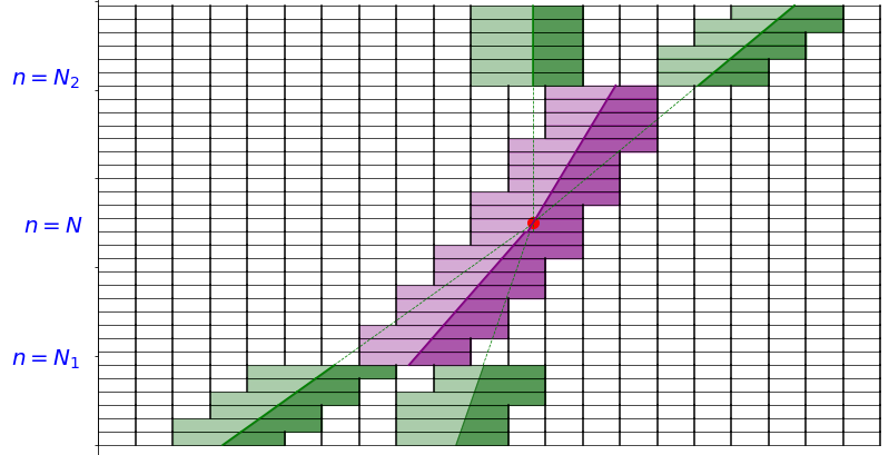
For the sake of clarity, suppose that we only have two trajectories/constraints $(y_{i},q_{i})$ , $i\in\{1,2\}$ , defined on $[0,\tau]$ , which cross at time $\tau$ . We denote by $\mathcal{C}$ this crossing point. Suppose also that this crossing point results in two additional trajectories/constraints $(y_{i},q_{i})$ , $i\in\{3,4\}$ , defined on $[\tau,T]$ , and which do not cross, as represented in Figure 4.

Let us fully make explicit the steps of the reasoning leading to the construction of our scheme in that situation. Suppose that $\lambda=\Delta t/\Delta x$ is fixed and verifies the CFL condition

2\left(\underbrace{\|f^{\prime}\|_{\mathbf{L}^{\infty}}+\max_{i\in[\![1;4]\!]}\|\dot{y}_{i}\|_{\mathbf{L}^{\infty}(\mathopen{]}0,T\mathclose{[})}}_{:=L}\right)\lambda\leq 1.

(4.10)

Set $N\in\mathbb{N}$ such that $\tau\in[t^{N},t^{N+1}\mathclose{[}$ . We divide the discussion in four parts.

Part 1. Introduce the number

N_{1}:=\inf\left\{n\in\mathbb{N}\;:\;|y_{\Delta}^{1}(t^{n})-y_{\Delta}^{2}(t^{n})|\leq 4\Delta x\right\}.

The definition of $N_{1}$ ensures that for all $n\in[\![0;N_{1}-1]\!]$ , we can independently modify the mesh near the two trajectories $y_{\Delta}^{1}$ and $y_{\Delta}^{2}$ , as presented in Figure 5.

Consequently, we can simply define the approximate solution $\rho_{\Delta}$ on $\mathbb{R}\times[0,t^{N_{1}-1}]$ as the finite volume approximation of a conservation law, with initial datum $\rho_{o}$ , with flux constraints on two non-interacting trajectories, using the recipe of Section 3 for each trajectory/constraint.

Part 2. Fix now $n\in[\![N_{1};N]\!]$ . In these time intervals, since the two trajectories are too close to each other, one cannot modify the mesh in the neighborhood of one of them without affecting the other. However, the scheme has to be defined globally, so we proceed as described below.

•

First, introduce the mean trajectory and the new constraint:

$\forall t\in[0,\tau],\quad y_{12}(t):=\frac{y_{1}(t)+y_{2}(t)}{2};\quad q_{12}(t):=\min\{q_{1}(t),q_{2}(t)\},$

represented in purple in Figure 5, before the crossing point (in red). The choice of taking the minimal level of constraint in the definition of $q_{12}$ stems from the nature of the constrained problem; see however Remark 4.1 below.

•

Then, define $\rho_{\Delta}$ on $\mathbb{R}\times[t^{N_{1}},t^{N}]$ as the finite volume approximation of the one trajectory/one constraint problem:

\left\{\begin{aligned} \partial_{t}\rho+\partial_{x}\left(f(\rho)\right)&=0\\ \rho(\cdot,t^{N_{1}})&=\rho_{\Delta}(\cdot,t^{N_{1}-1})\\ \left.\left(f(\rho)-\dot{y}_{12}(t)\rho\right)\right|_{x=y_{12}(t)}&\leq q_{12}(t)&t\in\mathopen{]}t^{N_{1}},t^{N}\mathclose{[},\end{aligned}\right.

using exactly the recipe of Section 3.1.

Part 3. Introduce the number:

N_{2}:=\inf\left\{n\in\mathbb{N}\;:\;n>N\;\;\text{and}\;\;|y_{\Delta}^{3}(t^{n})-y_{\Delta}^{4}(t^{n})|\geq 4\Delta x\right\}.

For $n\in[\![N;N_{2}]\!]$ , we are in the same situation as Part 2. We proceed to the same construction, mutatis mutandis.

•

As in Part 2, define the mean trajectory and the new constraint:

$\forall t\in[\tau,T],\quad y_{34}(t):=\frac{y_{3}(t)+y_{4}(t)}{2};\quad q_{34}(t):=\min\{q_{3}(t),q_{4}(t)\},$

represented in purple in Figure 5, after the crossing point.

•

Define $\rho_{\Delta}$ on $\mathbb{R}\times[t^{N},t^{N_{2}}]$ as the finite volume approximation of the one trajectory/one constraint problem:

\left\{\begin{aligned} \partial_{t}\rho+\partial_{x}\left(f(\rho)\right)&=0\\ \rho(\cdot,t^{N})&=\rho_{\Delta}(\cdot,t^{N})\\ \left.\left(f(\rho)-\dot{y}_{34}(t)\rho\right)\right|_{x=y_{34}(t)}&\leq q_{34}(t)&t\in\mathopen{]}t^{N},t^{N_{2}}\mathclose{[}.\end{aligned}\right.

Part 4. Finally, $\rho_{\Delta}$ is defined on $\mathbb{R}\times[t^{N_{2}},T]$ like in Part 1 with $y_{3},q_{3},\rho_{\Delta}(\cdot,t^{N_{2}})$ (resp. $y_{4},q_{4}$ ) playing the role of $y_{1},q_{1},\rho_{o}$ (resp. of $y_{2},q_{2}$ ).

Remark 4.1.

Let us stress out that the details of the treatment done in Parts 2-3 do not play any significant role in the convergence proof below thanks to the choice of test functions vanishing at neighborhood of the crossing points, see Proposition 4.5. Consequently, taking the mean trajectory and the minimum of the constraint is merely an example aiming at preserving some consistency while keeping the scheme simple to understand and implement.

The general case of a finite number of interfaces (locally finite number can be easily included) is treated in the same way, leading to a pattern with the uniform rectangular mesh adapted to each of the interfaces $\Gamma_{i}$ , $i\in[\![1;J]\!]$ except for small (in terms of the number of impacted mesh cells) neighborhoods of the crossing points $\mathcal{C}_{m}$ , $m\in[\![1;M]\!]$ .

4.3.2 Proof of convergence

Theorem 4.6.

Fix $T>0$ , $f\in\mathbf{C}^{2}([0,1],\mathbb{R}^{+})$ satisfying (1.1)-(3.14) and $\rho_{o}\in\mathbf{L}^{\infty}(\mathbb{R},[0,1])$ . Let $(y_{i},q_{i})_{i\in[\![1;J]\!]}$ be a finite family of trajectories and constraints defined on $\mathopen{]}s_{i},T_{i}\mathclose{[}$ ( $0\leq s_{i}<T_{i}$ ). We suppose that for all $i\in[\![1;J]\!]$ , $y_{i}\in\mathbf{W}^{1,\infty}(\mathopen{]}s_{i},T_{i}\mathclose{[},\mathbb{R})$ and $q_{i}\in\mathbf{L}^{\infty}(\mathopen{]}s_{i},T_{i}\mathclose{[},\mathbb{R}^{+})$ . Suppose also that the interfaces $(\Gamma_{i})_{i}$ defined by the trajectories $(y_{i})_{i}$ have a finite number of crossing points. Then as $\Delta\to 0$ while satisfying the CFL condition

2\left(\underbrace{\|f^{\prime}\|_{\mathbf{L}^{\infty}}+\max_{i\in[\![0;J]\!]}\|\dot{y}_{i}\|_{\mathbf{L}^{\infty}(\mathopen{]}0,T\mathclose{[})}}_{:=L}\right)\lambda\leq 1,

the sequence $(\rho_{\Delta})_{\Delta}$ constructed by the procedure of Section 4.3.1 converges a.e. on $\Omega$ to the admissible entropy solution to (1.2).

Proof. We make use of the fact that in Definition 4.4, we only need to consider test functions that vanish at a neighborhood of the crossing points (this is the key observation leading to Remark 4.1 here above).

(i) Proof of the entropy inequalities. Fix $\varphi\in\mathbf{C}_{\mathbf{c}}^{\infty}(\overline{\Omega}\backslash\cup_{m=1}^{M}\mathcal{C}_{m},\mathbb{R}^{+})$ , written as $\varphi=\varphi_{o}+\sum_{i=1}^{J}\varphi_{i}$ , using the appropriate partition of unity, see Section 4.1. Since $\varphi_{o}$ vanishes along all the interfaces, $\rho_{\Delta}$ verifies inequality (3.11) with $\mathcal{R}\equiv 0$ on the domain $\Omega_{o}$ and with test function $\varphi_{o}$ . Indeed, for a sufficiently small $\Delta x>0$ , the scheme we constructed in the previous section reduces to a standard finite volume in $\Omega_{o}$ . Fix now $i\in[\![1;J]\!]$ . Since $\varphi_{i}$ vanishes along all the interfaces but $\Gamma_{i}$ , $\rho_{\Delta}$ verifies inequality (3.11) with reminder term $\mathcal{R}_{s_{\Delta}^{i}}(\kappa,q_{\Delta}^{i})$ along the trajectory $y_{\Delta}^{i}$ on the domain $\Omega_{i}$ and with test function $\varphi_{i}$ , due to the analysis of Section 3; indeed, in the support of the test function, our scheme for the multi-interface problem reduces to the scheme for the single-interface problem. By summing these previous inequalities, we obtain an approximate version of (4.8) verified by $\rho_{\Delta}$ :

	$\displaystyle\int_{0}^{+\infty}\int_{\mathbb{R}}$	$\displaystyle\biggl{(}\|\rho_{\Delta}-\kappa\|\partial_{t}\varphi+\Phi_{\Delta}(\rho_{\Delta},\kappa)\partial_{x}\varphi\biggr{)}\mathinner{\mathrm{d}{x}}\mathinner{\mathrm{d}{t}}+\int_{\mathbb{R}}\|\rho_{\Delta}^{0}(x)-\kappa\|\varphi(x,0)\mathinner{\mathrm{d}{x}}$		(4.11)
		$\displaystyle+\sum_{i=1}^{J}\int_{s_{i}}^{T_{i}}\mathcal{R}_{s_{\Delta}^{i}(t)}(\kappa,q_{\Delta}^{i}(t))\varphi(y_{\Delta}^{i}(t),t)\mathinner{\mathrm{d}{t}}\geq\mathop{}\mathopen{}O\mathopen{}\left(\Delta x\right)+\mathop{}\mathopen{}O\mathopen{}\left(\Delta t\right).$		(4.11)

(ii) Proof of the weak constraint inequalities. Let $\varphi\in\mathbf{C}_{\mathbf{c}}^{\infty}(\Omega\backslash\cup_{m=1}^{M}\mathcal{C}_{m},\mathbb{R}^{+})$ , written under the form (4.1). Fix $i\in[\![1;J]\!]$ . Since $\varphi_{i}$ vanishes along all the interfaces but $\Gamma_{i}$ , for a sufficiently small $\Delta x$ , $\rho_{\Delta}$ verifies inequality (3.13) with constraint $q_{\Delta}^{i}$ along the trajectory $y_{\Delta}^{i}$ on the domain $\Omega_{i}^{+}$ and with test function $\varphi_{i}$ . We obtain an approximate version of (4.12) verified by $\rho_{\Delta}$ :

-\iint_{\Omega_{i}^{+}}\biggl{(}\rho_{\Delta}\partial_{t}\varphi+\mathbf{F}_{\Delta}(\rho_{\Delta})\partial_{x}\varphi\biggr{)}\mathinner{\mathrm{d}{x}}\mathinner{\mathrm{d}{t}}\leq\int_{s_{i}}^{T_{i}}q_{\Delta}^{i}(t)\varphi_{i}(y_{\Delta}^{i}(t),t)\mathinner{\mathrm{d}{t}}+\mathop{}\mathopen{}O\mathopen{}\left(\Delta x\right)+\mathop{}\mathopen{}O\mathopen{}\left(\Delta t\right).

(4.12)

(iii) Compactness and convergence. Compactness of the sequence $(\rho_{\Delta})_{\Delta}$ follows directly from the study of Section 3.4 where we derived local $\mathbf{BV}$ bounds for $(\rho_{\Delta})_{\Delta}$ under the assumption (3.14). Indeed, these local bounds lead to compactness in the domain complementary to the interfaces, we only use the fact that the interfaces together with the crossing points form a closed subset of $\Omega$ with zero Lebesgue measure. Once the a.e. convergence (up to a subsequence) on $\Omega$ to some $\rho\in\mathbf{L}^{\infty}(\Omega,[0,1])$ obtained, we simply pass to the limit in (4.11)-(4.12). This proves that $\rho$ is an admissible solution to (1.2). By the uniqueness of Theorem 4.3, the whole sequence converges to $\rho$ . This concludes the proof. $\square$

Corollary 4.7.

Fix $T>0$ , $f\in\mathbf{C}^{2}([0,1],\mathbb{R}^{+})$ satisfying (1.1)-(3.14) and $\rho_{o}\in\mathbf{L}^{\infty}(\mathbb{R},[0,1])$ . Let $(y_{i},q_{i})_{i\in[\![1;J]\!]}$ be a finite family of trajectories and constraints defined on $\mathopen{]}s_{i},T_{i}\mathclose{[}$ ( $0\leq s_{i}<T_{i}$ ). We suppose that for all $i\in[\![1;J]\!]$ , $y_{i}\in\mathbf{W}^{1,\infty}(\mathopen{]}s_{i},T_{i}\mathclose{[},\mathbb{R})$ and $q_{i}\in\mathbf{L}^{\infty}(\mathopen{]}s_{i},T_{i}\mathclose{[},\mathbb{R}^{+})$ . Suppose also that the interfaces $(\Gamma_{i})_{i}$ defined by the trajectories $(y_{i})_{i}$ have a finite number of crossing points. Then Problem (1.2) admits a unique admissible entropy solution.

Proof. Existence comes from Theorem 4.6 while uniqueness is established by Theorem 4.3. $\square$

5 Numerical experiment with crossing trajectories

In this section, we perform a numerical test to illustrate the scheme analyzed in Section 3 and Section 4.3. We take the GNL flux $f(\rho)=\rho(1-\rho)$ .

We model the following situation. A vehicle breaks down on a road and reduces by half the surrounding traffic flow, which initial state is given by $\displaystyle{\rho_{o}=0.8\times\mathbf{1}_{[1,3]}}$ . At some point, a tow truck comes to move the immobile vehicle. We summarized this situation in Figure 6. Notice the time interval in which $q_{3}\equiv 0.1$ . This corresponds to the time needed for the tow truck to move the vehicle. Remark also that the value of the constraint on this time interval is smaller than the one when only the broken down vehicle was reducing the traffic flow.

The evolution of the numerical solution is represented in Figure 7. Let us comment on the profile of the numerical solution.

•

At first ( $0\leq t\leq 5.80$ ), the solution is composed of traveling waves separated by a stationary non-classical shock located at the immobile vehicle position.
•

When the tow truck catches up with the vehicle ( $6.30\leq t\leq 8.0$ ), the profile of the numerical solution is the same, but the greater value of the constraint in this time interval changes the magnitude of the non-classical shock; at this point the combined presence of both the tow truck and the immobile vehicle clogs the traffic flow even more.
•

Finally, once the tow truck starts again ( $t>8.0$ ), the traffic congestion is reduced.

Notice at time $t=7.44$ the small artifact (circled in red in Figure 7) created by Parts 2-3 in the construction of the approximate solution and reproduced by the scheme. This highlights the fact that even if the treatment of the crossing points brings inconsistencies or artifacts to the numerical solution, these undesired effects are not amplified by the scheme, and become negligible when one refines the mesh.

Appendix A Proof of the OSL bound

We prove in this appendix Lemma 3.5. All the notations are taken from Sections 3.1 and 3.4. The proof is a simple rewriting of the proof of [22, Lemma 4.2].

It will be convenient to write the Engquist-Osher flux under the form:

\forall a,b\in[0,1],\quad\mathbf{EO}(a,b)=\underbrace{\left(f(a\wedge\overline{\rho})-\frac{f(\overline{\rho})}{2}\right)}_{q_{+}(a)}+\underbrace{\left(f(b\vee\overline{\rho})-\frac{f(\overline{\rho})}{2}\right)}_{q_{-}(b)},

so that for all $n\in\mathbb{N}$ , when $j\in\widehat{\mathbb{Z}}_{n+1}$ , the scheme (3.4) can be rewritten as:

\rho_{j+1/2}^{n+1}=\rho_{j+1/2}^{n}-\lambda\biggl{(}q_{+}\left(\rho_{j+1/2}^{n}\right)+q_{-}\left(\rho_{j+3/2}^{n}\right)-q_{+}\left(\rho_{j-1/2}^{n}\right)-q_{-}\left(\rho_{j+1/2}^{n}\right)\biggr{)}.

(A.1)

Lemma A.1.

For all $n\in\mathbb{N}$ and $j\in\mathbb{Z}$ , we have

\rho_{j-1/2}^{n}-\rho_{j+1/2}^{n}\leq\frac{1}{\lambda\mu}\quad\text{and}\quad D_{j}^{n}\leq\frac{1}{\lambda\mu}.

(A.2)

Proof. Indeed, using first the uniform convexity of $f$ and then the CFL condition (3.2), we can write:

\left(\rho_{j-1/2}^{n}-\rho_{j+1/2}^{n}\right)\mu\leq-\int_{\rho_{j+1/2}^{n}}^{\rho_{j-1/2}^{n}}f^{\prime\prime}(u)\mathinner{\mathrm{d}{u}}\leq 2\|f^{\prime}\|_{\mathbf{L}^{\infty}}\leq\frac{\Delta x}{\Delta t},

from which we deduce (A.2). $\square$

Lemma A.2.

Let $n\in\mathbb{N}$ , $j\in\widehat{\mathbb{Z}}_{n+1}$ , $\displaystyle{a=\frac{\lambda\mu}{4}}$ and $\displaystyle{\psi(x)=x-ax^{2}}$ . Then

D_{j}^{n+1}\leq\psi\left(\max\left\{D_{j-1}^{n},D_{j}^{n},D_{j+1}^{n}\right\}\right).

(A.3)

Proof. We divide the proof in three steps.

Step 1: The function $\psi$ is nonnegative on $[0,1/a]$ and nondecreasing on $[0,1/(2a)]$ . Note that by (A.2), $\displaystyle{\max\left\{D_{j-1}^{n},D_{j}^{n},D_{j+1}^{n}\right\}\leq 1/(4a)}$ , which will allow us to use the monotonicity of $\psi$ .

Step 2. We assume that

\rho_{j+1/2}^{n}-\rho_{j+3/2}^{n}\geq 0\quad\text{and}\quad\rho_{j-3/2}^{n}-\rho_{j-1/2}^{n}\geq 0,

(A.4)

and we are going to prove that (A.3) holds. Using the uniform concavity assumption of $f$ , we can write that

\forall a,b\in[0,1],\quad q_{+}(b)-q_{+}(a)\leq(b\wedge\overline{\rho}-a\wedge\overline{\rho})f^{\prime}(a\wedge\overline{\rho})-\frac{\mu}{2}(b\wedge\overline{\rho}-a\wedge\overline{\rho})^{2}.

(A.5)

A similar inequality holds for $q_{-}$ as well. Using (A.1), we obtain:

$\displaystyle\rho_{j-1/2}^{n+1}-\rho_{j+1/2}^{n+1}$	$\displaystyle=\rho_{j-1/2}^{n}-\rho_{j+1/2}^{n}$	(A.6)
	$\displaystyle-\lambda\left(q_{+}\left(\rho_{j-1/2}^{n}\right)-q_{+}\left(\rho_{j-3/2}^{n}\right)-q_{+}\left(\rho_{j+1/2}^{n}\right)+q_{+}\left(\rho_{j-1/2}^{n}\right)\right)$
	$\displaystyle-\lambda\left(q_{-}\left(\rho_{j+1/2}^{n}\right)-q_{-}\left(\rho_{j-1/2}^{n}\right)-q_{-}\left(\rho_{j+3/2}^{n}\right)+q_{-}\left(\rho_{j+1/2}^{n}\right)\right)$
	$\displaystyle=\rho_{j-1/2}^{n}-\rho_{j+1/2}^{n}$
	$\displaystyle+\lambda\left\{\left(q_{+}\left(\rho_{j+1/2}^{n}\right)-q_{+}\left(\rho_{j-1/2}^{n}\right)\right)+\left(q_{+}\left(\rho_{j-3/2}^{n}\right)-q_{+}\left(\rho_{j-1/2}^{n}\right)\right)\right.$
	$\displaystyle\left.+\left(q_{-}\left(\rho_{j+3/2}^{n}\right)-q_{-}\left(\rho_{j+1/2}^{n}\right)\right)+\left(q_{-}\left(\rho_{j-1/2}^{n}\right)-q_{-}\left(\rho_{j+1/2}^{n}\right)\right)\right\}$
	$\displaystyle\leq\rho_{j-1/2}^{n}-\rho_{j+1/2}^{n}$
	$\displaystyle+\lambda\left(\rho_{j+1/2}^{n}\wedge\overline{\rho}-\rho_{j-1/2}^{n}\wedge\overline{\rho}\right)f^{\prime}(\rho_{j-1/2}^{n}\wedge\overline{\rho})-\frac{\lambda\mu}{2}\left(\rho_{j+1/2}^{n}\wedge\overline{\rho}-\rho_{j-1/2}^{n}\wedge\overline{\rho}\right)^{2}$
	$\displaystyle+\lambda\left(\rho_{j-3/2}^{n}\wedge\overline{\rho}-\rho_{j-1/2}^{n}\wedge\overline{\rho}\right)f^{\prime}(\rho_{j-1/2}^{n}\wedge\overline{\rho})-\frac{\lambda\mu}{2}\left(\rho_{j-3/2}^{n}\wedge\overline{\rho}-\rho_{j-1/2}^{n}\wedge\overline{\rho}\right)^{2}$
	$\displaystyle+\lambda\left(\rho_{j+3/2}^{n}\vee\overline{\rho}-\rho_{j+1/2}^{n}\vee\overline{\rho}\right)f^{\prime}(\rho_{j+1/2}^{n}\vee\overline{\rho})-\frac{\lambda\mu}{2}\left(\rho_{j+3/2}^{n}\vee\overline{\rho}-\rho_{j+1/2}^{n}\vee\overline{\rho}\right)^{2}$
	$\displaystyle+\lambda\left(\rho_{j-1/2}^{n}\vee\overline{\rho}-\rho_{j+1/2}^{n}\vee\overline{\rho}\right)f^{\prime}(\rho_{j+1/2}^{n}\vee\overline{\rho})-\frac{\lambda\mu}{2}\left(\rho_{j-1/2}^{n}\vee\overline{\rho}-\rho_{j+1/2}^{n}\vee\overline{\rho}\right)^{2},$

where the last inequality comes from using (A.5). The proof now reduces to four cases, depending on the ordering of $\overline{\rho}$ , $\rho_{j-1/2}^{n}$ and $\rho_{j-1/2}^{n}$ .

Case 1: $\overline{\rho}\geq\rho_{j-1/2}^{n},\ \rho_{j+1/2}^{n}$ . Under assumption (A.4), we have $\overline{\rho}\geq\rho_{j+3/2}^{n}$ as well. Inequality (A.6) becomes:

$\displaystyle\rho_{j-1/2}^{n+1}-\rho_{j+1/2}^{n+1}$	$\displaystyle\leq\left(1-\lambda f^{\prime}(\rho_{j-1/2}^{n})\right)\left(\rho_{j-1/2}^{n}-\rho_{j+1/2}^{n}\right)+\lambda f^{\prime}(\rho_{j-1/2}^{n})\left(\rho_{j-3/2}^{n}\wedge\overline{\rho}-\rho_{j-1/2}^{n}\right)$	(A.7)
	$\displaystyle-\frac{\lambda\mu}{2}\left(\left(\rho_{j-1/2}^{n}-\rho_{j+1/2}^{n}\right)^{2}+\left(\rho_{j-3/2}^{n}\wedge\overline{\rho}-\rho_{j-1/2}^{n}\right)^{2}\right)$
	$\displaystyle\leq\left(1-\lambda f^{\prime}(\rho_{j-1/2}^{n})\right)\left(\rho_{j-1/2}^{n}-\rho_{j+1/2}^{n}\right)+\lambda f^{\prime}(\rho_{j-1/2}^{n})\left(\rho_{j-3/2}^{n}\wedge\overline{\rho}-\rho_{j-1/2}^{n}\right)$
	$\displaystyle-\frac{\lambda\mu}{4}\left(\left(\rho_{j-1/2}^{n}-\rho_{j+1/2}^{n}\right)^{2}+\left(\rho_{j-3/2}^{n}\wedge\overline{\rho}-\rho_{j-1/2}^{n}\right)^{2}\right)$
	$\displaystyle\leq\left(1-\lambda f^{\prime}(\rho_{j-1/2}^{n})\right)\left(\rho_{j-1/2}^{n}-\rho_{j+1/2}^{n}\right)+\lambda f^{\prime}(\rho_{j-1/2}^{n}\left(\rho_{j-3/2}^{n}\wedge\overline{\rho}-\rho_{j-1/2}^{n}\right)$
	$\displaystyle-\frac{\lambda\mu}{4}\max\left\{\rho_{j-1/2}^{n}-\rho_{j+1/2}^{n},\rho_{j-3/2}^{n}\wedge\overline{\rho}-\rho_{j-1/2}^{n}\right\}^{2},$

where the last inequality comes from the bound: $\displaystyle{a^{2}+b^{2}\geq\max\{a,b\}^{2}}$ . The CFL condition (3.2) ensures that the two first terms of the right-hand side of the last inequality are a convex combination of $\displaystyle{\left(\rho_{j-1/2}^{n}-\rho_{j+1/2}^{n}\right)}$ and $\displaystyle{\left(\rho_{j-3/2}^{n}\wedge\overline{\rho}-\rho_{j-1/2}^{n}\right)}$ . Consequently, inequality (A.7) then becomes

\rho_{j-1/2}^{n+1}-\rho_{j+1/2}^{n+1}\leq\psi\left(\max\left\{\rho_{j-1/2}^{n}-\rho_{j+1/2}^{n},\rho_{j-3/2}^{n}\wedge\overline{\rho}-\rho_{j-1/2}^{n}\right\}\right).

Since $\displaystyle{\rho_{j-3/2}^{n}\wedge\overline{\rho}-\rho_{j-1/2}^{n}\leq\rho_{j-3/2}^{n}-\rho_{j-1/2}^{n}}$ , the monotonicity of $\psi$ ensures that

	$\displaystyle\rho_{j-1/2}^{n+1}-\rho_{j+1/2}^{n+1}$	$\displaystyle\leq\psi\left(\max\left\{\rho_{j-1/2}^{n}-\rho_{j+1/2}^{n},\rho_{j-3/2}^{n}-\rho_{j-1/2}^{n}\right\}\right)$
		$\displaystyle\leq\psi\left(\max\left\{D_{j-1}^{n},D_{j}^{n}\right\}\right)$
		$\displaystyle\leq\psi\left(\max\left\{D_{j-1}^{n},D_{j}^{n},D_{j+1}^{n}\right\}\right).$

Since the right-hand side of this inequality is nonnegative, we can replace its left-hand side by $D_{j}^{n+1}$ , which concludes the proof in this case.

Case 2: $\overline{\rho}\leq\rho_{j-1/2}^{n},\ \rho_{j+1/2}^{n}$ . The proof of in this case similar to the last one so we omit the details.

Case 3: $\rho_{j+1/2}^{n}\leq\overline{\rho}\leq\rho_{j-1/2}^{n}$ . Under Assumption (A.4), we have the following ordering:

\rho_{j+3/2}^{n}\leq\rho_{j+1/2}^{n}\leq\overline{\rho}\leq\rho_{j-1/2}^{n}\leq\rho_{j-3/2}^{n}.

Inequality (A.6) becomes

	$\displaystyle\rho_{j-1/2}^{n+1}-\rho_{j+1/2}^{n+1}$	$\displaystyle\leq\rho_{j-1/2}^{n}-\rho_{j+1/2}^{n}-\frac{\lambda\mu}{2}\left((\rho_{j-1/2}^{n}-\overline{\rho})^{2}+(\overline{\rho}-\rho_{j+1/2}^{n})^{2}\right)$
		$\displaystyle\leq\rho_{j-1/2}^{n}-\rho_{j+1/2}^{n}-\frac{\lambda\mu}{4}(\rho_{j-1/2}^{n}-\rho_{j+1/2}^{n})^{2},$

where we used the inequality $2(a^{2}+b^{2})\geq(a+b)^{2}$ . From here, we can conclude as in Case 1.

Case 4: $\rho_{j-1/2}^{n}\leq\overline{\rho}\leq\rho_{j+1/2}^{n}$ . Using the decomposition

\rho_{j-1/2}^{n}-\rho_{j+1/2}^{n}=(\rho_{j-1/2}^{n}\wedge\overline{\rho}-\rho_{j+1/2}^{n}\wedge\overline{\rho})+(\rho_{j-1/2}^{n}\vee\overline{\rho}-\rho_{j+1/2}^{n}\vee\overline{\rho}),

inequality (A.6) becomes

$\displaystyle\rho_{j-1/2}^{n+1}-\rho_{j+1/2}^{n+1}$	$\displaystyle\leq\left(1-\lambda f^{\prime}(\rho_{j-1/2}^{n})\right)\left(\rho_{j-1/2}^{n}\wedge\overline{\rho}-\rho_{j+1/2}^{n}\wedge\overline{\rho}\right)+\lambda f^{\prime}(\rho_{j-1/2}^{n})\left(\rho_{j-3/2}^{n}\wedge\overline{\rho}-\rho_{j-1/2}^{n}\wedge\overline{\rho}\right)$	(A.8)
	$\displaystyle+\left(1+\lambda f^{\prime}(\rho_{j+1/2}^{n})\right)\left(\rho_{j-1/2}^{n}\vee\overline{\rho}-\rho_{j+1/2}^{n}\vee\overline{\rho}\right)-\lambda f^{\prime}(\rho_{j+1/2}^{n})\left(\rho_{j+1/2}^{n}\vee\overline{\rho}-\rho_{j+3/2}^{n}\vee\overline{\rho}\right)$
	$\displaystyle-\frac{\lambda\mu}{2}\left\{\left(\rho_{j-1/2}^{n}\wedge\overline{\rho}-\rho_{j+1/2}^{n}\wedge\overline{\rho}\right)^{2}+\left(\rho_{j-3/2}^{n}\wedge\overline{\rho}-\rho_{j-1/2}^{n}\wedge\overline{\rho}\right)^{2}\right.$
	$\displaystyle\left.+\left(\rho_{j-1/2}^{n}\vee\overline{\rho}-\rho_{j+1/2}^{n}\vee\overline{\rho}\right)^{2}+\left(\rho_{j+1/2}^{n}\vee\overline{\rho}-\rho_{j+3/2}^{n}\vee\overline{\rho}\right)^{2}\right\}$
	$\displaystyle\leq\left(1-\lambda f^{\prime}(\rho_{j-1/2}^{n})\right)\left(\rho_{j-1/2}^{n}\wedge\overline{\rho}-\rho_{j+1/2}^{n}\wedge\overline{\rho}\right)+\lambda f^{\prime}(\rho_{j-1/2}^{n})\left(\rho_{j-3/2}^{n}\wedge\overline{\rho}-\rho_{j-1/2}^{n}\wedge\overline{\rho}\right)$
	$\displaystyle+\left(1+\lambda f^{\prime}(\rho_{j+1/2}^{n})\right)\left(\rho_{j-1/2}^{n}\vee\overline{\rho}-\rho_{j+1/2}^{n}\vee\overline{\rho}\right)-\lambda f^{\prime}(\rho_{j+1/2}^{n})\left(\rho_{j+1/2}^{n}\vee\overline{\rho}-\rho_{j+3/2}^{n}\vee\overline{\rho}\right)$
	$\displaystyle-\frac{\lambda\mu}{2}\left\{\left(\rho_{j-1/2}^{n}\wedge\overline{\rho}-\rho_{j+1/2}^{n}\wedge\overline{\rho}\right)^{2}+\left(\rho_{j-1/2}^{n}\vee\overline{\rho}-\rho_{j+1/2}^{n}\vee\overline{\rho}\right)^{2}\right\}.$

The CFL condition (3.2) and the ordering $\rho_{j+1/2}^{n}\leq\overline{\rho}\leq\rho_{j-1/2}^{n}$ result in

\left(1-\lambda f^{\prime}(\rho_{j-1/2}^{n})\right)\left(\rho_{j-1/2}^{n}\wedge\overline{\rho}-\rho_{j+1/2}^{n}\wedge\overline{\rho}\right)\leq 0\quad\text{and}\quad\left(1+\lambda f^{\prime}(\rho_{j+1/2}^{n})\right)\left(\rho_{j-1/2}^{n}\vee\overline{\rho}-\rho_{j+1/2}^{n}\vee\overline{\rho}\right)\leq 0

so we can replace (A.8) by

	$\displaystyle\rho_{j-1/2}^{n+1}-\rho_{j+1/2}^{n+1}$	$\displaystyle\leq\lambda f^{\prime}(\rho_{j-1/2}^{n})\left(\rho_{j-3/2}^{n}\wedge\overline{\rho}-\rho_{j-1/2}^{n}\wedge\overline{\rho}\right)-\lambda f^{\prime}(\rho_{j+1/2}^{n})\left(\rho_{j+1/2}^{n}\vee\overline{\rho}-\rho_{j+3/2}^{n}\vee\overline{\rho}\right)$
		$\displaystyle-\frac{\lambda\mu}{2}\left\{\left(\rho_{j-1/2}^{n}\wedge\overline{\rho}-\rho_{j+1/2}^{n}\wedge\overline{\rho}\right)^{2}+\left(\rho_{j-1/2}^{n}\vee\overline{\rho}-\rho_{j+1/2}^{n}\vee\overline{\rho}\right)^{2}\right\}$
		$\displaystyle\leq\frac{1}{2}\left(\left(\rho_{j-3/2}^{n}\wedge\overline{\rho}-\rho_{j-1/2}^{n}\wedge\overline{\rho}\right)+\left(\rho_{j+1/2}^{n}\vee\overline{\rho}-\rho_{j+3/2}^{n}\vee\overline{\rho}\right)\right)$
		$\displaystyle-\frac{\lambda\mu}{4}\left\{\left(\rho_{j-1/2}^{n}\wedge\overline{\rho}-\rho_{j+1/2}^{n}\wedge\overline{\rho}\right)^{2}+\left(\rho_{j-1/2}^{n}\vee\overline{\rho}-\rho_{j+1/2}^{n}\vee\overline{\rho}\right)^{2}\right\}$
		$\displaystyle\leq\psi\left(\max\left\{\left(\rho_{j-3/2}^{n}\wedge\overline{\rho}-\rho_{j-1/2}^{n}\wedge\overline{\rho}\right),\left(\rho_{j-1/2}^{n}\vee\overline{\rho}-\rho_{j+1/2}^{n}\vee\overline{\rho}\right)\right\}\right),$

and we exploit the monotonicity of $\psi$ to conclude.

Step 3: We no longer assume (A.4), and we get back to the general case. Let us introduce

u_{j-3/2}^{n}=\rho_{j-3/2}^{n}\vee\rho_{j-1/2}^{n},\;u_{j-1/2}^{n}=\rho_{j-1/2}^{n},\;u_{j+1/2}^{n}=\rho_{j+1/2}^{n},\;u_{j+3/2}^{n}=\rho_{j+3/2}^{n}\wedge\rho_{j-1/2}^{n},

and

u_{j-1/2}^{n+1}=H(u_{j-3/2}^{n},u_{j-1/2}^{n},u_{j+1/2}^{n});\quad u_{j+1/2}^{n+1}=H(u_{j-1/2}^{n},u_{j+1/2}^{n},u_{j+3/2}^{n}).

Using the monotonicity of $H$ , we get:

	$\displaystyle\rho_{j-1/2}^{n+1}-\rho_{j+1/2}^{n+1}$	$\displaystyle=H(\rho_{j-3/2}^{n},\rho_{j-1/2}^{n},\rho_{j+1/2}^{n})-H(\rho_{j-1/2}^{n},\rho_{j+1/2}^{n},\rho_{j+3/2}^{n})$
		$\displaystyle\leq H(u_{j-3/2}^{n},u_{j-1/2}^{n},u_{j+1/2}^{n})-H(u_{j-1/2}^{n},u_{j+1/2}^{n},u_{j+3/2}^{n})=u_{j-1/2}^{n+1}-u_{j+1/2}^{n+1}.$

Since $u_{j+1/2}^{n}-u_{j+3/2}^{n}\geq 0$ and $u_{j-3/2}^{n}-u_{j-1/2}^{n}\geq 0$ , Step 2 ensures that

{\overset{\sim}{D}}_{j}^{n+1}\leq\psi\left(\max\left\{{\overset{\sim}{D}}_{j-1}^{n},{\overset{\sim}{D}}_{j}^{n},{\overset{\sim}{D}}_{j+1}^{n}\right\}\right),\quad{\overset{\sim}{D}}_{j}^{n}=\max\left\{u_{j-1/2}^{n}-u_{j+1/2}^{n},0\right\}.

Clearly,

{\overset{\sim}{D}}_{j-1}^{n}\leq D_{j-1}^{n},\quad{\overset{\sim}{D}}_{j}^{n}=D_{j}^{n},\quad{\overset{\sim}{D}}_{j+1}^{n}\leq D_{j+1}^{n}.

Using the monotonicity of $\psi$ , we get:

\rho_{j-1/2}^{n+1}-\rho_{j+1/2}^{n+1}\leq u_{j-1/2}^{n+1}-u_{j+1/2}^{n+1}\leq\psi\left(\max\left\{D_{j-1}^{n},D_{j}^{n},D_{j+1}^{n}\right\}\right),

References

- [1] B. Andreianov. New approaches to describing admissibility of solutions of scalar conservation laws with discontinuous flux. ESAIM: Proceedings and Surveys, 50:40–65, 2015.
- [2] B. Andreianov, P. Goatin, and N. Seguin. Finite volume schemes for locally constrained conservation laws. Numerische Mathematik, 115(4):609–645, 2010.
- [3] B. Andreianov, K. Karlsen, and N. H. Risebro. A theory of -dissipative solvers for scalar conservation laws with discontinuous flux. Archive for Rational Mechanics and Analysis, 201(1):27–86, 2011.
- [4] B. Andreianov and D. Mitrović. Entropy conditions for scalar conservation laws with discontinuous flux revisited. Ann. Inst. H. Poincaré Anal. Non Linéaire, 32(6):1307–1335, 2015.
- [5] B. Andreianov and A. Sylla. A macroscopic model to reproduce self-organization at bottlenecks. In International Conference on Finite Volumes for Complex Applications, pages 243–254. Springer, 2020.
- [6] A. Bressan, G. Guerra, and W. Shen. Vanishing viscosity solutions for conservation laws with regulated flux. Journal of Differential Equations, 266(1):312–351, 2019.
- [7] C. Chalons, M. L. Delle Monache, and P. Goatin. A conservative scheme for non-classical solutions to a strongly coupled pde-ode problem. Interfaces and Free Boundaries, 19(4):553–570, 2018.
- [8] R. M. Colombo and P. Goatin. A well posed conservation law with a variable unilateral constraint. Journal of Differential Equations, 234(2):654–675, 2007.
- [9] M. L. Delle Monache and P. Goatin. Scalar conservation laws with moving constraints arising in traffic flow modeling: an existence result. Journal of Differential Equations, 257(11):4015––4029, 2014.
- [10] M. L. Delle Monache and P. Goatin. A numerical scheme for moving bottlenecks in traffic flow. Bulletin of the Brazilian Mathematical Society, New Series, 47(2):605–617, 2016.
- [11] M. L. Delle Monache and P. Goatin. Stability estimates for scalar conservation laws with moving flux constraints. Networks and Heterogeneous Media, 12(2):245–258, 2017.
- [12] M. L. Delle Monache, T. Liard, B. Piccoli, R. Stern, and D. Work. Traffic reconstruction using autonomous vehicles. SIAM Journal on Applied Mathematics, 79(5):1748–1767, 2019.
- [13] R. Eymard, T. Gallouët, and R. Herbin. Finite Volume Methods, volume VII of Handbook of Numerical Analysis. North-Holland, Amsterdam, 2000.
- [14] A. Ferrara, P. Goatin, and G. Piacentini. A macroscopic model for platooning in highway traffic. SIAM Journal on Applied Mathematics, 80(1):639–656, 2020.
- [15] M. Garavello, P. Goatin, T. Liard, and B. Piccoli. A multiscale model for traffic regulation via autonomous vehicles. Journal of Differential Equations, 269(7):6088–6124, 2020.
- [16] I. Gasser, C. Lattanzio, and A. Maurizi. Vehicular traffic flow dynamics on a bus route. Multiscale Modeling & Simulation, 11(3):925–942, 2013.
- [17] H. Holden and N. H. Risebro. Front Tracking for Hyperbolic Conservation Laws, volume 152 of Applied Mathematical Sciences. Springer-Verlag New York, 2002.
- [18] K. H. Karlsen and J. D. Towers. Convergence of the lax-friedrichs scheme and stability for conservation laws with a discontinuous space-time dependent flux. Chinese Annals of Mathematics, 25(03):287–318, 2004.
- [19] S. N. Kruzhkov. First order quasilinear equations with several independent variables. Mathematics of the USSR-Sbornik, 81(123):228–255, 1970.
- [20] N. Laurent-Brouty, G. Costeseque, and P. Goatin. A macroscopic traffic flow model accounting for bounded acceleration. SIAM Journal on Applied Mathematics, 81(1):173–189, 2021.
- [21] A. Sylla. Influence of a slow moving vehicle on traffic: Well-posedness and approximation for a mildly nonlocal model. Networks & Heterogeneous Media, 16(2):221–256, 2021.
- [22] J. D. Towers. Convergence via OSLC of the Godunov scheme for a scalar conservation law with time and space flux discontinuities. Numerische Mathematik, 139(4):939–969, 2018.
- [23] J. D. Towers. An existence result for conservation laws having BV spatial flux heterogeneities-without concavity. Journal of Differential Equations, 269(7):5754–5764, 2020.
- [24] A. I. Vol’pert. The spaces BV and quasilinear equations. Matematicheskii Sbornik, 115(2):255–302, 1967.