A Lagrangian Dual-based Theory-guided Deep Neural Network

We first introduce the following mathematical descriptions of governing equations of the underlying physical problem:

where $\Omega\subset R^{d}$ and $t\in\left({0,T}\right)$ denote the spatial and temporal domain, respectively, with $\partial\Omega$ as the spatial boundaries; $L_{p}$ and $L_{p}u$ represent a differential operator and its spatial derivatives, respectively, of $u$; $l$ is a forcing term; and $I$ and $B$ are two other operators which define the initial and boundary conditions, respectively.

As discussed in Eq.1, TgNN incorporates theory into DNN by the summation of corresponding terms. It is constructed based on the following six general parts shown in Eq.6:

where $f:=L_{p}N_{u}\left({x,t}\right)-l\left({x,t,y}\right)$ needs to approach to 0, representing the residual of the partial differential Eq.3; $\left\{{t_{f}^{i},x_{f}^{i},y_{f}^{i}}\right\}_{i=1}^{n_{f}}$ denotes the collocation points of the residual function with the size of $n_{f}$, which can be randomly chosen because no labels are needed for these points; $N_{u}$ is the approximation of a solution $u$ obtained by the (deep) neural network; $n_{d}$ represents the numbers of training data; $n_{IC}$ and $n_{BC}$ denote the collocation points for the evaluation of initial and boundary conditions, respectively; and $n_{EC}$ and $n_{EK}$ denote the collocation points of engineering control and knowledge, respectively.

Having realized the mathematical description of each term, we then convert the original loss function of the TgNN model, which incorporates scientific knowledge and engineering controls, to be re-written as Eq.7:

Following this, a Lagrangian duality framework [20], which incorporates a Lagrangian dual approach into the learning task, is employed to learn this constrained optimization problem and approximate minimizer $L\left(\theta\right)$. Given three multipliers, $\lambda_{1}$, $\lambda_{2}$, and $\lambda_{3}$, corresponding to per constraint, consider the Lagrangian loss function

where $\nu$ can be written as:

According to [20], the previous Lagrangian loss function with respect to multipliers $\lambda_{i}\left({i=1,...,3}\right)$, can then be transformed into a function with the purpose of finding the $\omega$, which can minimize the Lagrangian loss function, solving the optimization problem shown as follows:

Herein, we denote an approximation of the approximated optimizer ${\rm O}$ as $\tilde{\rm O}_{\lambda}={\rm M}\left[{\omega^{*}\left(\lambda\right)}\right]\left({\lambda=\left\{{\lambda_{i}\left|{i=1,...,3}\right.}\right\}}\right)$, which can be produced by an optimizer (in our paper, we use Adam) during the training process.

Next, the above problem is transformed by the Lagrangian dual approach into searching the required optimal multipliers for a max-min problem shown as follows:

The same as [20], we denote this approximation as $\tilde{\rm O}_{\lambda}={\rm M}\left[{\omega^{*}\left({\lambda^{*}}\right)}\right]$.

To summarize [20], the repeated calculation and search process by the Lagrangian dual framework adhere to the following steps:
(a) Learn $\tilde{\rm O}^{k}_{\lambda}$;
(b) Let $y_{j}^{k}=\tilde{\rm O}_{\lambda}\left({d_{j}}\right)$, where $y_{j}^{k}$ denotes the $j$-th training sample, and $d_{j}$ refers to the label;
(c) $\lambda_{i}^{k+1}=\lambda_{i}^{k}+s_{k}\sum\nolimits_{j=1}^{n}{v\left({g\left({y_{j}^{k},d_{j}}\right)\leq 0}\right)},{\rm{}}i=1,...,3$.
where $s_{k}$ and $k$ refer to the update step size and the current iteration, respectively. In our problem, we recommend $s_{k}\in\left[{1.1,1.4}\right]$, and we utilize $s_{k}{\rm{=}}1.25$ in our experiment.

The governing equation of the subsurface flow problem in our experiment can be written as Eq.12:

where $h$ is the hydraulic head that needs to be predicted; and $S_{s}=0.0001$ and $K$ are the specific storage and the hydraulic conductivity field, respectively. When $h$ is approximate with the neural network, ${N_{h}\left({t,x,y;\theta}\right)}$, the residual of the governing equation of flow can be written as:

In Eq.13, the partial derivatives of ${\partial N_{h}\left({t,x,y;\theta}\right)}$ can be calculated in the network while the partial derivatives of ${K\left({x,y}\right)}$ are, in general, required to be computed by numerical difference. Herein, we view the hydraulic conductivity field as a heterogeneous parameter field, i.e., a random field following a specific distribution with corresponding covariance [9]. Since its covariance is known, the Karhunen-Loeve expansion (KLE) is utilized to parameterize this kind of heterogeneous model. As a result, the residual of the governing equation can be re-written as Eq.14:

where ${\bar{Z}\left({x,y}\right)+\sum\limits_{i=1}^{n}{\sqrt{\lambda_{i}}f_{i}\left({x,y}\right)\xi_{i}\left(\tau\right)}}$ represents the hydraulic conductivity field $Z\left({x,y}\right)=\ln K\left({x,\tau}\right)$ with ${\xi_{i}\left(\tau\right)}$ as the $i$-th independent random variable of the field $Z\left({x,y}\right)$. For the sake of fairness, the settings of our experiments remain the same as those in [9], listed in Tab.LABEL:tab:settings. MODFLOW software is adopted to perform the simulations to obtain the required training dataset.

Wang et al. determined a set of $\lambda$ values for TgNN via an ad-hoc procedure, which is $\lambda=\left[{\lambda_{DATA},\lambda_{IC},\lambda_{BC},\lambda_{PDE},\lambda_{EC},\lambda_{EK}}\right]=[1,1,1,100,1,1]$ [9], for this particular problem. To investigate whether there are improvements in predictive accuracy, we utilize this weight setting as one of the compared methods and denote this case as TgNN. In addition, for comparison, we also take a naive approach by setting the weights equally as $\lambda=[1,1,1,1,1,1]$ and denote this case as TgNN-1.

We first compare the above three methods with the number of iterations of 2000. Tab.LABEL:tab:table2 provides the results of error L2 and R2, as well as the training time, with the best result per measure metric being marked in bold.

As shown in Tab.LABEL:tab:table2, TgNN-LD can obtain the best error L2 and R2 results, which are obviously smaller and larger than the other two, respectively. It is worth noting that its training time seems lightly inferior among all three methods, probably due to the extra computation brought by the introduction of three Lagrangian multipliers. However, in comparison with TgNN-1 without any human adjustment, our proposed TgNN-LD achieves much better error L2 and R2 results. Moreover, compared to TgNN, in which the weights are adjusted by expertise, our method can not only save babysitting time in the preliminary stage of determining a better set of weights, but produce superior results, as well.

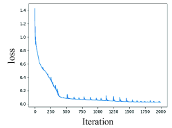
In order to observe the changing trend of each loss, we plot the loss values versus iterations for each method, as shown in Fig.2. Since TgNN places more emphasis on the PDE term, herein, we only provide changes of the total loss (denoted as $loss$), the data term (denoted as $f1\_loss$), and the PDE term (denoted as $f2\_loss$).

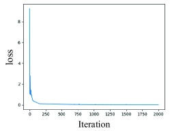
It can be seen from Fig.2 that TgNN-LD can obtain losses with less fluctuation, and TgNN takes second place, and TgNN-1 achieves the worst results. The most remarkable difference lies in changes of $f2\_loss$, which corresponds to the PDE term. The proposed TgNN-LD exhibits much more stable states whereas there are many shocks in both TgNN and TgNN-1. Indeed, in terms of both smoothness and the number of iterations, TgNN-LD achieves superior performance.

Fig.3 compares the correlation between the reference and predicted hydraulic head with the iteration number of 2000. Fig.4 provides prediction results of TgNN-LD, TgNN, and TgNN-1. From these figures, it can be clearly seen that the prediction of TgNN-LD matches the reference values well and are superior to the predictions of the other two.

From Figs.2.(j)-(l), it can be observed that when the number of iterations is approximately 1750, three losses are approaching to converge, suggesting that the number of iterations could be reduced to shorten the training time. To verify its effect, we set different numbers of iterations to test our method. The related results are presented in Tab.III.

As shown in Tab.III, when the number of iteration is 1750, even though the training time is 15s longer than that obtained with the iteration number of 1500, the error L2 and R2 results exhibit the best performance among the compared sets. Especially, in comparison with a result iteration number of 2000, the training time almost decreases by 20%, while the error L2 and R2 results are superior.

To further investigate the effect of Lagrangian multipliers under different iteration values, we plot their changes with iterations, as shown in Fig.5, where Lambda, Lambda1, and Lambda2 refer to $\lambda_{PDE}$, $\lambda_{EC}$, and $\lambda_{EK}$, respectively.

It can be seen from Fig.5 that these Lagrangian multipliers cannot converge to a fixed value, irrespective of the number of iterations, which is rooted in randomly selected seeds leading to various initial values. Tab.IV lists their final values with respect to different settings of iterations.

We then take one set of multipliers (8.1127E+00, 2.8652E-01, and 1.0940E+00) into Eq.1 and keep them the same during the whole training stage to further verify the above conclusion. Related results are shown in Fig.6. From Fig.6, it can be seen that the predictive results obtained by fixed multipliers’ values are not as good as the ones obtained by dynamic changing multipliers.

To investigate the robustness of our proposed method, we add noise with the following formulation into the training data [9]

where $h_{diff}\left({x,y}\right)$, $\alpha\%$, and $\varepsilon$ denote the maximal difference obtained at location $\left({x,y}\right)$ during the entire monitoring process, the noise level, and a uniform variable ranging from -1 to 1.

Figs.7-9 show the predictive results obtained by TgNN-LD, TgNN, and TgNN-1 under noise levels of 5%, 10%, and 20%, respectively, with their error L2 and R2 results listed in Tab.V. From Figs.7-9 and Tab.V, it can be found that TgNN-LD can always obtain the best results among the three methods on correlation between the reference and predicted hydraulic head when noise exists. Moreover, it can also achieve the best results on the error L2 and R2 results. Although the training time obtained by TgNN-LD under different noise levels seems slightly longer than the other two, comparisons between the prediction and reference demonstrate the improvement of incorporating the Lagrangian dual approach.

To investigate the predictive performance more deeply, we substitute the stopping criterion, i.e., a fixed number of iterations, with a dynamic epoch, which has a close relationship with changes of loss values. From Fig.2, it can be seen that the training process has usually already converged with the iteration number of 2000. Therefore, we set the total number of epoch, denoted as $n_{total}$, as 2000. The dynamic epoch is denoted as $n_{D}$.

In our experiment, we maintain a time window with the length of $L_{C}$. For per obtained loss value, we compare whether loss values in the current time window are less than a threshold, $\beta$. If this criterion is satisfied, we stop the iteration and output the predictive results. Herein, we recommend $L_{C}=10$ and $\beta=0.006$. Tab.VI lists a number of good prediction results under the dynamic epoch obtained by TgNN-LD, with their results on correlation between reference and prediction and prediction versus reference being presented in Fig.10. From the numerical results in Tab.VI, it seems that TgNN-LD can come to convergence by a dynamic stopping epoch.

References

- [1] D. Silver, A. Huang, C. J. Maddison, A. Guez, L. Sifre, G. van den Driessche, J. Schrittwieser, I. Antonoglou, V. Panneershelvam, M. Lanctot, S. Dieleman, D. Grewe, J. Nham, N. Kalchbrenner, I. Sutskever, T. Lillicrap, M. Leach, K. Kavukcuoglu, T. Graepel, and D. Hassabis, “Mastering the game of Go with deep neural networks and tree search,” Nature, vol. 529, no. 7587, pp. 484–489, JAN 2016.
- [2] Y. Chen, X. Sun, and Y. Jin, “Communication-efficient federated deep learning with layerwise asynchronous model update and temporally weighted aggregation,” IEEE Transactions on Neural Networks and Learning Systems, DEC 2019. [Online]. Available: 10.1109/TNNLS.2019.2953131
- [3] Y. Chen, J. Zhang, and C. K. Yeo, “Network anomaly detection using federated deep autoencoding gaussian mixture model,” in International Conference on Machine Learning for Networking, APR 2019. [Online]. Available: 10.1007/978-3-030-45778-5_1
- [4] M. Tan, B. Chen, R. Pang, V. Vasudevan, M. Sandier, A. Howard, and Q. V. Le, “MnasNet: Platform-aware neural architecture search for mobile,” in IEEE Conference on Computer Vision and Pattern Recognition, JUN 2019, pp. 2815–2823.
- [5] T. Hong, Z. Wang, X. Luo, and W. Zhang, “State-of-the-art on research and applications of machine learning in the building life cycle,” Energy And Buildings, vol. 212, APR 2020. [Online]. Available: 10.1016/j.enbuild.2020.109831
- [6] A. Karpatne, G. Atluri, J. H. Faghmous, M. Steinbach, A. Banerjee, A. Ganguly, S. Shekhar, N. Samatova, and V. Kumar, “Theory-guided data science: A new paradigm for scientific discovery from data,” IEEE Transactions on Knowledge and Data Engineering, vol. 29, no. 10, pp. 2318–2331, JAN 2017.
- [7] A. Karpatne, W. Watkins, J. Read, and V. Kumar, “Physics-guided neural networks (pgnn): An application in lake temperature modeling,” 2017. [Online]. Available: arXiv:1710.11431
- [8] M. Raissi, P. Perdikaris, and G. E. Karniadakis, “Physics-informed neural networks: A deep learning framework for solving forward and inverse problems involving nonlinear partial differential equations,” Journal Of Computational Physics, vol. 378, pp. 686–707, FEB 2019.
- [9] N. Wang, D. Zhang, H. Chang, and H. Li, “Deep learning of subsurface flow via theory-guided neural network,” Journal Of Hydrology, vol. 584, MAY 2020. [Online]. Available: 10.1016/j.jhydrol.2020.124700
- [10] B. Zoph, V. Vasudevan, J. Shlens, and Q. V. Le, “Learning transferable architectures for scalable image recognition,” in IEEE Conference on Computer Vision and Pattern Recognition, JUN 2018, pp. 8697–8710.
- [11] Y. Chen, X. Sun, and Y. Hu, “Federated learning assisted interactive eda with dual probabilistic models for personalized search,” in International Conference on Swarm Intelligence, JUL 2019, pp. 374–383.
- [12] X. Wang, Y. Jin, S. Schmitt, and M. Olhofer, “An adaptive Bayesian approach to surrogate-assisted evolutionary multi-objective optimization,” Information Sciences, vol. 519, pp. 317–331, MAY 2020.
- [13] H. A. Fayed and A. F. Atiya, “Speed up grid-search for parameter selection of support vector machines,” Applied Soft Computing, vol. 80, pp. 202–210, JUL 2019.
- [14] H. Chen, Z. Liu, K. Cai, L. Xu, and A. Chen, “Grid search parametric optimization for FT-NIR quantitative analysis of solid soluble content in strawberry samples,” Vibrational Spectroscopy, vol. 94, pp. 7–15, JAN 2018.
- [15] J.-H. Han, D.-J. Choi, S.-U. Park, and S.-K. Hong, “Hyperparameter optimization using a genetic algorithm considering verification time in a convolutional neural network,” Journal Of Electrical Engineering & Technology, vol. 15, no. 2, pp. 721–726, MAR 2020.
- [16] F. J. Martinez-de Pison, R. Gonzalez-Sendino, A. Aldama, J. Ferreiro-Cabello, and E. Fraile-Garcia, “Hybrid methodology based on Bayesian optimization and GA-PARSIMONY to search for parsimony models by combining hyperparameter optimization and feature selection,” Neurocomputing, vol. 354, no. SI, pp. 20–26, AUG 2019.
- [17] D. Sun, H. Wen, D. Wang, and J. Xu, “A random forest model of landslide susceptibility mapping based on hyperparameter optimization using bayes algorithm,” Geomorphology, vol. 362, AUG 2020. [Online]. Available: 10.1016/j.geomorph.2020.107201
- [18] Y. Yao, J. Cao, and Z. Ma, “A cost-effective deadline-constrained scheduling strategy for a hyperparameter optimization workflow for machine learning algorithms,” in International Conference on Service-Oriented Computing, NOV 2018, pp. 870–878.
- [19] J. Bergstra and Y. Bengio, “Random search for hyper-parameter optimization,” The Journal of Machine Learning Research, vol. 13, pp. 281–305, MAR 2012.
- [20] F. Fioretto, P. V. Hentenryck, T. W. Mak, C. Tran, F. Baldo, and M. Lombardi, “Lagrangian duality for constrained deep learning,” 2020. [Online]. Available: arXiv:2001.09394
- [21] M. Lombardi, F. Baldo, A. Borghesi, and M. Milano, “An analysis of regularized approaches for constrained machine learning,” 2020. [Online]. Available: arXiv:2005.10674
- [22] A. Borghesi, F. Baldo, and M. Milano, “Improving deep learning models via constraint-based domain knowledge: a brief survey,” 2020. [Online]. Available: arXiv:2005.10691
- [23] J. Gan, P. Liu, and R. K. Chakrabarty, “Deep learning enabled lagrangian particle trajectory simulation,” Journal Of Aerosol Science, vol. 139, JAN 2020. [Online]. Available: 10.1016/j.jaerosci.2019.105468
- [24] B. N. Walker, J. M. Rehg, A. Kalra, R. M. Winters, P. Drews, J. Dascalu, E. O. David, and A. Dascalu, “Dermoscopy diagnosis of cancerous lesions utilizing dual deep learning algorithms via visual and audio (sonification) outputs: Laboratory and prospective observational studies,” Ebiomedicine, vol. 40, pp. 176–183, FEB 2019.
- [25] A. S. Pundir and B. Raman, “Dual deep learning model for image based smoke detection,” Fire Technology, vol. 55, no. 6, pp. 2419–2442, NOV 2019.