A lack of LAEs within 5Mpc of a luminous quasar in an overdensity at z=6.9: potential evidence of quasar negative feedback at protocluster scales
High-redshift quasars are thought to live in the densest regions of space which should be made evident by an overdensity of galaxies around them. However, campaigns to identify these overdensities through the search of Lyman Break Galaxies (LBGs) and Lyman emitters (LAEs) have had mixed results. These may be explained by either the small field of view of some of the experiments, the broad redshift ranges targeted by LBG searches, and by the inherent large uncertainty of quasar redshifts estimated from UV emission lines, which makes it difficult to place the Ly- emission line within a narrowband filter. Here we present a three square degree search ( pMpc2) for LAEs around the quasar VIK J2348–3054 using the Dark Energy CAMera (DECam), housed on the 4m Blanco telescope, finding 38 LAEs. The systemic redshift of VIK J2348–3054 is known from ALMA [CII] observations and place the Ly- emission line of companions within the NB964 narrowband of DECam. This is the largest field of view LAE search around a quasar conducted to date. We find that this field is 10 times more overdense when compared to the Chandra Deep-Field South, observed previously with the same instrumental setup as well as several combined blank fields. This is strong evidence that VIK J2348–3054 resides in an overdensity of LAEs over several Mpc. Surprisingly, we find a lack of LAEs within 5 physical Mpc of the quasar and take this to most likely be evidence of the quasar suppressing star formation in its immediate vicinity. This result highlights the importance of performing overdensity searches over large areas to properly assess the density of those regions of the Universe.
Key Words.:
Cosmology: reionization – Galaxies: high-redshift – Galaxies: quasars: individual:VIK J2348–30541 Introduction
Several high-redshift quasars have been identified within the Epoch of Reionization (Fan et al., 2006; Venemans et al., 2007; Willott et al., 2010; Venemans et al., 2013; Wang et al., 2021; Fan et al., 2023) which is believed to have ended at (Bosman et al., 2022). In many cases, the super massive black holes (SMBHs) at the core of these quasars have masses in excess of (e.g., Farina et al., 2022; Eilers et al., 2023; Mazzucchelli et al., 2023; Yang et al., 2023) but have had a relatively short amount of time (less than 1 Gyr) for accreting the large amounts of material needed to build up those masses (Volonteri, 2012; Inayoshi et al., 2020). This can only be feasible if these high-redshift quasars are located within very dense regions of the early Universe (Decarli et al., 2019). Simulations have indeed shown that we should expect to find these very massive SMBHs—and by analogy, quasars—in the most massive dark matter haloes at and these should be traced by highly clustered galaxies (Angulo et al., 2012; Costa et al., 2014).
Observationally confirming the predictions made by simulations requires searching for galaxies around high-redshift quasars and comparing the densities found to blank fields (i.e., regions of sky without any quasars at similar redshifts that provide an estimate of the average density of the Universe). Yet this is difficult to do: whilst we can observe the quasar at high-redshifts with relative ease, identifying the companion galaxies tracing the overdensity is a lot more difficult because of how much fainter they are.
The main observational strategy used to search for galaxies around quasars of a known redshift is photometrically identifying either Lyman-break galaxies (LBGs, e.g., Kim et al., 2009; Utsumi et al., 2010; Husband et al., 2013; Morselli et al., 2014; Zewdie et al., 2023) or Lyman- emitters (LAEs, e.g., Bañados et al., 2013; Goto et al., 2017; Mazzucchelli et al., 2017a; Ota et al., 2018) by using broadband (FWHM Å) photometry to identify the spectral feature created by the Lyman break and IGM absorption for the former and a combination of broad- and narrowband (FWHM Å) photometry to identify the Lyman alpha emission line for the latter. However, results across multiple studies using these techniques to estimate the environmental densities around these high-redshift quasars have resulted in varying, and often conflicting, results. Some studies have detected overdense regions around quasars (Zheng et al., 2006; Utsumi et al., 2010; Capak et al., 2011; Husband et al., 2013; Morselli et al., 2014; Balmaverde et al., 2017; Decarli et al., 2019; Mignoli et al., 2020) while others have not (Stiavelli et al., 2005; Willott et al., 2005; Bañados et al., 2013; Simpson et al., 2014; Goto et al., 2017; Mazzucchelli et al., 2017a). Sometimes finding conflicting results for the same targets: e.g., SDSS J1030+0524 where Willott et al. (2005) did not find an overdensity but Stiavelli et al. (2005); Kim et al. (2009); Morselli et al. (2014); Balmaverde et al. (2017) did; likewise for SDSS J1048+4637 and SDSS J1148+5251 where Willott et al. (2005) and Kim et al. (2009) did not find overdensities but later Morselli et al. (2014) did. In order to explain these contrasting results, observational biases need to be considered.
For example, consider the difference in redshift resolution () between LBGs and LAEs studies. LBG searches generally have (Mazzucchelli et al., 2017a) when using three broadband filters, and even though this resolution can be improved with more filters and unique set-ups (e.g., see García-Vergara et al., 2017, who obtain a resolution of ), LAE searches, because of the small wavelength range of the narrowband, have resolutions of 0.1 (Hu et al., 2019), making LAEs a more precise method. This implies that galaxies that are found using the LBG technique have a higher probability of not being associated to the central source (Bañados et al., 2013).
Another observational effect, which is often not considered when searching for overdensities around quasars, is the method used to determine the quasar redshift. Most studies adopted quasar redshifts that have been measured using rest-frame UV lines. However, with the advent of ALMA, it is now clear that the redshifts from UV can be offset by thousands of km s-1 from the host galaxy’s systemic redshifts (e.g., Decarli et al., 2018; Schindler et al., 2020; Díaz-Santos et al., 2021). This offset can often be large enough to shift the Ly- emission outside of a narrowband filter in LAE searches, potentially resulting in false non-detections of overdensities. To date, only Ota et al. (2018), who searched over a 0.2 square degree area, has performed a LAE search using a [CII] redshift instead of rest-frame UV. While they did not find an overdensity, it is worth noting that the Ly- line in their case, was near the edge of their narrowband filter.
The size of the search area may also affect the identification of overdensities. Protocluster areas are expected to be on scales of (Overzier et al., 2009; Balmaverde et al., 2017). Chiang et al. (2017) used a semi-analytical model anchored on the Millennium simulation and found that, on average, haloes with radii cMpc at z=0 are extended over 10 cMpc ( pMpc) at z=7; Overzier et al. (2009) suggests that protoclusters typically extend over 25 cMpc but can reach up to 75 cMpc. However, most studies probe areas significantly smaller than this (e.g., Bañados et al., 2013; Mazzucchelli et al., 2017a), although there has been an effort made in the submm regime, specifically by Li et al. (2023) to search for submm galaxies around these quasars over larger areas.
Accounting for these observational biases would require 1) a quasar with a known, systemic redshift, 2) a telescope and instrument with a large FoV, and 3) a narrowband filter at the correct wavelength range to capture Lyman alpha at the systemic velocity. By coincidence, this is exactly the case for the quasar VIK 2348–3054 (RA = 23:48:33.34, Dec = 30:54:10.0; Venemans et al., 2013), which has a confirmed [CII] redshift of (Venemans et al., 2016), and whose Ly- emission falls within the response of the narrowband filter NB964 (Zheng et al., 2019) available for the Dark Energy Camera (DECam, Flaugher et al., 2015) on the 4m Blanco telescope at Cerro Tololo Inter-American Observatory (CTIO), which has a 3 square degree FoV. The narrowband filter NB964 was designed for the Lyman Alpha Galaxies in the Epoch of Reionization (LAGER, Zheng et al., 2017) survey.
In this paper, we take full advantage of this serendipitous combination of telescope, instrument, and target and perform a LAE search around the quasar VIK J2348–3054, with a bolometric luminosity and black hole mass of erg s-1 and respectively, both of which are very close to the median values of all known quasars at this redshift (see Table 8 in Mazzucchelli et al. (2017b) and Table 1 in Mazzucchelli et al. (2023). The remainder of the paper is organized as follows: Section 2 describes the observational setup adopted to perform the search. We present the results in Section 3, and in Section 4 we discuss the implications of these results and offer an explanation as to the current tension within the literature. We present our conclusions in Section 5.
Throughout this paper we adopt a vanilla, flat CDM cosmology with , and km s-1 Mpc-1. At the Universe is 0.753 Gyr old and the transverse scales are 24 arcseconds/cMpc and 189 arcseconds/pMpc. All magnitudes are in the AB system.
2 Observations
2.1 DECam Observations of VIK J2348–3054

We observed the area around VIK J2348–3054 with DECam housed on the 4m Blanco telescope at the CTIO (PROPID: 2021B-0905). The observing run was split into two parts: the first took place over four half-nights from the UT 2021-08-30 to the UT 2021-09-03 where the moon did not rise during the observations, while the second occurred over two half-nights on UT 2021-10-20 and 2021-10-21 during full-moon. All observations were done under acceptable observing conditions and all frames were used. From the combined seven half-nights of observations we obtained integrations of 5.8, 8.6, and 14.2 hours in the i-band ( Å; = 1470 Å), z-band ( Å; Å), and NB964 narrowband ( Å; = 94 Å), respectively. The filter transmission curves are shown in Figure 1.
This particular choice of filters allow us to search for LAEs within a redshift range of 6.89 ¡ z ¡ 6.97, making it well suited for a search around VIK J2348–3054 at z = 6.9018 (Venemans et al., 2016). Given that the Ly- line tends to be redshifted from the galaxy’s systemic velocity by 200 km s-1 (Verhamme et al., 2018), we can detect galaxies with peculiar velocities ranging from -700 km s-1 to 2250 km s-1 from the quasar’s systemic velocity. Sources around high-z quasars and in protocluster environments can have peculiar velocities within 1000 km s-1 (Overzier et al., 2009). This means that we should detect all sources associated with the protocluster environment with redshifted peculiar velocities, but may miss some sources with extreme blue shifted peculiar velocities.
DECam has 64 individual CCDs with numerous gaps between them. To account for this and obtain the best possible data quality, we implemented a dithering pattern during the observations, randomly shifting the pointing position within a 120 arcsecond box for each set of exposures. The pointing was also offset globally by 5 arcminutes in order to ensure that the quasar was not centered on a chip gap111The full observation script-generator is available at https://github.com/TrystanScottLambert/DECam_Photometry/blob/main/scriptmaker.py.
Each band was stacked using the DECam community pipeline (Valdes et al., 2014). The DECam Community Pipeline provides the following operations: linearity correction, bias subtraction, dome, photometric, and dark sky flat fielding, bad pixel masking, masking of saturation effects and cosmic rays, an astrometric solution, removal of background patterns including stray light, pupil reflection, and fringing, and projection to a standard tangent plane. For multiple, dithered exposures a co-add is produced which includes transient masking. Three methods for masking cosmic rays and other transients were used in this work: the “maskcosmics” algorithm, from the Dark Energy Survey, using the traditional comparison to the PSF; an algorithm that identifies “long” cosmic rays based on the ratio of boundary to interior pixels from the IRAF segmentation and cataloging package; individual exposures are compared to a median by image differencing detection; and finally, statistical outlier rejection may be used when making the final stack.
After being stacked the images were astronomically aligned to the Gaia DR2 catalog (Gaia Collaboration et al., 2018) and finally trimmed to cover the same area in all bands.
We masked several obvious CCD artifacts, which included stellar haloes and image “ringing”, i.e., clusters of two or three unrealistically bright and/or negative pixels, by eye on a case by case basis. We also masked noisy edges by creating a polygon region within the borders of the combined images. The final usable field of view (FoV) is 2.87 deg2. At the redshift of VIK J2348–3054 this area is equivalent to 1034 pMpc2
2.1.1 Photometric Calibration
Previous DECam NB964 filter calibrations have often used Spectral Energy Distribution (SED) fitting of bright stars (either A, B or F0 stars) identified in the field (Wold et al., 2019; Hu et al., 2019; Khostovan et al., 2020). However, Wold et al. (2019) showed that calculating zero points assuming a linear relationship between the and colors, for bright, point like sources, is equivalent to SED fitting. We show this relationship for our data in Figure 2 by plotting the color-color diagram of sources which were identified as point sources by SExtractor (Bertin & Arnouts, 1996), and had z-band, y-band and i-band colors in the Panoramic Survey Telescope and Rapid Response System (Pan-STARRS1) first data release (Chambers et al., 2016). We therefore photometrically calibrated the NB964 filter using the method by Wold et al. (2019, 2022), assuming a linear relation between the PS1 and DECam magnitudes for point sources:
| (1) |
where and are the and Pan-STARRS1 magnitudes respectively, NB964inst is the instrumental narrowband magnitude in DECam, and and ZPT are the slope and zero point which are needed to transform the magnitudes. The and ZPT values are solved by fitting a best-fit straight line to 685 identified point sources, shown in Figure 2. They where determined to be and respectively. The shaded area represents the value of the linear fit.

The photometric transformations for the DECam broadband filters are available via the Dark Energy Survey data management (Abbott et al., 2021) who used (amongst other surveys) the Pan-STARRS1 survey 222https://des.ncsa.illinois.edu/releases/dr2/dr2-docs/dr2-transformations. Following their work, we photometrically calibrated the broadband filters using the following transformations:
| (2) | ||||
| (3) |
The offset between the instrumental DECam magnitudes and those estimated from the Pan-STARRS1 magnitudes are used as the respective zero points.
We used SExtractor to create the source catalog for each DECam image. Because we are interested in LAEs, which must necessarily be detected in the narrowband, we use it as the detection image and then ran SExtractor in dual mode. The seeing values for the i, z, and narrow band were 1.17”, 1.23”, and 1.47” respectively, therefore we chose 2” diameter apertures. This choice of aperture size was also chosen during previous observations using the DECam instrument by Hu et al. (2019) who noted that this allows a large amount of flux to be observed whilst at the same time minimizing contamination from nearby sources. At the same time, this aperture choice is also larger than our worst seeing—1.47” for the narrowband.
The DECam pipeline generates an inverse variance image which takes into account pixel to pixel variations with respect to their uncertainties. We passed this weight-image as a parameter to SExtrator to estimate the photometric errors.
If a source was not detected in either broadband image, we adopted a 1 limiting magnitude and use this as a lower limit (27.14 for the i-band and 27.00 for the z-band).
2.1.2 Depth
The limiting magnitudes were determined by fitting an exponential function to the relationship between detected sources’ magnitudes and their signal-to-noise ratios (S/N), given by:
| (4) |
where is the photometric uncertainty, corresponding to the MAGERRAPER value from SExtractor.
We found that the limiting 5 magnitudes for the narrowband, i-band, and z-band were 24.65, 25.40, and 25.25 respectively, for 2” apertures.
2.2 DECam Observations of the CDFS LAGER field
We use the Lyman Alpha Galaxies in the Epoch of Reionization (LAGER) CDFS field observations from Hu et al. (2019), for comparison since it does not contain a known quasar or any other feature that would make it unusual at the redshift of VIK J2348–3054. This field was observed with the same telescope, instrument, and filters that we used to search for LAEs around VIK J2348–3054. The CDFS images have several CCD artifacts as well as large areas of low S/N, mainly within the chip gaps due to insufficient dithering. We manually masked CCD artifacts and automatically masked the chip gap regions in each image using the corresponding weights image. The effective area available for source detection after masking was deg2, or pMpc2 at the redshift of VIK J2348–3054.
We photometrically calibrate the CDFS images with the same method used for our DECam data.
While the narrowband depths are similar between the observations around VIK J2348–3054 and CDFS, the broadbands in the latter are about 2 magnitudes deeper (see Hu et al., 2019). To create a comparison sample with the same photometric properties, it is necessary to degrade the CDFS photometry to mimic our depths. To do this we create a source catalog using SExtractor in the same way that we did for our data and then assign new errors to every detected source based on the fitted exponential functions from the depth calculations for our data (discussed Sect. 2.1.3) resulting in a degraded magnitude error, . To replicate the expected scatter due to a lower depth image, we randomly assign a new source magnitude which is drawn from a normal distribution with a mean equal to the magnitude determined in the CDFS image and a standard deviation equal to , where is the original magnitude error determined by SExtractor in the CDFS image.
2.3 Selection Criteria

A typical LAE has very strong Ly- emission and a faint continuum (Malhotra & Rhoads, 2002; Ouchi et al., 2020). We plot a synthetic LAE spectrum at the redshift of VIK J2348–3054, along with the filter curves in Figure 1. The standard IGM extinction from Madau (1995) was assumed. The line was made by assuming a Gaussian profile and adopting a 200 km s-1 FWHM value and an equivalent width of 50 Å. The luminosity is the L∗ and was derived using the luminosity function, reported in Matthee et al. (2015). As expected, the strong Ly- emission is contained within the NB964 filter, with practically no flux in the i-band, while the z-band is dominated by the source continuum. Given this, we adopt a similar selection criteria to that used by Bañados et al. (2013) and Mazzucchelli et al. (2017a), namely:
| (5) | ||||
| (6) | ||||
| (7) | ||||
| (8) |
Note that when written like this, the requirement (Eq. 5) deviates at faint magnitudes from a strict lower limit in the flux ratio and in practice ends up requiring a detection in the z-band. This makes the color selection significantly more robust against interlopers.
We also require that the Ly- emission within the narrowband is bright with respect to the continuum (Eq. 6). Figure 3 shows the estimated -NB964 color over a range of redshifts for LAEs with different equivalent widths. For all of them, the -NB964 color is above 1.3. The criterion in Eq. (5) implies that a source with a color of 1.3 requires a corresponding error of , allowing us to capture LAEs within the photometric scatter without incurring in significant contamination (see section 4.1).
Finally, we require a significant identification of the continuum break short of Ly- (Eq. 7). Figure 1 shows clearly that the expected continuum emission on the blue side of the Ly- line is very weak due to the IGM absorption in combination with the Lyman break, whilst the continuum on the red side should still be detected in the z-band. Our chosen criterion of i-z¿1 enforces this and limits the numbers of interlopers (see section 4.1). We also require SNR() (Eq. 8).
To further justify our selection we take the synthetic LAE spectrum from Figure 1, and derive the expected colors using the python package synphot333Version 1.2.1 in the redshift range . This color-color track is shown in Figure 4 for equivalent widths of 10Å and 50Å. The Figure shows that the LAEs meet the criteria at the targeted redshift for all EWs of Lyman alpha considered in Figure 3. At the same time we tested two types of interlopers using the spectral energy distributions provided in Polletta et al. (2007): M82, and QSO2. These represent a star forming galaxy and a type-2 quasar respectively. We plot their color-color tracks from in green and blue and include no dust extinction and E(B-V) = 1. Neither of these two low-z interlopers enter our color selection (indicated as the top right green box in Figure 4). This justifies our color selections, demonstrating that these choices are optimal to select Ly- emitters around the quasar redshift.

The color-color plot of all the detected sources in our field is shown in Figure 5. The grey points are the detected sources, the red dashed lines indicated the color selection criteria, and the red points highlight the LAE candidates which meet the selection criteria. The green box highlights the color selection for LAEs.

3 Results
3.1 LAE Candidates
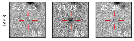
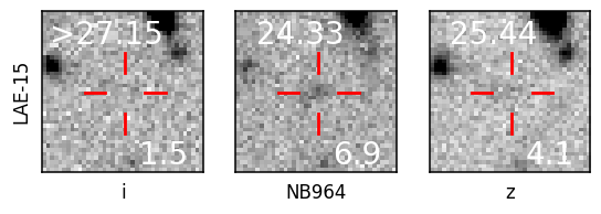
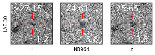
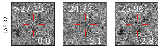
We find 39 sources sources in the VIK J2348–3054 field which meet our selection criteria: 38 LAE candidates as well as the quasar itself. The 20 pix 20 pix (10.8” 10.8”) postage stamp cut outs of all the candidates are presented in Figure 11 in the appendix. We also indicate the magnitudes in the respective bands as well as their S/N. While all candidates formally meet our selection criteria (see Sect. 2.3), we do note that three candidates (LAE-25, LAE-30, and LAE-38) seem to have obvious i-band detections despite SExtractor assigning them very low S/N values. By contrast, only two candidates were identified in the CDFS images after the photometry degradation (see Sect. 2.3).
Our candidate properties are presented in Table 2 in the appendix, including their positions, separation from VIK J2348–3054, i-band, z-band, and NB964 magnitudes, Ly- luminosities, and star formation rates (see sections 3.2 and 3.3). VIK2348–3054 also met the selection criteria and is therefore also presented in Table 1. The z magnitude determined for the quasar is nearly 0.8 mag fainter than the one reported in Venemans et al. (2013), upon discovery, who measured a Gunn z filter magnitude of on the 3.8m New Technology Telescope (NTT). The slight difference between the two is easily explainable by the difference in filter sets between DECam and NTT; the z-band in DECam is much redder than in EFOCS2 (because of the lower efficiency of the CCD at long wavelengths). This is also notable in Table 3 of Mazzucchelli et al. (2017b) where the PS1 z-band magnitudes differ from the DECam z-band photometry by substantial amounts due to the filter curve. Additionally, our DECam z value is also expected given the relationship between previous quasars’ DECam z magnitudes and their J band magnitudes (see Table in 3 in Mazzucchelli et al., 2017a) which have comparable redshifts and luminosities to VIKJ2348-3054.
The on-sky distribution of the LAE candidates around the quasar can be seen in Figure 6.

3.2 Estimation of Ly- Luminosities
We follow the same method used by Hu et al. (2019) to determine the Ly- luminosities of our candidates. Specifically, we use the following equation to estimate the flux density from the Ly- emission line (),
| (9) | ||||
| (10) |
where is the transmission function of filter (in our case is either NB964 or the z-band), is the observed flux density, and is a constant defined as:
| (11) |
where is the central wavelength of filter and is the speed of light. For simplicity, we assume that the Ly- emission line () is a -function, centred on the NB964 filter, and the continuum flux () is a power law spectrum with a slope of -2 and attenuated by the IGM using the model from Madau (1995). Making these assumptions allows us to express Equation (10) as:
| (12) |
where is the Ly- flux, is a constant, and is the average IGM absorption optical depth at the redshift of the quasar. When we substitute the narrowband and broadband values into Equation (12) we get two equations:
| (13) | ||||
| (14) |
where is the Ly- emission wavelength. We can solve Equations 13 and 14 simultaneously for and , using the latter to determine the Ly- luminosity ().
3.3 Star formation rates
We estimate the star formation rates (SFRs) by following the same procedure used by Mazzucchelli et al. (2017a). Using the derived Ly- luminosities (), we can determine H luminosities () by assuming case-B recombination and exploiting the relationship presented in Osterbrock (1989): . SFRs can be calculated using the relationship between SFR and presented in Kennicutt & Evans (2012):
| (15) |
However, it is worth noting that these star formation rate estimates are highly uncertain given that we do not know the intrinsic Ly- luminosity due to star formation and the observed Ly- luminosity is most likely a fraction of the intrinsic total.
4 Discussion
4.1 Overdensity of LAEs
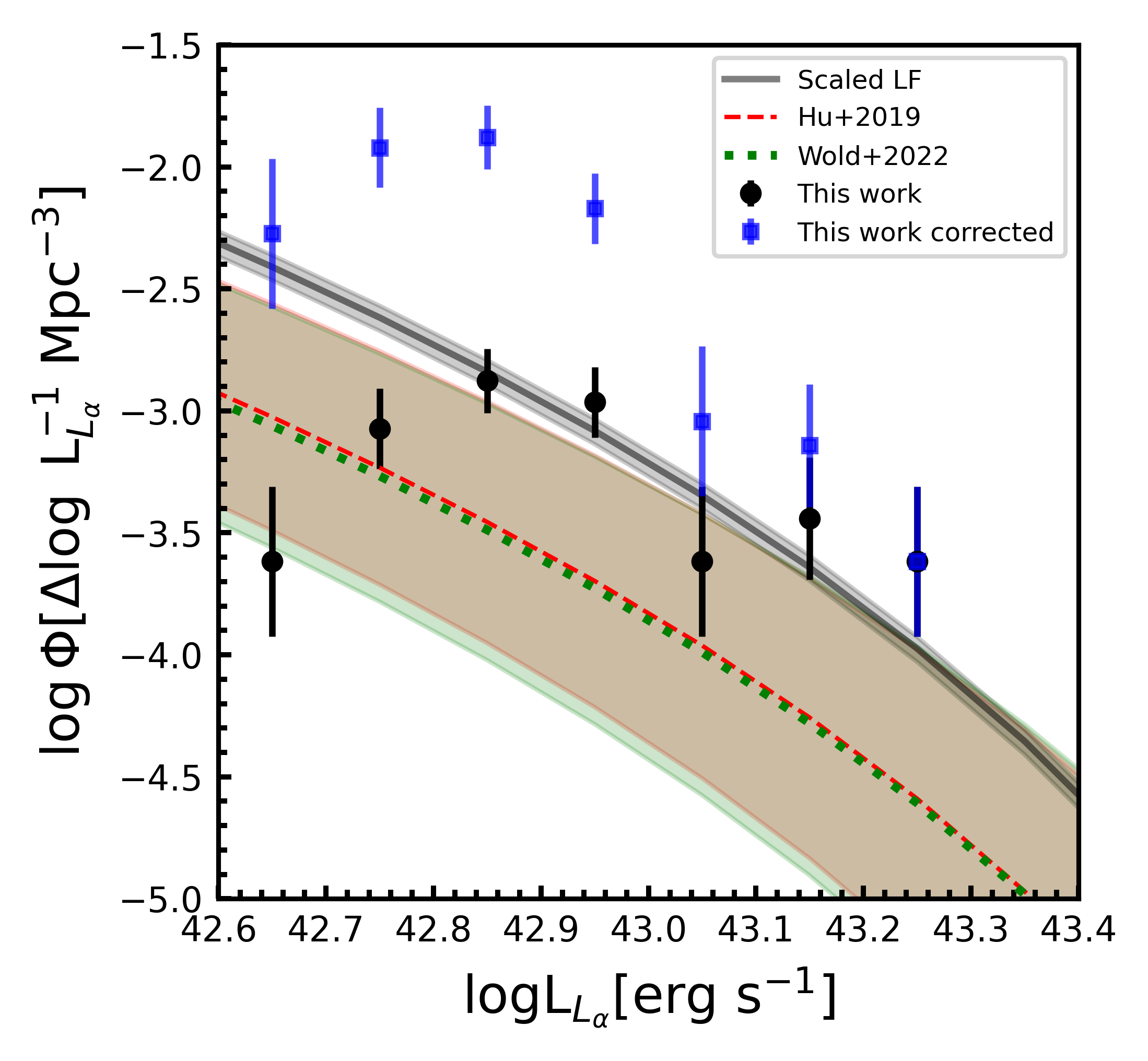
Considering the number of candidates (section 3.1) and usable area of each field (section 2), we find the surface density of LAEs around VIK J2348–3054 to be deg-2, whilst in CDFS we only find a surface density of deg-2 to the same depth (see Sect. 2.3 for details). If we define as a density consistent with a field density, then this quasar is sitting within an overdense region with an overdensity factor of , where the uncertainty corresponds to the 68 confidence interval. We note that given this highly skewed distribution, the probability of the field not being overdense (i.e, the probability that ) is 3. To further explore the overdensity factor and make sure the result is not driven by the CDFS density, we constructed a Ly- luminosity function (see the values used in Table 1) and compared it to the combined CDFS and COSMOS fields from Hu et al. (2019) and the combined LAGER 4-field luminosity function from Wold et al. (2022) in Figure 8. We define the luminosity function as:
| (16) |
where is the effective volume of our survey– cMpc3–determined by taking into account the survey area and the redshift range probed, and is the bin-width = 0.1 . We also include a detection completeness factor——as described in Hu et al. (2019) and Wold et al. (2022). This factor is calculated by inserting, and then recovering, false sources in the narrowband. The factor is shown in Figure 8 as a function of magnitude. Specifically, we use the best-fit error function shown in the Figure to estimate the luminosity function. To further constrain which equivalent widths we are sensitive to we also investigated what range of equivalent widhts would pass our selection criteria for a given Ly- luminosity. In particular: we assumed zero flux in the i-band; for each bin in Figure 8 we calculated the percentage of synthetic LAEs that would pass our selection criteria, with equivalent widths ranging from 1 - 200 ; we then divide the luminosity function by this completeness correction factor, which results in the blue points in Figure 8. Our limit-assumption correction suggests an even larger overdensity. However, the uncommon shape of the LF observed after correction suggests that there is likely a more complex distribution of EWs, and the correct LF sits in between the black and blue dots.
While the overdensity is not clear in the two faintest bins, this may be due to incompleteness from our selection function. Further observations, both deeper and in other bands (as has been done for the LAGER survey, e.g., Hu et al. 2019) are likely required to determine the source of this. To estimate , we fit the amplitude of the luminosity functions from Hu et al. (2019) and Wold et al. (2022) to our data, without considering the two faintest bins. We find that the candidates around VIK J2348–3054 have a higher space density. The luminosity functions from Hu et al. (2019) and Wold et al. (2022) are in tight agreement (as is evident in Figure 8), and both imply an overdensity of . These luminosity functions were corrected for selection incompleteness whereas our data has not been corrected in the same way. This has the consequence of the measured value representing a lower limit, which again, indicates that the quasar lives in an overdense environment.
Interestingly, we are only able to find this overdensity due to the large size of our field, as there appears to be a distinct lack of sources in the vicinity of the quasar (see Figure 6). Figure 9 shows the LAE candidates’ radial distribution from the quasar. The blue shaded region represents the average CDFS surface density of deg2, with an uncertainty determined by considering the Poisson single-sided, upper limit for (Gehrels, 1986). Radial bins with no detections have been given an upper limit of 1.846 objects which is again the upper limit for a single-sided Poisson distribution. Figure 9 also shows the maximum radius that objects are expected to collapse into a cluster at , 75 cMpc (9.5 pMpc) expected at this redshift (Overzier et al., 2009) and is also shown as the outer ring in Figure 6. Figure 9 shows that the field is overdense throughout all the area covered by our images, except within the inner 5pMpc from the quasar. We discuss this further in the next section.

| Luminosity Range | Counts | ||
|---|---|---|---|
| [erg s | Mpc-3 | Mpc-3 | |
| 42.6 – 42.7 | 2 | -3.62 | 0.31 |
| 42.7 – 42.8 | 7 | -3.07 | 0.16 |
| 42.8 – 42.9 | 11 | -2.88 | 0.13 |
| 42.9 – 43.0 | 9 | -2.96 | 0.14 |
| 43.0 – 43.1 | 2 | -3.61 | 0.31 |
| 43.1 – 43.2 | 3 | -3.44 | 0.25 |
| 43.2 – 43.3 | 2 | -3.62 | 0.31 |
| 43.3 – 43.4 | 0 | - | - |
| 43.4 – 43.5 | 2 | -3.62 | 0.31 |
| 43.5 – 43.6 | 0 | - | - |
| 43.6 – 43.7 | 0 | - | - |

4.2 Central suppression of Ly- emitters
Figure 6 shows the on-sky distribution of LAE candidates. The inner shaded region represents the quasar proximity zone—the theoretical region around a quasar where its UV radiation would have ionized a pure hydrogen ISM (Fan et al., 2006). Mazzucchelli et al. (2017b) determined the radius of the proximity zone of VIK J2348–3054 to be 2.64 pMpc. The Figure also shows ring with the largest radius that Overzier et al. (2009) found to contain overdensities. It is worth noting that there is a small observational artifact in the form of striations, to the south of the quasar, which overlaps the proximity zone. This is caused by a relatively strong main reflection pattern in DECam, possibly by moonlight. However, the area affected is very small and this effect had no impact on LAE candidate selection.
What is striking about the on-sky distribution is the discernible lack of candidates towards the center of the image, around the quasar position (also see Figure 9). In fact, the nearest candidate to the quasar is 0.27∘ away, i.e., 5.15 pMpc. This distance is indicated by the dashed ring in Figure 6. If we take the area outside of the maximum radius at which objects are expected to collapse into clusters at , i.e, the region beyond the outer ring in Figure 6, where we do not expect the quasar to have much, if any, influence, and use it to estimate the average field density, then the Poisson probability of finding the inner region void of LAEs is 1.2. However, when coupled with the fact that this underdense region is centered on the already rare luminous high-z quasar, we can conclude it is highly unlikely that this is a chance occurrence, but instead shows a real dearth of LAEs. Furthermore, we would naively expect the quasar to be close to the center of overdensity, where the environment should be more concentrated than in the outskirts, making this underdensity even more striking. In the following sections we discuss potential explanations for this observed lack of LAEs in the vicinity of VIK 2348-3054.
4.2.1 Star formation suppression due to negative feedback
A popular mechanism previously suggested to explain a lack of LAEs around some quasars has been negative feedback from the quasar itself (Bañados et al., 2013; Morselli et al., 2014; Mazzucchelli et al., 2017a; Ota et al., 2018). In this scenario, the strong ionizing radiation from the quasar photoevaporates neutral hydrogen in its immediate vicinity, prohibiting gas condensation, and thus inhibiting star formation in galaxies where it would otherwise be able to occur (Kim et al., 2009; Overzier et al., 2009). Our results are consistent with the expected scale proposed by a variety of studies (e.g., Chen, 2020; Zhou et al., 2023), all suggesting that this effect should be within pMpc. We further quantify this by calculating the isotropic UV intensity in a sphere around the quasar, following Kashikawa et al. (2007), and determine the local flux density at different distances from the quasar via:
| (17) |
where is the distance from the quasar and is the quasar luminosity at the Lyman limit (912Å). The latter can be estimated as in Mazzucchelli et al. (2017b) by using the extinction-corrected rest-frame 1450 Å AB magnitude:
| (18) |
where is the luminosity distance to the quasar, is the extinction-corrected rest-frame 1450 Å AB magnitude, is 3631 Jy, and is the continuum slope (Fan et al., 2001).
We use the value of mag estimated by Mazzucchelli et al. (2017b) for VIK 2348–3054 by extrapolating from the observed J-band magnitude. We also adopt following Kashikawa et al. (2007). Using Equations (17) and (18) we determine the local flux density at 2 pMpc and 5 pMpc to be:
| (19) |
and
| (20) |
The isotropic UV intensity at the Lyman limit is then and at 2 pMpc and 5 pMpc respectively, where erg cm-2 s-1 Hz-1 sr-1 and is the UV intensity at the Lyman limit, determined by dividing the local flux density by sr.
Several simulations suggest that the is sufficient to completely inhibit star formations in haloes of mass below (Thoul & Weinberg, 1996; Kashikawa et al., 2007; Chen, 2020). Given this, and the values we determined for , it is physically possible these LAEs have been suppressed within the quasar proximity zone—2.64 pMpc (Mazzucchelli et al., 2017b), shown by the shaded region in Figure 6—up to where we find the first LAE at 5 pMpc. However, for higher mass haloes, star formation wouldn’t be suppressed; the heating caused by the ionizing radiation would be considerably less (an order of magnitude) than that of the high-mass collapsing gas cloud (Thoul & Weinberg, 1996). Therefore in the case of Lyman Break Galaxies (LBGs), which are generally accepted to have formed earlier and to be of larger mass than LAEs (Kashikawa et al., 2007) the effects of star formation suppression due to ionizing photons from the quasar should be smaller, if not entirely negligible. Given this, if the hole around the center is indeed caused by negative feedback, then an LBG search in the same field should reveal an overdensity of LBGs in general and populate the inner 5 pMpc around the quasar in particular.
Different quasar properties would influence the total observable suppression. This might explain the diversity of results within the literature, for example, a more luminous quasar would be able to ionize higher mass haloes. Another factor would be the age of the quasar and the light travel time. Quasars need time to ionize their surroundings. The longer the quasar has been turned on, the larger the suppression radius, up until . Finally, the covering factor of the quasar ( along with the orientation of the host galaxy, or how off-centered the quasar is) would directly influence how many ionizing photons could escape the AGN and affect the IGM. Therefore we would expect a relationship between covering factor and overdensity.
4.2.2 Cosmic variance
Another explanation for the lack of Ly- emitters in the proximity of the quasar is cosmic variance; a chance arrangement of LAEs, without a physical cause. Indeed, this reason has been suggested by many studies to account for a lack of LAE concentrations around other high-redshift quasars (Bañados et al., 2013; Mazzucchelli et al., 2017a; Ota et al., 2018). Although in the previous section we concluded it is very unlikely that the underdensity around VIK 2348-3054 is caused by chance, we cannot completely rule out this possibility. Interestingly Chen (2020), using an adaptive refinement tree code on a suite of simulations, showed that the lack of faint galaxies due to suppression of star formation from quasars was a less important factor on the cumulative luminosity function than simple field-to-field variation. They determined this by searching for LAEs in random 1 pMpc radii spheres in simulations. Their results suggest that cosmic variance is an effect which needs to be considered seriously in this context. Accounting for cosmic variance robustly would require further comparisons, on similar depths and FoVs, to other blank fields as well as wider field of view observations of other quasar fields. In contrast to star formation suppression, LBGs would be expected to show a similar pattern as LAEs around VIK J2348–3054 if the observed structure is a result of cosmic variance.
4.2.3 Sensitivity
As mentioned, suppression of Ly- emission should occur in galaxies with halo masses less than . However, if a survey is unable to detect faint LAEs which fall into this regime, then it is possible that the faint LAEs do exist around the central quasar, but are just undetected. It is important to note that there have been confirmed detections of LAEs near quasars that LAEs near quasars have been spectroscopically confirmed using JWST Iani et al. (2024). This suggests that follow up observations at much higher sensitivities, possibly using JWST, are needed. However, if sensitivity were the reason for the lack of detected LAEs around VIKJ2348–3054 then this would then raise the question as to why we don’t detect any high-mass LAEs in the immediate vicinity of the quasar. So while sensitivity is an important component to consider, it does not fully explain our observed distribution of LAEs.
4.2.4 Other possible physical mechanisms
The lack of central LAEs near the quasar might be physically driven by processes other than star formation suppression by the quasar and cosmic variance.
A merging scenario was suggested by Bañados et al. (2013). In this model, the central quasar grows its mass through hierarchical mergers with surrounding haloes, creating an underdensity in its vicinity. This scenario would also potentially explain the quick SMBH growth experienced by high-redshift quasars and, at the same time, explains the apparent lack of the LAEs in the nearby vicinity as they would have merged with the host galaxy of the quasar.
On the other hand, Willott et al. (2005), Kim et al. (2009), and Mazzucchelli et al. (2017a), raised the possibility that candidates around the quasar might be dust obscured, thereby resulting in non-detections. However, explaining our results would require a gradient in the amount of dust as a function of the distance to the quasar, which seems unlikely. Submm interferometric surveys within the inner 5 pMpc might be able to confirm or deny this effect. Although, mapping such a large area with, e.g., ALMA, would be observationally expensive. For example, ALMA observations of VIK J2348–3054 by Venemans et al. (2016), which cover an area of only 0.13 arcmin2 area, found no companion galaxies. Recently, Li et al. (2023) searched for submm galaxies around quasars—including VIK J2348–3054—using the Submillimeter Common-User Bolometre Array-2 (SCUBA-2) on the James Clerk Maxwell Telescope, which has a much larger 15’ field-of-view. This field of view translates to 5pMpc. Li et al. (2023) only found a single SMG around VIK J2348–3054, 0.5 pMpc away from the quasar, suggesting that dust obscuration may not be the cause of the central lack of LAEs.
Whilst these suggested mechanisms may be reasonable to explain the results of individual observations, they fail to account for the breadth of results throughout the literature—underdensities, field-densities, and overdensities. Considering this, we conclude that negative feedback is the most likely explanation of the observed results in this work.
4.3 Comparison to other studies
The varying results throughout the literature have been difficult to constrain and many explanations have been given for the scatter. In Figure 10 we summarize the results of previous studies that targeted 20 quasars in the redshift range to , that searched for either LAEs or LBGs in their vicinity. Specifically, we show the search area and the value of determined by each study.
Of the 20 quasars only six were searched for neighboring LAEs. And of these six observations, none found overdensities. Furthermore there were no multiple LAE searches done on any of these quasars, meaning that only six LAE searches were done in total (Bañados et al., 2013; Mazzucchelli et al., 2017a; Kikuta et al., 2017; Goto et al., 2017; Ota et al., 2018). On the other hand, 16 of the quasars had LBG surveys done, and some quasars were studied multiple times by different groups. In total there were 24 LBG searches done, of which 16 (67) found overdensities, whilst 8 (33) did not. The fact that many LAE searches don’t detect overdensities, whilst at the same time, most LBG searches do, suggests that quasars may be suppressing star-formation in their environments. As we mentioned previously, the younger, lower mass LAEs would be more affected than the older, higher mass LBGs. Therefore, we would expect to find less overdensities when looking for LAEs. Alternatively, narrowband imaging might not have enough sensitivity if the equivalent widths are low.
Several quasars have had both LAEs and LBGs searches done. VIKJ1030–0524 was investigated for LBGs by Morselli et al. (2014) and Balmaverde et al. (2017). Later, Mignoli et al. (2020) performed spectroscopy using MUSE at VLT and spectroscopically identified the LBGs within their FoV, and found two LAE within 5 pMpc of the quasar. Mignoli et al. (2020) themselves note that the low number of detected LAEs close to the quasar may be hinting at negative feedback; confirming an overdensity in general but lacking in LAEs.
Ota et al. (2018) searched for both LBGs and LAEs around VIK J0305–3150 and found, at low masses, a slight overdensity of LBGs and an underdensity of LAEs. Later, Champagne et al. (2023) reported a massive overdensity of LBGs very near the same quasar. Whilst narrowband searches for LAEs around the quasar have resulted in non-detections, spectroscopic observations, in particular with MUSE on the Very Large Telescope, identified a LAE very near to the quasar (Farina et al., 2017). Recently, James Webb Space Telescope (JWST) slitless spectroscopy has identified 10 [OIII] emitting galaxies, which trace a filamentary structure around this quasar (Wang et al., 2023). These results highlight the importance that spectroscopic follow up can play in determining overdensities.
Utsumi et al. (2010) and Goto et al. (2017) both observed CFHQS J2329–0301 for LBGs and LAEs respectively, with Subaru/Suprime-Cam. Once again, the quasar had an overdensity of LBGs and an underdensity of LAEs.
Bañados et al. (2013) and Mazzucchelli et al. (2017a) searched for LAEs around ULAS J0203+0012 and PSO J215.1512–16.0417 respectively, and also performed Lyman-break selections around their respective targets. They found that the number of LBG candidates was consistent with blank fields. It is worth noting that both used the FOcal Reducer/low dispersion Spectrograph 2 (FORS2) on the Very Large Telescope (VLT) which has a FoV of 37 arcmin2 and they did not use an optimum filter set up, which may have influenced results.
Recently, Champagne et al. (2023) performed an LBG search around the target of our study for LAEs—VIK J2348–3054—using the Advanced Camera for Surveys (ACS) onboard the Hubble Space Telescope (HST). Whilst they claim no LBG enhancement, they still find 10 LBG candidates within 0.3 pMpc, well within the quasar proximity zone (5 secure detections and 5 marginal detections). On the other hand, we do not find any LAEs within a much larger area around VIK J2348–3054. Once again, the lack of LAE and the detection of LBGs is expected, further hinting at star formation suppression.
There is also evidence at lower redshifts () which suggest a similar effect might be occurring. Specifically, García-Vergara et al. (2017) used a custom set of narrowband filters which were optimized for identifying LBGs around six quasars; the QSO-LBG cross-correlation function showed an overdensity. Later, García-Vergara et al. (2019) performed a similar work, but for LAEs around 17 quasars and again the QSO-LAE cross-correlation function found an overdensity. However, the LBG overdensity signal was stronger than the LAE one by a factor of 10 (see the bottom panel of Figure 6 in García-Vergara et al., 2022).
The notion of LAE suppression due to the quasar seems to explain a lot of the results throughout the literature. However, at the same time, our study is the only one which has found an overdensity of LAEs around a high-redshift quasar () using the narrowband search technique. And is the largest area ever searched for either LBGs or LAEs (see the solid purple star in Figure 10). Moreover, had we observed VIK J2348–3054 with any other observational set up, on any of the other telescopes that were used in previous observations, we would not have detected an overdensity. This would seem to suggest that the lack of overdensities of LAEs in previous studies might have been due to not probing a large enough area, and wider FoV studies would possibly have revealed overdense regions.

5 Summary and Conclusion
In this paper we aimed to address important observational factors we believe have influenced previous studies which searched for overdensities around high-redshift quasars. Specifically, we searched for LAEs over an area of 3.26 deg2, much larger than that probed by previous studies (see Figure 10), constituting the largest FoV searched for LAEs or LBGs around a high-redshift quasar to date. Additionally, we use a narrow-band that covers Ly- at the systemic redshift of a quasar determined from [CII] observations, to avoid biases due to uncertain redshift estimates from, e.g., CIV and MgII (see Decarli et al., 2018).
We found 38 LAE candidates around VIK J2348–3054 and applied our same selection criteria to the CDFS, images obtained with the same setup by Hu et al. (2019), for comparison. After degrading the CDFS data to match our shallower depths, we found only two LAE candidates. Adjusting for the differences in the usable areas of both fields, this implies that VIK J2348–3054 resides in an environment that is overdense by a factor of . The space density of our candidates also sit well above the luminosity functions of both Hu et al. (2019) and Wold et al. (2022) by a factor of = 40.5, further supporting the presence of a large overdensity.
Interestingly, we identified a distinct lack of LAEs in the immediate vicinity around the quasar itself, within 5.15 pMpc. Assuming that the surface density at distances further than 75 cMpc (Overzier et al., 2009) as representative for the field, we find that the lack of LAEs withing 5.15 pMpc of the quasar has a probability of only 1.2 of occurring by chance, which is not enough to exclude cosmic variance as a cause. However, given that the underdensity is centered on the quasar itself, we take this to be a conservative estimate and while we cannot completely rule out cosmic variance, we conclude that this suppression is more likely due to a physical mechanism associated with the quasar, and propose it to be because of ionizing radiation which is inhibiting star formation in nearby ( pMpc) galaxies. We calculate the isotropic UV intensity at the Lyman limit at 5 pMpc for VIK J2348–3054 and show that this would be sufficient to suppress star formation in low mass galaxies such as LAEs but wouldn’t be enough to suppress it in larger galaxies like LBGs. It is therefore interesting that a recent small-FoV search for LBGs around VIK J2348–3054 found 10 LBG candidates within 0.3 pMpc (Champagne et al., 2023).
As shown in Figure 10, there is a wide-spread of results for studies on the environmental density of high redshift quasars. Based on the results of our study, we potentially attribute this to a variety of factors. If the quasar is indeed suppressing star formation in its nearby vicinity then that suppression would be dependent on the luminosity, age, and covering factor of the quasar, and the combination of one or any of these factors could induce a spread of results. Alternatively, smaller FoV studies may be dominated by cosmic variance. They might also be probing areas of star-formation suppression, therefore adding to the confusion of whether quasars live in overdense environments.
Follow up observations of this field will be essential; LBG searches in particular, as well as spectroscopic follow up will help differentiate between cosmic variance and suppression of star formation.
This work has highlighted the importance of large-FoV studies and how not probing a large enough area might result in false non-detections of overdensities. It is therefore critical to perform large-FoV follow up surveys of other quasar fields, not only to cover regions much wider than those where star-formation might be suppressed by the quasar, but also to investigate the role that cosmic variance has on these kinds of surveys. It is also clear that future searches will require consistent methodologies to observationally confirm whether or not quasars live in overdense regions. Therefore, a large-FoV campaign to observe multiple high-redshift quasars would be invaluable.
Acknowledgements.
We thank the anonymous referee for the valuable comments. Based on observations at Cerro Tololo Inter-American Observatory, NSF’s NOIRLab (NOIRLab Prop. ID 2021B-0905; PI: R. Assef), which is managed by the Association of Universities for Research in Astronomy (AURA) under a cooperative agreement with the National Science Foundation. TSL, RJA, and AP acknowledge support from grant CONICYT + PCI + INSTITUTO MAX PLANCK DE ASTRONOMIA MPG190030. RJA acknowledge support from ANID BASAL project FB210003. RJA was supported by FONDECYT grant numbers 1191124 and 123171, and by the ANID BASAL project FB210003. CM acknowledges support from Fondecyt Iniciacion grant 11240336 and the ANID BASAL project FB210003. JXW acknowledges support from the science research grant from the China Manned Space Project with No. CMS-CSST-2021-A07.References
- Abbott et al. (2021) Abbott, T. M. C., Adamów, M., Aguena, M., et al. 2021, ApJS, 255, 20
- Angulo et al. (2012) Angulo, R. E., Springel, V., White, S. D. M., et al. 2012, MNRAS, 425, 2722
- Bañados et al. (2013) Bañados, E., Venemans, B., Walter, F., et al. 2013, ApJ, 773, 178
- Balmaverde et al. (2017) Balmaverde, B., Gilli, R., Mignoli, M., et al. 2017, A&A, 606, A23
- Bertin & Arnouts (1996) Bertin, E. & Arnouts, S. 1996, A&AS, 117, 393
- Bosman et al. (2022) Bosman, S. E. I., Davies, F. B., Becker, G. D., et al. 2022, MNRAS, 514, 55
- Capak et al. (2011) Capak, P. L., Riechers, D., Scoville, N. Z., et al. 2011, Nature, 470, 233
- Chambers et al. (2016) Chambers, K. C., Magnier, E. A., Metcalfe, N., et al. 2016, arXiv e-prints, arXiv:1612.05560
- Champagne et al. (2023) Champagne, J. B., Casey, C. M., Finkelstein, S. L., et al. 2023, ApJ, 952, 99
- Chen (2020) Chen, H. 2020, ApJ, 893, 165
- Chiang et al. (2017) Chiang, Y.-K., Overzier, R. A., Gebhardt, K., & Henriques, B. 2017, ApJ, 844, L23
- Costa et al. (2014) Costa, T., Sijacki, D., Trenti, M., & Haehnelt, M. G. 2014, MNRAS, 439, 2146
- Decarli et al. (2019) Decarli, R., Mignoli, M., Gilli, R., et al. 2019, A&A, 631, L10
- Decarli et al. (2018) Decarli, R., Walter, F., Venemans, B. P., et al. 2018, ApJ, 854, 97
- Díaz-Santos et al. (2021) Díaz-Santos, T., Assef, R. J., Eisenhardt, P. R. M., et al. 2021, A&A, 654, A37
- Eilers et al. (2023) Eilers, A.-C., Simcoe, R. A., Yue, M., et al. 2023, ApJ, 950, 68
- Fan et al. (2023) Fan, X., Bañados, E., & Simcoe, R. A. 2023, ARA&A, 61, 373
- Fan et al. (2006) Fan, X., Strauss, M. A., Becker, R. H., et al. 2006, AJ, 132, 117
- Fan et al. (2001) Fan, X., Strauss, M. A., Richards, G. T., et al. 2001, AJ, 121, 31
- Farina et al. (2022) Farina, E. P., Schindler, J.-T., Walter, F., et al. 2022, ApJ, 941, 106
- Farina et al. (2017) Farina, E. P., Venemans, B. P., Decarli, R., et al. 2017, ApJ, 848, 78
- Flaugher et al. (2015) Flaugher, B., Diehl, H. T., Honscheid, K., et al. 2015, AJ, 150, 150
- Gaia Collaboration et al. (2018) Gaia Collaboration, Brown, A. G. A., Vallenari, A., et al. 2018, A&A, 616, A1
- García-Vergara et al. (2019) García-Vergara, C., Hennawi, J. F., Barrientos, L. F., & Arrigoni Battaia, F. 2019, ApJ, 886, 79
- García-Vergara et al. (2017) García-Vergara, C., Hennawi, J. F., Barrientos, L. F., & Rix, H.-W. 2017, ApJ, 848, 7
- García-Vergara et al. (2022) García-Vergara, C., Rybak, M., Hodge, J., et al. 2022, ApJ, 927, 65
- Gehrels (1986) Gehrels, N. 1986, ApJ, 303, 336
- Goto et al. (2017) Goto, T., Utsumi, Y., Kikuta, S., et al. 2017, MNRAS, 470, L117
- Hu et al. (2019) Hu, W., Wang, J., Zheng, Z.-Y., et al. 2019, ApJ, 886, 90
- Husband et al. (2013) Husband, K., Bremer, M. N., Stanway, E. R., et al. 2013, MNRAS, 432, 2869
- Iani et al. (2024) Iani, E., Caputi, K. I., Rinaldi, P., et al. 2024, ApJ, 963, 97
- Inayoshi et al. (2020) Inayoshi, K., Visbal, E., & Haiman, Z. 2020, ARA&A, 58, 27
- Kashikawa et al. (2007) Kashikawa, N., Kitayama, T., Doi, M., et al. 2007, ApJ, 663, 765
- Kennicutt & Evans (2012) Kennicutt, R. C. & Evans, N. J. 2012, ARA&A, 50, 531
- Khostovan et al. (2020) Khostovan, A. A., Malhotra, S., Rhoads, J. E., et al. 2020, MNRAS, 493, 3966
- Kikuta et al. (2017) Kikuta, S., Imanishi, M., Matsuoka, Y., et al. 2017, ApJ, 841, 128
- Kim et al. (2009) Kim, S., Stiavelli, M., Trenti, M., et al. 2009, ApJ, 695, 809
- Li et al. (2023) Li, Q., Wang, R., Fan, X., et al. 2023, ApJ, 954, 174
- Madau (1995) Madau, P. 1995, ApJ, 441, 18
- Malhotra & Rhoads (2002) Malhotra, S. & Rhoads, J. E. 2002, ApJ, 565, L71
- Matthee et al. (2015) Matthee, J., Sobral, D., Santos, S., et al. 2015, MNRAS, 451, 400
- Mazzucchelli et al. (2017a) Mazzucchelli, C., Bañados, E., Decarli, R., et al. 2017a, ApJ, 834, 83
- Mazzucchelli et al. (2017b) Mazzucchelli, C., Bañados, E., Venemans, B. P., et al. 2017b, ApJ, 849, 91
- Mazzucchelli et al. (2023) Mazzucchelli, C., Bischetti, M., D’Odorico, V., et al. 2023, A&A, 676, A71
- Mignoli et al. (2020) Mignoli, M., Gilli, R., Decarli, R., et al. 2020, A&A, 642, L1
- Morselli et al. (2014) Morselli, L., Mignoli, M., Gilli, R., et al. 2014, A&A, 568, A1
- Osterbrock (1989) Osterbrock, D. E. 1989, Astrophysics of gaseous nebulae and active galactic nuclei
- Ota et al. (2018) Ota, K., Venemans, B. P., Taniguchi, Y., et al. 2018, ApJ, 856, 109
- Ouchi et al. (2020) Ouchi, M., Ono, Y., & Shibuya, T. 2020, ARA&A, 58, 617
- Overzier et al. (2009) Overzier, R. A., Guo, Q., Kauffmann, G., et al. 2009, MNRAS, 394, 577
- Polletta et al. (2007) Polletta, M., Tajer, M., Maraschi, L., et al. 2007, ApJ, 663, 81
- Schindler et al. (2020) Schindler, J.-T., Farina, E. P., Bañados, E., et al. 2020, ApJ, 905, 51
- Simpson et al. (2014) Simpson, C., Mortlock, D., Warren, S., et al. 2014, MNRAS, 442, 3454
- Stiavelli et al. (2005) Stiavelli, M., Djorgovski, S. G., Pavlovsky, C., et al. 2005, ApJ, 622, L1
- Thoul & Weinberg (1996) Thoul, A. A. & Weinberg, D. H. 1996, ApJ, 465, 608
- Utsumi et al. (2010) Utsumi, Y., Goto, T., Kashikawa, N., et al. 2010, ApJ, 721, 1680
- Valdes et al. (2014) Valdes, F., Gruendl, R., & DES Project. 2014, in Astronomical Society of the Pacific Conference Series, Vol. 485, Astronomical Data Analysis Software and Systems XXIII, ed. N. Manset & P. Forshay, 379
- Venemans et al. (2013) Venemans, B. P., Findlay, J. R., Sutherland, W. J., et al. 2013, ApJ, 779, 24
- Venemans et al. (2007) Venemans, B. P., McMahon, R. G., Warren, S. J., et al. 2007, MNRAS, 376, L76
- Venemans et al. (2016) Venemans, B. P., Walter, F., Zschaechner, L., et al. 2016, ApJ, 816, 37
- Verhamme et al. (2018) Verhamme, A., Garel, T., Ventou, E., et al. 2018, MNRAS, 478, L60
- Volonteri (2012) Volonteri, M. 2012, Science, 337, 544
- Wang et al. (2021) Wang, F., Yang, J., Fan, X., et al. 2021, ApJ, 907, L1
- Wang et al. (2023) Wang, F., Yang, J., Hennawi, J. F., et al. 2023, ApJ, 951, L4
- Willott et al. (2010) Willott, C. J., Delorme, P., Reylé, C., et al. 2010, AJ, 139, 906
- Willott et al. (2005) Willott, C. J., Percival, W. J., McLure, R. J., et al. 2005, ApJ, 626, 657
- Wold et al. (2019) Wold, I. G. B., Kawinwanichakij, L., Stevans, M. L., et al. 2019, ApJS, 240, 5
- Wold et al. (2022) Wold, I. G. B., Malhotra, S., Rhoads, J., et al. 2022, ApJ, 927, 36
- Yang et al. (2023) Yang, J., Wang, F., Fan, X., et al. 2023, ApJ, 951, L5
- Zewdie et al. (2023) Zewdie, D., Assef, R. J., Mazzucchelli, C., et al. 2023, A&A, 677, A54
- Zheng et al. (2006) Zheng, W., Overzier, R. A. asnd Bouwens, R. J., White, R. L., et al. 2006, ApJ, 640, 574
- Zheng et al. (2019) Zheng, Z.-Y., Rhoads, J. E., Wang, J.-X., et al. 2019, PASP, 131, 074502
- Zheng et al. (2017) Zheng, Z.-Y., Wang, J., Rhoads, J., et al. 2017, ApJ, 842, L22
- Zhou et al. (2023) Zhou, Y., Chen, H., Di Matteo, T., et al. 2023, arXiv e-prints, arXiv:2309.11571
Appendix A Additional Material
| ID | R.A. | Dec. | i | z | NB964 | SFR | ||||
|---|---|---|---|---|---|---|---|---|---|---|
| (J2000.00) | (J2000.00) | (deg) | (cMpc) | (pMpc) | (ergs s-1) | ( yr-1) | ||||
| QSO | 23:48:33.33 | -30:54:10.23 | 0.00 | 0.00 | 0.00 | >27.15 | 22.19 0.05 | 20.86 0.01 | - | - |
| LAE-1 | 23:50:39.46 | -31:47:26.41 | 0.99 | 149.20 | 18.89 | >27.15 | 24.97 0.16 | 24.11 0.12 | 7.6 2.7 | 4.7 1.7 |
| LAE-2 | 23:49:25.39 | -31:46:34.95 | 0.89 | 133.93 | 16.95 | >27.15 | 26.07 0.43 | 24.73 0.22 | 6.6 2.7 | 4.1 1.7 |
| LAE-3 | 23:49:45.53 | -31:39:01.46 | 0.79 | 118.57 | 15.01 | >27.15 | 25.74 0.33 | 24.59 0.19 | 6.6 2.8 | 4.0 1.7 |
| LAE-4 | 23:48:22.23 | -31:37:53.92 | 0.73 | 109.47 | 13.86 | >27.15 | 25.93 0.38 | 24.46 0.17 | 9.0 2.7 | 5.5 1.7 |
| LAE-5 | 23:48:17.08 | -31:30:18.94 | 0.61 | 90.77 | 11.49 | >27.15 | 26.09 0.45 | 23.59 0.07 | 26.5 2.7 | 16.4 1.7 |
| LAE-6 | 23:46:51.65 | -31:19:29.93 | 0.56 | 83.48 | 10.57 | >27.15 | 25.85 0.36 | 24.37 0.16 | 9.8 2.8 | 6.1 1.7 |
| LAE-7 | 23:52:04.95 | -31:16:20.60 | 0.84 | 126.08 | 15.96 | >27.15 | 25.38 0.24 | 23.50 0.07 | 25.5 2.8 | 15.7 1.7 |
| LAE-8 | 23:44:51.34 | -31:14:01.78 | 0.86 | 128.78 | 16.30 | >27.15 | 25.99 0.42 | 24.08 0.12 | 15.0 2.8 | 9.2 1.7 |
| LAE-9 | 23:49:09.11 | -31:11:23.68 | 0.31 | 47.13 | 5.97 | >27.15 | 25.84 0.36 | 24.53 0.18 | 7.7 2.8 | 4.8 1.7 |
| LAE-10 | 23:48:38.18 | -31:10:25.49 | 0.27 | 40.72 | 5.15 | >27.15 | 26.12 0.47 | 24.49 0.18 | 9.4 2.8 | 5.8 1.7 |
| LAE-11 | 23:52:11.44 | -31:10:09.82 | 0.82 | 123.43 | 15.62 | >27.15 | 25.55 0.28 | 24.47 0.18 | 6.9 2.8 | 4.2 1.8 |
| LAE-12 | 23:50:09.67 | -31:00:28.43 | 0.36 | 53.98 | 6.83 | >27.15 | 25.54 0.28 | 24.20 0.14 | 10.7 2.8 | 6.6 1.7 |
| LAE-13 | 23:52:50.08 | -30:59:23.05 | 0.92 | 138.21 | 17.50 | >27.15 | 25.81 0.36 | 24.37 0.16 | 9.7 2.9 | 6.0 1.8 |
| LAE-14 | 23:46:52.33 | -30:57:07.02 | 0.36 | 54.65 | 6.92 | >27.15 | 26.07 0.44 | 24.66 0.22 | 7.3 2.8 | 4.5 1.7 |
| LAE-15 | 23:52:39.27 | -30:51:50.73 | 0.88 | 132.02 | 16.71 | >27.15 | 25.44 0.27 | 24.32 0.16 | 8.1 2.9 | 5.0 1.8 |
| LAE-16 | 23:51:42.32 | -30:50:46.97 | 0.68 | 101.71 | 12.87 | >27.15 | 25.33 0.23 | 24.46 0.16 | 5.5 2.7 | 3.4 1.7 |
| LAE-17 | 23:45:30.76 | -30:50:42.20 | 0.66 | 98.31 | 12.44 | >27.15 | 25.86 0.37 | 24.72 0.22 | 5.8 2.8 | 3.6 1.7 |
| LAE-18 | 23:45:38.56 | -30:41:06.23 | 0.66 | 99.34 | 12.57 | >27.15 | 25.69 0.32 | 24.28 0.14 | 10.4 2.7 | 6.4 1.7 |
| LAE-19 | 23:50:56.96 | -30:40:16.95 | 0.56 | 84.55 | 10.70 | >27.15 | 26.03 0.43 | 24.07 0.12 | 15.3 2.8 | 9.5 1.7 |
| LAE-20 | 23:46:20.25 | -30:40:03.94 | 0.53 | 79.67 | 10.08 | >27.15 | 25.38 0.24 | 24.57 0.19 | 4.6 2.8 | 2.8 1.7 |
| LAE-21 | 23:48:12.27 | -30:32:34.32 | 0.37 | 55.15 | 6.98 | >27.15 | 26.02 0.42 | 24.22 0.14 | 12.9 2.8 | 7.9 1.7 |
| LAE-22 | 23:44:45.07 | -30:31:07.12 | 0.90 | 135.50 | 17.15 | >27.15 | 26.05 0.45 | 24.52 0.18 | 8.8 2.8 | 5.4 1.7 |
| LAE-23 | 23:47:37.50 | -30:28:28.35 | 0.47 | 70.89 | 8.97 | >27.15 | 25.53 0.27 | 24.60 0.20 | 5.2 2.8 | 3.2 1.7 |
| LAE-24 | 23:44:31.64 | -30:27:35.79 | 0.97 | 145.88 | 18.47 | >27.15 | 25.39 0.24 | 24.41 0.17 | 6.6 2.8 | 4.1 1.8 |
| LAE-25 | 23:47:38.55 | -30:25:47.75 | 0.51 | 76.79 | 9.72 | >27.15 | 25.33 0.23 | 24.49 0.18 | 5.1 2.8 | 3.2 1.7 |
| LAE-26 | 23:44:36.91 | -30:25:04.43 | 0.98 | 146.42 | 18.53 | >27.15 | 25.95 0.40 | 23.97 0.11 | 17.0 2.8 | 10.5 1.7 |
| LAE-27 | 23:48:21.02 | -30:24:04.19 | 0.50 | 75.52 | 9.56 | >27.15 | 26.00 0.41 | 24.52 0.18 | 8.5 2.8 | 5.3 1.7 |
| LAE-28 | 23:47:21.19 | -30:22:53.54 | 0.58 | 87.27 | 11.05 | >27.15 | 25.63 0.30 | 23.84 0.10 | 18.1 2.8 | 11.2 1.7 |
| LAE-29 | 23:46:27.28 | -30:21:51.57 | 0.70 | 105.43 | 13.35 | >27.15 | 25.52 0.27 | 24.40 0.16 | 7.6 2.8 | 4.7 1.7 |
| LAE-30 | 23:49:27.05 | -30:21:25.98 | 0.58 | 86.77 | 10.98 | >27.15 | 25.65 0.30 | 24.61 0.19 | 5.9 2.7 | 3.6 1.7 |
| LAE-31 | 23:50:27.20 | -30:21:13.39 | 0.68 | 102.61 | 12.99 | >27.15 | 25.50 0.27 | 24.26 0.14 | 9.5 2.8 | 5.8 1.7 |
| LAE-32 | 23:45:02.91 | -30:12:32.87 | 1.03 | 153.76 | 19.46 | >27.15 | 25.96 0.39 | 24.73 0.21 | 6.1 2.7 | 3.8 1.7 |
| LAE-33 | 23:49:34.65 | -30:12:40.49 | 0.73 | 108.83 | 13.78 | >27.15 | 25.66 0.31 | 24.52 0.18 | 6.9 2.8 | 4.3 1.7 |
| LAE-34 | 23:50:23.24 | -30:10:45.41 | 0.82 | 123.58 | 15.64 | >27.15 | 26.13 0.48 | 24.62 0.20 | 7.9 2.8 | 4.9 1.7 |
| LAE-35 | 23:50:45.07 | -30:05:13.35 | 0.94 | 141.41 | 17.90 | >27.15 | 25.34 0.23 | 24.32 0.15 | 7.5 2.8 | 4.6 1.7 |
| LAE-36 | 23:49:43.48 | -30:03:01.26 | 0.89 | 133.31 | 16.87 | >27.15 | 25.55 0.28 | 24.31 0.15 | 9.1 2.8 | 5.6 1.7 |
| LAE-37 | 23:50:36.54 | -30:01:46.79 | 0.98 | 146.80 | 18.58 | >27.15 | 25.45 0.25 | 24.58 0.19 | 4.9 2.8 | 3.0 1.7 |
| LAE-38 | 23:48:43.58 | -29:53:13.94 | 1.02 | 152.41 | 19.29 | >27.15 | 25.80 0.36 | 24.70 0.22 | 5.7 2.9 | 3.5 1.8 |