A Joint Learning Approach for Semi-supervised Neural Topic Modeling
Abstract
Topic models are some of the most popular ways to represent textual data in an interpret-able manner. Recently, advances in deep generative models, specifically auto-encoding variational Bayes (AEVB), have led to the introduction of unsupervised neural topic models, which leverage deep generative models as opposed to traditional statistics-based topic models. We extend upon these neural topic models by introducing the Label-Indexed Neural Topic Model (LI-NTM), which is, to the extent of our knowledge, the first effective upstream semi-supervised neural topic model. We find that LI-NTM outperforms existing neural topic models in document reconstruction benchmarks, with the most notable results in low labeled data regimes and for data-sets with informative labels; furthermore, our jointly learned classifier outperforms baseline classifiers in ablation studies.
1 Introduction
Topic models are one of the most widely used and studied text modeling techniques, both because of their intuitive generative process and interpretable results Blei (2012). Though topic models are mostly used on textual data Rosen-Zvi et al. (2012); Yan et al. (2013), use cases have since expanded to areas such as genomics modeling Liu et al. (2016) and molecular modeling Schneider et al. (2017).
Recently, neural topic models, which leverage deep generative models have been used successfully for learning these probabilistic models. A lot of this success is due to the development of variational autoencoders Rezende et al. (2014); Kingma and Welling (2014) which allow for inference of intractable distributions over latent variables through a back-propagation over an inference network. Furthermore, recent research shows promising results for Neural Topic Models compared to traditional topic models due to the added expressivity from neural representations; specifically, we see significant improvements in low data regimes Srivastava and Sutton (2017); Iwata (2021).
Joint learning of topics and other tasks have been researched in the past, specifically through supervised topic models Blei and McAuliffe (2010); Huh and Fienberg (2012); Cao et al. (2015); Wang and Yang (2020). These works are centered around the idea of a prediction task using a topic model as a dimensionality reduction tool. Fundamentally, they follow a downstream task setting (Figure 1), where the label is assumed to be generated from the latent variable (topics). On the other hand, an upstream setting would be when the input (document) is generated from a combination of the latent variable (topics) and label, which has the benefit of better directly modeling how the label affects the document, resulting in topic with additional information being injected from the label information. Upstream variants of supervised topic models are much less common, with, to the extent of our knowledge, no neural architectures to this date. Ramage et al. (2009); Lacoste-Julien et al. (2008).
Our model, the Label-Indexed Neural Topic Model (LI-NTM) stands uniquely with respect to all existing topic models. We combine the benefits of an upstream generative processes (Figure 1), label-indexed topics, and a topic model capable of semi-supervised learning and neural topic modeling to jointly learn a topic model and label classifier. Our main contributions are:
-
1.
The introduction of the first upstream semi-supervised neural topic model.
-
2.
A label-indexed topic model that allows more cohesive and diverse topics by allowing the label of a document to supervise the learned topics in a semi-supervised manner.
-
3.
A joint training framework that allows for users to tune the trade-off between document classifier and topic quality which results in a classifier that outperforms same classifier trained in an isolated setting for certain hyper-parameters.
2 Related Work
2.1 Neural Topic Models
Most past work in neural topic models focused on designing inference networks with better model specification in the unsupervised setting. One line of recent research attempts to improve topic model performance by modifying the inference network through changes to the topic priors or regularization over the latent space Miao et al. (2016); Srivastava and Sutton (2017); Nan et al. (2019). Another line of research looks towards incorporating the expressivity of word embeddings to topic models Dieng et al. (2019a, b).
In contrast to existing work on neural topic models, our approach does not mainly focus on model specification; rather, we create a broader architecture into which neural topic models of all specifications can be trained in an upstream, semi-supervised setting. We believe that our architecture will enable existing neural topic models to be used in a wider range of real-word scenarios where we leverage labeled data alongside unlabeled data and use the knowledge present in document labels to further supervise topic models. Moreover, by directly tying our topic distributions to the labels through label-indexing, we create topics that are specific to labels, making these topics more interpretable as users are directly able to glean what types of documents each of the topics are summarizing.
2.2 Downstream Supervised Topic Models
Most supervised topic models follow the downstream supervised framework introduced in s-LDA Blei and McAuliffe (2010). This framework assumes a two-stage setting in which a topic model is trained and then a predictive model for the document labels is trained independently of the topic model. Neural topic models following this framework have also been developed, with the predictive model being a discriminative layer attached to the learned topics, essentially treating topic modeling as a dimensionality reduction tool Wang and Yang (2020); Cao et al. (2015); Huh and Fienberg (2012).
In contrast to existing work, LI-NTM is an upstream generative model (Figure 2, Figure 3) following a prediction-constrained framework. The upstream setting allows us to implicitly train our classifier and topic model in a one-stage setting that is end-to-end. This has the benefit of allowing us to tune the trade-off between our classifier and topic model performance in a prediction-constrained framework, which has been shown to achieve better empirical results when latent variable models are used as a dimensionality reduction tool Hughes et al. (2018); Hope et al. ; Sharma et al. (2021). Furthermore, the upstream setting allows us to introduce the document label classifier as a latent variable, enabling our model to work in semi-supervised settings.
3 Background
LI-NTM extends upon two core ideas: Latent Dirichlet Allocation (LDA) and deep generative models. For the rest of the paper, we assume a setting where we have a document corpus of D documents, a vocabulary with V unique words, and each document having a label from the L possible labels. Furthermore let us represent as the -th word in the -th document.
3.1 Latent Dirichlet Allocation (LDA)
LDA is a probabilistic generative model for topic modeling Blei et al. (2003); Blei and McAuliffe (2010). Through the process of estimation and inference, LDA learns K topics . The generative process of LDA posits that each document is a mixture of topics with the topics being global to the entire corpus. For each document, the generative process is listed below:
-
1.
Draw topic proportions Dirichlet
-
2.
For each word in document:
-
(a)
Draw topic assignment Cat()
-
(b)
Draw word Cat()
-
(a)
-
3.
Draw responses (if supervised)
where and the parameters are estimated during inference. is a hyper-parameter that serves as a prior for topic mixture proportions. In addition we also have hyper-parameter that we use to place a dirichlet prior on our topics, Dirichlet.
3.2 Deep Generative Models
Deep Generative Models serve as the bridge between probabilistic models and neural networks. Specifically, deep generative models treat the parameters of distributions within probabilistic models as outputs of neural networks. Deep generative models fundamentally work because of the re-parameterization trick that allows for backpropogation through Monte-Carlo samples of distributions from the location-scale family. Specifically, for any distribution from the location-scale family, we have that
thus allowing differentiation with respect to .
The Variational Auto-encoder is the simplest deep generative model Kingma and Welling (2014) and it’s generative process is as follows:
where are both parameterized by neural networks with variational parameters . Inference on a variational autoencoder is done through approximating the true posterior which is often intractable with an approximation that is parametrized by a neural network.
The M2 model is the semi-supervised extension of the variational auto-encoder where the input is modeled as being generated by both a continuous latent variable and the class label as a latent variable Kingma et al. (2014). It follows the generative process below:
where is parameterizing the distribution on and are both parameterized by neural networks. We then approximate the true posterior using by saying
where is a classifier that’s used in the un-labeled case and is a neural network that takes in the true labels if available and the outputted labels from if unavailable.
4 The Label-Indexed Neural Topic Model
LI-NTM is a neural topic model that leverages the labels as a latent variable alongside the topic proportions in generating the document .
Notationally, let us denote the bag of words representation of a document as and the one-hot encoded document label as . Furthermore, we denote our latent topic proportions as and our topics are represented using a three dimensional matrix .
Under the LI-NTM, the generative process (also depicted in Figure 2) of the -th document is the following:
-
1.
Draw topic proportions
-
2.
Draw document label
-
3.
For each word in document:
-
(a)
Draw topic assignment Cat()
-
(b)
Draw word Cat()
-
(a)
In Step 1, we draw from the Logistic-Normal to approximate the Dirichlet Distribution while remaining in the location-scale family necessary for re-parameterization Blei et al. (2003). This is done obtained through:
Note that since we sample from the Logistic-Normal, we do not require the Dirichlet prior hyper-parameter .
Step 2 is unique for LI-NTM , in the unlabeled case, we sample a label from , which is the output of our classifier. In the labeled scenario, we skip step 2 and simply pass in the document label for our . Step 3 is typical of traditional LDA, but one key difference is that in step 3b we also index by the by instead of just . This step is motivated by how the M2 model extended variational autoencoders to a semi-supervised setting Kingma et al. (2014).
A key contribution of our model is the idea of label-indexing. We introduce the supervision of the document labels by having different topics for different labels. Specifically, we have different topics and we denote the -th topic for label as the dimensional vector, . Under this setting, we can envision LI-NTM as running a separate LDA for each label once we index our corpus by document labels.
Label-indexing allows us to effectively train our model in a semi-supervised setting. In the un-labeled data setting, our jointly-learned classifier, , outputs a distribution over the labels, . By computing the dot-product between and our topic matrix , this allows us to partially index into each label’s topic proportional to the classifier’s confidence and update the topics based on the unlabeled examples we are currently training on.
5 Inference and Estimation
Given a corpus of normalized bag-of-word representation of documents we aim to fit LI-NTM using variational inference in order to approximate intractable posteriors in maximum likelihood estimation Jordan et al. (1999). Furthermore, we amortize the loss to allow for joint learning of the classifier and the topic model.
5.1 Variational Inference
We begin first by looking at a family of variational distributions in modeling the untransformed topic proportions and in modeling the classifier. More specifically, is a Gaussian whose mean and variance are parameterized by neural networks with parameter and is a distribution over the labels parameterized by a MLP with parameter Kingma and Welling (2014); Kingma et al. (2014).
We use this family of variational distributions alongside our classifier to lower-bound the marginal likelihood. The evidence lower bound (ELBO) is a function of model and variational parameters and provides a lower bound for the complete data log-likelihood. We derive two ELBO-based loss functions: one for the labeled case and one for the unlabeled case and we compute a linear interpolation of the two for our overall loss function.
| (1) | ||||
| (2) |
where Equation 1 serves as our unlabeled loss and Equation 2 serves as our labeled loss. is the cross-entropy function. and are hyper-parameters on the KL and cross-entropy terms in the loss respectively.
These hyper-parameters are well motivated. is seen to be a hyper-parameter that tempers our posterior distribution over weights, which has been well-studied and shown to increase robustness to model mis-specification Mandt et al. (2016); Wenzel et al. (2020). Lower values would result in posterior distributions with higher probability densities around the modes of the posterior. Furthermore, the hyperparameter in our unlabeled loss is the core hyperparameter that makes our model fit the prediction-constrained framework, essentially allowing us to trade-off the between classifier and topic modeling performance Hughes et al. (2018). Increasing values of corresponds to emphasizing classifier performance over topic modeling performance.
We treat our overall loss as a combination of our labeled and unlabeled loss with being a hyper-parameter weighing the labeled and unlabeled loss. allows us weigh how heavily we want our unlabeled data to influence our models. Example cases where we may want high values of are when we have poor classifier performance or a disproportionate amount of unlabeled data compared to label data, causing the unlabeled loss to completely outweigh the labeled loss.
| (3) |
We optimize our loss with respect to both the model and variational parameters and leverage the reparameterization trick to perform stochastic optimization Kingma and Welling (2014). The training procedure is shown in Algorithm 1 and a visualization of a forward pass is given in Figure 3. This loss function allows us to jointly learn our classification and topic modeling elements and we hypothesize that the implicit regularization from joint learning will increase performance for both elements as seen in previous research studies Zweig and Weinshall (2013).
6 Experimental Setup
We perform an empirical evaluation of LI-NTM with two corpora: a synthetic dataset and AG News.
6.1 Baselines
We compare our topic model to the Embedded Topic Model (ETM), which is the current state of the art neural topic model that leverages word embeddings alongside variational autoencoders for unsupervised topic modeling Dieng et al. (2019a). Further details about ETM are shown in the appendix (subsection A.2). Furthermore, our baseline for our jointly trained classifier is a classifier with the same architecture outside of our jointly trained setting.
6.2 Synthetic Dataset
We constructed our synthetic data to evaluate LI-NTM in ideal and worst-case settings.
-
•
Ideal Setting: An ideal setting for LI-NTM consists of a corpus with similar word distributions for documents with the same label and very dissimilar word distributions for documents with different labels
-
•
Worst Case Setting worst-case setting for LI-NTM consists of a corpus where the label has little to no correlation with the distribution of words in a document.
Since the labels are a fundamental aspect of LI-NTM we wanted to investigate how robust LI-NTM is in a real-word setting, specifically looking at how robust it was to certain types of mis-labeled data points. By jointly training our classifier with our topic model, we hope that by properly trading off topic quality and classification quality, our model will be more robust to mis-labeled data since we are able to manually tune how much we want to depend on the data labels.
We use the same distributions to generate the documents for both the ideal and worst-case data. In particular, we consider a vocabulary with words, and a task with labels. Documents are generated from one of two distributions, and . generates documents which have many occurrences of the first 10 words in the vocabulary (and very few occurrences of the last 10 words), while does the opposite, generating documents which have many occurrences of the last 10 words in the vocabulary (and very few occurrences of the first 10 words). The distributions and have parameters which are generated randomly for each trial, although the shape of the distributions is largely the same from trial to trial.
In the ideal case, the label corresponds directly to the distribution from which the document was generated. For the worst-case data, the label is 0 if the number of words in the document is an even number, and 1 otherwise, ensuring there is little to no correlation between label and word distributions in a document. Note that in our synthetic data experiments, all of the data is labeled. The effectiveness of LI-NTM in semi-supervised domains is evaluated in our AG News experiments.
6.3 AG News Dataset
The AG News dataset is a collection of news articles collected from more than 2,000 news sources by ComeToMyHead, an academic news search engine. This dataset includes 118,000 training samples and 7,600 test samples. Each sample is a short text with a single four-class label (one of world, business, sports and science/technology).
6.4 Evaluation Metrics
To evaluate our models, we used accuracy as a metric to gauge the quality of the classifier and perplexity to gauge the quality of the model as a whole. We opted to use perplexity as it is a measure for how well the model generalizes to unseen test data.
7 Synthetic Data Experimental Results
| Total Num. Topics | ETM | Ideal LI-NTM | WC LI-NTM (V1) | WC LI-NTM (V2) | Perplexity Lower Bound |
|---|---|---|---|---|---|
| 2 | |||||
| 8 | |||||
| 20 |
| Total Num. Topics | Worst Case Labels | Ideal Case Labels |
|---|---|---|
| 2 | ||
| 8 | ||
| 20 |
We used our synthetic dataset to examine the performance of LI-NTM relative to ETM in a setting where the label strongly partitions our dataset into subsets that have distinct topics to investigate the effect and robustness of label indexing.
LI-NTM was trained on the fully labeled version of the both the ideal and worse case label synthetic dataset and ETM was trained on the same dataset with the label excluded, as ETM is a unsupervised method. We varied the number of topics in both LI-NTM and ETM to explore realistic settings and the extreme setting .
7.1 Effect of Number of Topics
Takeaway: More topics lead to better performance, especially when the label is uninformative.
First, we note that as we increase the number of topics, the performance of LI-NTM on ideal case labels, LI-NTM on worst case labels, and ETM improves as shown in Table 1. This is expected as having more topics gives the model the capacity to learn more diverse topic-word distributions which leads to an improved reconstruction. However, we note that LI-NTM trained on the worst-case labels benefits most from the increase in the number of topics.
7.2 Informative Labels
Takeaway: Label Indexing is highly effective when labels partition the dataset well.
Next, we note that LI-NTM trained on the ideal case label synthetic dataset outperforms ETM with respect to perplexity (see Table 1). This result can be attributed to the fact that LI-NTM leverages label indexing to learn the label-topic-word distribution. Since the ideal case label version of the dataset was constructed such that the label strongly partitions the dataset into two groups (each of which has a very distinct topic-word distribution), and since we had perfect classifier accuracy (the ideal case label dataset was constructed such that the classification problem was trivial), LI-NTM is able to use the output from the classifier to index into the topic-word distribution with 100% accuracy.
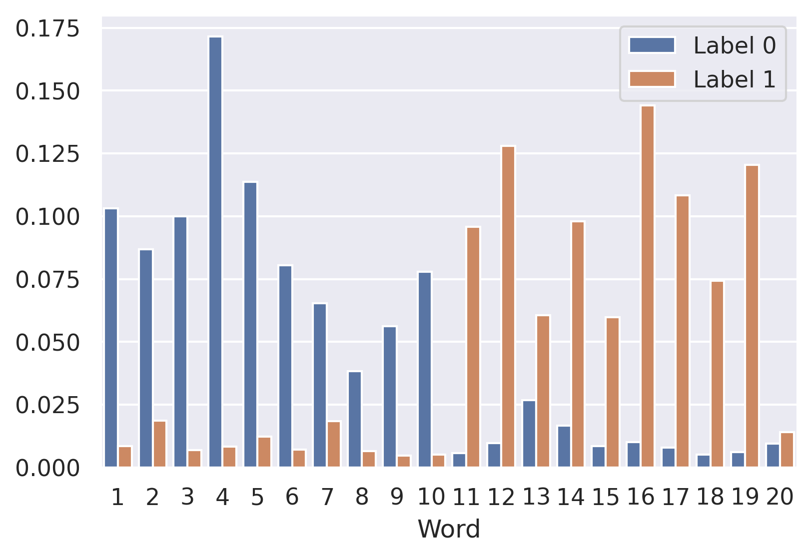
If we denote the topic-word distribution corresponding to label by and the topic-word distribution corresponding to label by , we note that LI-NTM is able to leverage to specialize in generating the words for the documents corresponding to label while using to specialize in generating the words for the documents corresponding to label (see Figure 4). Overall, this result suggests that LI-NTM performs well in settings when the dataset exhibits strong label partitioning.
7.3 Uninformative Labels
Takeaway: With proper hyperparameters, LI-NTM is able to achieve good topic model performance even when we have uninformative labels.
We now move to examining the results produced by LI-NTM trained on the worst-case labels. In this data setting, we investigated the robustness of the LI-NTM architecture. Specifically, we looked at a worst-case dataset, where we have labels that are uninformative and are thus not good at partitioning the dataset into subsets that have distinct topics.
In the worst-case setting, we define the following two instances of the LI-NTM model.
-
•
LI-NTM (V1) This model refers to the normal () version of the model trained in the worst case setting.
-
•
LI-NTM (V2) This model refers to a LI-NTM model with zero-ed out classification loss (), essentially pushing the model to only accurately reconstruct the original data.
| Data Regime | ETM Perplexity | LI-NTM Perplexity | LI-NTM Accuracy | Baseline Accuracy |
|---|---|---|---|---|
| 5% labeled, 5% unlabeled | % | % | ||
| 5% labeled, 15% unlabeled | % | % | ||
| 5% labeled, 55% unlabeled | % | % | ||
| 5% labeled, 95% unlabeled | % | % |
| Sports | Science/Technology | World | Business |
|---|---|---|---|
| series | web | minister | stocks |
| game | search | prime | oil |
| red | palestinian | prices | |
| boston | new | gaza | reuters |
| run | online | israel | company |
| night | site | leader | shares |
| league | internet | arafat | inc |
| yankees | engine | said | percent |
| new | com | yasser | yesterday |
| york | yahoo | sharon | percent |
For LI-NTM (V1), we did see decreases in performance; namely, that V1 has a worse perplexity than both ETM and ideal case LI-NTM. This aligns with our expectation that having a label with very low correlation to the topic-word distributions in the document results in poor performance in LI-NTM. This can be attributed to the failure of LI-NTM to adequately label-index in cases where this occurs.
However, for LI-NTM (V2) we found that we were actually able to achieve lower perplexity than ETM when the model was told to produce more than 2 topics, even with uninformative labels. To understand why this was happening, we analyzed the accuracy of the original classifier in LI-NTM (V2) on both the worst-case labels (which it was trained on) and the ideal-case labels (which it was not trained on). We report our results in Table 2. The key takeaway is that we observed a much higher accuracy on the ideal labels compared to the worst-case labels. This suggests that when the classifier implicitly learns the ideal labels that are necessary to learn a good reconstruction of the data, even when the provided labels are heavily uninformative or misspecified. This shows the benefit of label-indexing and of jointly learning our topic model and classifier in a semi-supervised fashion. Even in cases with uninformative data points, by setting , the joint learning setting of our classifier and topic model pushes the classifier, through the need for successful document reconstruction, to generate a probability distribution over labels that is close to the true, ideal-case labels despite only being given uninformative or mis-labeled data.
8 AG News Experimental Results
We used the AG News dataset to evaluate the performance of LI-NTM in the semi-supervised setting. Specifically, we aimed to analyze the extent to which unlabeled data can improve the performance of both the classifier and topic model in the LI-NTM architecture. Ideally, in the unlabeled case, the distant supervision provided to the classifier from the reconstruction loss would align with the task of predicting correct labels.
We ran four experiments on ETM and LI-NTM in which the amount of unlabeled data was gradually increased, while the amount of labeled data was kept fixed. In each of the experiments, 5% of the dataset was considered labeled, while 5%, 15%, 55%, and 95% of the whole dataset was considered unlabeled in each of the four experiments respectively.
8.1 Semi-Supervised Learning: Topic Model Performance
Takeaway: Combining label-indexing with semi-supervised learning increases topic model performance.
In Table 3 we observe that perplexity decreases as the model sees more unlabeled data. We also note that LI-NTM has a lower perplexity than ETM in higher data settings, supporting the hypothesis that guiding the reconstruction of a document exclusively via label-specific topics makes reconstruction an easier task. In the lowest data regime (5% labeled, 5% unlabeled), LI-NTM performs worse than ETM. This suggests that while in high-data settings, LI-NTM is able to effectively leverage sets of topics, in low-data settings there are not enough documents to learn sufficient structure.
8.2 Semi-Supervised Learning: Classifier Performance
Takeaway: Topic modeling supervises the classifier, resulting in better classification performance.
Jointly learning the classifier and topic model also seem to benefit the classifier; Table 3 shows classification performance increases linearly with the amount of unlabeled data. The accuracy increase suggest the task of reconstructing the bag of words is helpful in news article classification.
9 Conclusion
In this paper, we introduced the LI-NTM, which, to the extent of our knowledge, is the first upstream neural topic model with applications to a semi-supervised data setting. Our results show that when applied to both a synthetic dataset and AG News, LI-NTM outperforms ETM with respect to perplexity. Furthermore, we found that the classifier in LI-NTM was able to outperform a baseline that doesn’t leverage any unlabeled data. Even more promising is the fact that the classifier in LI-NTM continued to experience gains in accuracy when increasing the proportion of unlabeled data. While we aim to iterate upon our results, our current findings indicate that LI-NTM is comparable with current state-of-the-art models while being applicable in a wider range of real-world settings.
In future work, we hope to further experiment with the idea of label-indexing. While in LI-NTM every topic is label-specific, real datasets have some common words and topics that are label-agnostic. Future work could augment the existing LI-NTM framework with additional label-agnostic global topics which prevent identical topics from being learned across multiple labels. We are also interested in extending our semi-supervised, upstream paradigm to a semi-parametric setting in which the number of topics we learn is not a predefined hyperparameter but rather something that is learned.
10 Acknowledgements
AS is supported by R01MH123804, and FDV is supported by NSF IIS-1750358. All authors acknowledge insightful feedback from members of CS282 Fall 2021.
References
- Blei (2012) David M Blei. 2012. Probabilistic topic models. Communications of the ACM, 55(4):77–84.
- (2) David M Blei, Thomas L Griffiths, Michael I Jordan, Joshua B Tenenbaum, et al. Hierarchical topic models and the nested chinese restaurant process.
- Blei and Lafferty (2007) David M Blei and John D Lafferty. 2007. A correlated topic model of science. The annals of applied statistics, 1(1):17–35.
- Blei and McAuliffe (2010) David M. Blei and Jon D. McAuliffe. 2010. Supervised topic models.
- Blei et al. (2003) David M Blei, Andrew Y Ng, and Michael I Jordan. 2003. Latent dirichlet allocation. the Journal of machine Learning research, 3:993–1022.
- Cao et al. (2015) Ziqiang Cao, Sujian Li, Yang Liu, Wenjie Li, and Heng Ji. 2015. A novel neural topic model and its supervised extension. In Proceedings of the AAAI Conference on Artificial Intelligence, volume 29.
- Dieng et al. (2019a) Adji B. Dieng, Francisco J. R. Ruiz, and David M. Blei. 2019a. Topic modeling in embedding spaces.
- Dieng et al. (2019b) Adji B Dieng, Francisco JR Ruiz, and David M Blei. 2019b. The dynamic embedded topic model. arXiv preprint arXiv:1907.05545.
- Doogan and Buntine (2021) Caitlin Doogan and Wray Buntine. 2021. Topic model or topic twaddle? re-evaluating semantic interpretability measures. In Proceedings of the 2021 Conference of the North American Chapter of the Association for Computational Linguistics: Human Language Technologies, pages 3824–3848, Online. Association for Computational Linguistics.
- (10) Gabriel Hope, Michael C Hughes, Finale Doshi-Velez, and Erik B Sudderth. Prediction-constrained hidden markov models for semi-supervised classification.
- Hoyle et al. (2021) Alexander Hoyle, Pranav Goel, Andrew Hian-Cheong, Denis Peskov, Jordan Boyd-Graber, and Philip Resnik. 2021. Is automated topic model evaluation broken? the incoherence of coherence. Advances in Neural Information Processing Systems, 34.
- Hughes et al. (2018) Michael Hughes, Gabriel Hope, Leah Weiner, Thomas McCoy, Roy Perlis, Erik Sudderth, and Finale Doshi-Velez. 2018. Semi-supervised prediction-constrained topic models. In Proceedings of the Twenty-First International Conference on Artificial Intelligence and Statistics, volume 84 of Proceedings of Machine Learning Research, pages 1067–1076. PMLR.
- Huh and Fienberg (2012) Seungil Huh and Stephen E Fienberg. 2012. Discriminative topic modeling based on manifold learning. ACM Transactions on Knowledge Discovery from Data (TKDD), 5(4):1–25.
- Iwata (2021) Tomoharu Iwata. 2021. Few-shot learning for topic modeling. arXiv preprint arXiv:2104.09011.
- Jordan et al. (1999) Michael I Jordan, Zoubin Ghahramani, Tommi S Jaakkola, and Lawrence K Saul. 1999. An introduction to variational methods for graphical models. Machine learning, 37(2):183–233.
- Kingma et al. (2014) Diederik P. Kingma, Danilo J. Rezende, Shakir Mohamed, and Max Welling. 2014. Semi-supervised learning with deep generative models.
- Kingma and Welling (2014) Diederik P Kingma and Max Welling. 2014. Auto-encoding variational bayes.
- Kingma et al. (2015) Durk P Kingma, Tim Salimans, and Max Welling. 2015. Variational dropout and the local reparameterization trick. Advances in neural information processing systems, 28.
- Lacoste-Julien et al. (2008) Simon Lacoste-Julien, Fei Sha, and Michael Jordan. 2008. Disclda: Discriminative learning for dimensionality reduction and classification. Advances in neural information processing systems, 21.
- Liu et al. (2016) Lin Liu, Lin Tang, Wen Dong, Shaowen Yao, and Wei Zhou. 2016. An overview of topic modeling and its current applications in bioinformatics. SpringerPlus, 5(1):1–22.
- Mandt et al. (2016) Stephan Mandt, James McInerney, Farhan Abrol, Rajesh Ranganath, and David Blei. 2016. Variational tempering. In Artificial intelligence and statistics, pages 704–712. PMLR.
- Mao et al. (2012) Xianling Mao, Zhaoyan Ming, Tat-Seng Chua, Si Li, Hongfei Yan, and Xiaoming Li. 2012. Sshlda: A semi-supervised hierarchical topic model. In EMNLP-CoNLL, pages 800–809.
- Miao et al. (2016) Yishu Miao, Lei Yu, and Phil Blunsom. 2016. Neural variational inference for text processing.
- Nan et al. (2019) Feng Nan, Ran Ding, Ramesh Nallapati, and Bing Xiang. 2019. Topic modeling with wasserstein autoencoders.
- Petinot et al. (2011) Yves Petinot, Kathleen McKeown, and Kapil Thadani. 2011. A hierarchical model of web summaries. In Proceedings of the 49th Annual Meeting of the Association for Computational Linguistics: Human Language Technologies, pages 670–675, Portland, Oregon, USA. Association for Computational Linguistics.
- Ramage et al. (2009) Daniel Ramage, David Hall, Ramesh Nallapati, and Christopher D. Manning. 2009. Labeled lda: A supervised topic model for credit attribution in multi-labeled corpora. In Proceedings of the 2009 Conference on Empirical Methods in Natural Language Processing: Volume 1 - Volume 1, EMNLP ’09, page 248–256, USA. Association for Computational Linguistics.
- Ren et al. (2020) Jason Ren, Russell Kunes, and Finale Doshi-Velez. 2020. Prediction focused topic models via feature selection. In International Conference on Artificial Intelligence and Statistics, pages 4420–4429. PMLR.
- Rezende et al. (2014) Danilo Jimenez Rezende, Shakir Mohamed, and Daan Wierstra. 2014. Stochastic backpropagation and approximate inference in deep generative models. In International conference on machine learning, pages 1278–1286. PMLR.
- Rosen-Zvi et al. (2012) Michal Rosen-Zvi, Thomas Griffiths, Mark Steyvers, and Padhraic Smyth. 2012. The author-topic model for authors and documents. arXiv preprint arXiv:1207.4169.
- Schneider et al. (2017) Nadine Schneider, Nikolas Fechner, Gregory A. Landrum, and Nikolaus Stiefl. 2017. Chemical topic modeling: Exploring molecular data sets using a common text-mining approach. Journal of Chemical Information and Modeling, 57(8):1816–1831. PMID: 28715190.
- Sharma et al. (2021) Abhishek Sharma, Catherine Zeng, Sanjana Narayanan, Sonali Parbhoo, and Finale Doshi-Velez. 2021. On learning prediction-focused mixtures. arXiv preprint arXiv:2110.13221.
- Srivastava and Sutton (2017) Akash Srivastava and Charles Sutton. 2017. Autoencoding variational inference for topic models.
- Wang and Yang (2020) Xinyi Wang and Yi Yang. 2020. Neural topic model with attention for supervised learning. In International Conference on Artificial Intelligence and Statistics, pages 1147–1156. PMLR.
- Wenzel et al. (2020) Florian Wenzel, Kevin Roth, Bastiaan Veeling, Jakub Swiatkowski, Linh Tran, Stephan Mandt, Jasper Snoek, Tim Salimans, Rodolphe Jenatton, and Sebastian Nowozin. 2020. How good is the bayes posterior in deep neural networks really? In International Conference on Machine Learning, pages 10248–10259. PMLR.
- Yan et al. (2013) Xiaohui Yan, Jiafeng Guo, Yanyan Lan, and Xueqi Cheng. 2013. A biterm topic model for short texts. In Proceedings of the 22nd international conference on World Wide Web, pages 1445–1456.
- Zweig and Weinshall (2013) Alon Zweig and Daphna Weinshall. 2013. Hierarchical regularization cascade for joint learning. In International Conference on Machine Learning, pages 37–45. PMLR.
Appendix A Appendix
A.1 Optimization Procedure
During optimization, there are three components of LI-NTM that are being trained: the encoder neural network, (the word distributions per label and topic), and the classifier neural network. We found randomly initializing all three trainable components and training them together lead to undesirable local minima (both perplexity and classification accuracy were undesirable). Instead, we consistently achieved our best results by first training the classifier normally on the task before training all three components together. All experimental results shown used this optimization procedure.
A.2 Embedded Topic Model (ETM)
Please find the generative process for ETM below Dieng et al. (2019a). Note that ETM has two latent dimensions. There is the -dimensional embedding space which the vocabulary is embedded into and each document is represented by latent topics. Furthermore, note that in ETM, each topic is represented by a vector which is the embedded representation of the topic in embedding space. Furthermore, ETM defines an embedding matrix with dimension where the column is the embedding of word .
-
1.
Draw topic proportions
-
2.
For each word in document:
-
(a)
Draw topic assignment Cat()
-
(b)
Draw word softmax()
-
(a)
A.3 Visualization of Topics
See Figure A1


