A Hybrid Model and Learning-Based Adaptive Navigation Filter
Abstract
The fusion between an inertial navigation system and global navigation satellite systems is regularly used in many platforms such as drones, land vehicles, and marine vessels. The fusion is commonly carried out in a model-based extended Kalman filter framework. One of the critical parameters of the filter is the process noise covariance. It is responsible for the real-time solution accuracy, as it considers both vehicle dynamics uncertainty and the inertial sensors quality. In most situations, the process noise covariance is assumed to be constant. Yet, due to vehicle dynamics and sensor measurement variations throughout the trajectory, the process noise covariance is subject to change. To cope with such situations, several adaptive model-based Kalman filters were suggested in the literature. In this paper, we propose a hybrid model and learning-based adaptive navigation filter. We rely on the model-based Kalman filter and design a deep neural network model to tune the momentary system noise covariance, based only on the inertial sensor readings. Once the process noise covariance is learned, it is plugged into the well-established model-based Kalman filter. After deriving the proposed hybrid framework, field experiment results using a quadrotor are presented and a comparison to model-based adaptive approaches is given. We show that the proposed method obtained an improvement of 25% in the position error. Furthermore, the proposed hybrid learning method can be used in any navigation filter and also in any relevant estimation problem.
Index Terms:
Adaptive Algorithm, Deep Neural Network, Global Navigation Satellite System, Inertial Measurement Unit, Inertial Navigation System, Kalman Filter, Machine Learning, Quadcopter, Supervised Learning, Unmanned Autonomous Vehicles, Vehicle Tracking.I Introduction
Autonomous vehicles, such as autonomous underwater vehicles (AUV) or quadrotors, are commonly equipped with an inertial navigation system (INS) and other sensors [1] to provide real-time information about their position, velocity, and orientation [2, 3, 4, 5, 6, 7]. The INS has two types of inertial sensors; namely, gyroscopes and accelerometers. The former measures the angular velocity vector, and the latter measures the specific force vector. The inertial sensors are combined in an inertial measurement unit (IMU). Their use for navigation is challenging due to their high noise levels, which eventually accumulate, leading to a navigation solution drift over time. To solve this problem, an external aiding sensor, such as the global navigation satellite system (GNSS) receiver, is regularly used in a navigation filter [2, 3, 6]. Such fusion is carried out using a nonlinear filter, where the error state implementation of the extended Kalman filter (es-EKF) is usually employed [8, 1]. In the filter, the process noise covariance matrix is based on the IMU measurements characteristics and/or vehicle dynamics while the external aiding measurements specification determines the measurement noise covariance matrix. Those two covariances matrices have a major influence on the filter performance. A common practice is to assume that both covariances are fixed during the vehicle operation. However, as the sensor characteristics are subject to change during operation and physical constraints do not allow capturing the vehicle dynamic optimally, those covariances should vary over time as the amount of uncertainty varies and is unknown. Thus, tuning the process or measurement noise covariances optimally can lead to a significant improvement in the filter performance [8].
To cope with this problem, several model-based attempts have been made in the literature to develop optimal adaptive filters [9, 10, 11, 12, 13, 14, 15]. The most common among them is based on the filter innovation process [16], where a measure of the new information is calculated at every iteration, leading to an update of the process noise covariance matrix. Still, the question of the optimal approach to tune the system noise covariance matrix is considered open and is addressed in detail in [17].
Recently, deep neural network (DNN) approaches were integrated in model based pedestrian dead-reckoning (PDR) algorithms. One of the initial works in the field is the robust IMU double integration, RIDI approach [18], where neural networks were trained to regress linear velocities from inertial sensors to constrain the accelerometer readings. Although it was the first work in the field, double integration is still needed and the error accumulates rapidly. In [19], the device orientation, in addition to the accelerometers and gyroscopes readings, was also used as input to a DNN architecture to regress the user velocity in 2D. The velocity is then integrated to obtain the user position. Later, PDRNet [20], utilizes a smartphone location recognition classification network followed by a change of heading and distance regression network to estimate the used 2D position. One of the main challenges in model or learning based PDR is the estimation of the user walking direction as the device is not always aligned with the user motion. To cope with that, in [21] a novel DNN structure was designed for extracting the motion vector in the device coordinates, using accelerometer readings. More pedestrian inertial navigation examples are described by [22] where recent databases, methods and real-time inferences can be found.
In AUV navigation, an end-to-end DNN approach was proposed to regress missing Doppler velocity log (DVL) beam measurements to provide the AUV velocity vector, only when a single beam is missing [23]. Later, [24], a DNN approach was used to address with a DVL failure scenarios to predict the DVL output.
For land vehicle navigation a DNN model was presented to overcome the inaccurate dynamics and observation models of wheel odometry for localization, named RINS-W [25]. Their novel approach exploited DNNs to identify patterns in wheeled vehicle motions using the IMU sensor only. To overcome the navigation solution drift in pure inertial quadrotor navigation, QuadNet, a hybrid framework to estimate the quadrotor’s three-dimensional position vector at any user-defined time rate was proposed [26].
Focusing on the estimation process, a self-learning square root-cubature Kalman filter was proposed [27]. This hybrid navigation filter enhanced the navigation accuracy by providing observation continuously, even in GNSS denied environments, by learning transfer rules of internal signals in the filter. In [28], recurrent neural networks are employed to learn the vehicle’s geometrical and kinematic features to regress the process noise covariance in a linear Kalman filer framework. In [29], DNN based multi models (triggered by traffic conditions classification) together with an EKF was proposed to cope with GNSS outages.
Recently, a DNN model was proposed to solve the GNSS outages, mainly for unmanned air vehicles (UAV). In [30], a convolutional neural network model was used for noise-free gyro measurements in open loop attitude estimation. They obtained state-of-the-art navigation performance in terms of attitude estimation where they compensated for gyro measurement errors as part of a strapdown integration approach. This trend of integrating learning approaches in various fields and applications also raises the motivation to adopt such approaches in the described problem.
In this paper, we propose a hybrid model and learning-based adaptive navigation filter. We rely on the model-based; yet, instead of using model-based adaptive process noise tuning, we design a DNN to tune the momentary system noise covariance matrix, based only on the inertial sensor readings. Once, the process noise covariance is learned, it is plugged into the well-established, model-based es-EKF. To that end, we simulated many vehicle trajectories based on six baseline trajectories to create a rich dataset. This dataset contains rich dynamic scenarios with many motion patterns and different IMU noise covariances. This rich dataset was created to enable robustness to motion dynamics and IMU noise characteristics. Based on this dataset, we adopt a supervised learning (SL) approach to regress the process noise covariance.
The main contributions of this paper are:
-
1.
Derivation of an adaptive hybrid learning algorithm to momentary determine the process noise covariance matrix as a function of the IMU measurements. That is, instead of using model-based approaches (as been done in the last 50 years), to the best of our knowledge, we are the first to propose an adaptive hybrid learning algorithm.
-
2.
Online integration of the proposed hybrid learning algorithm with es-EKF implementation of the navigation filter. In that manner, the proposed approach can be used with any external sensor aiding the INS.
-
3.
The proposed approach principles can be further applied to any estimation problem that requires adaptive tuning of the process noise covariance.
The advantages of the proposed approach lies in its hybrid fusion of the well celebrated es-EKF and applying learning approaches on the es-EKF soft spot, the adaptive determination of the process noise covariance. By using learning approaches we leverage from their ability to generalization of intrinsic properties appearing in sequential datasets and, therefore, better cope with varying conditions affecting the process noise values.
After deriving and validating the proposed framework using the stimulative dataset, field experiments using a quadrotor are done to evaluate the robustness and performance of the proposed approach testing phase and compare it to other adaptive model-based approaches. The recordings from the field experiment are used as a test dataset and also to examine our network capability for generalization. In our setup, we used GNSS position measurements to update the INS; however, the proposed approach is suitable for any aiding sensor and for any platform.
The rest of the paper is organized as follows: Section II presents the problem formulation for the INS/GNSS fusion in an es-EKF implementation with constant and adaptive process noise covariance. Section III presents our proposed hybrid adaptive es-EKF. Section IV gives the results, and Section V presents the conclusions of this study.
II Adaptive Navigation Filter
The nonlinear nature of the INS equations requires a nonlinear filter. The most common filter for fusing INS with external aiding sensors is the es-EKF [1], and in particular, with a error states implementation:
| (1) |
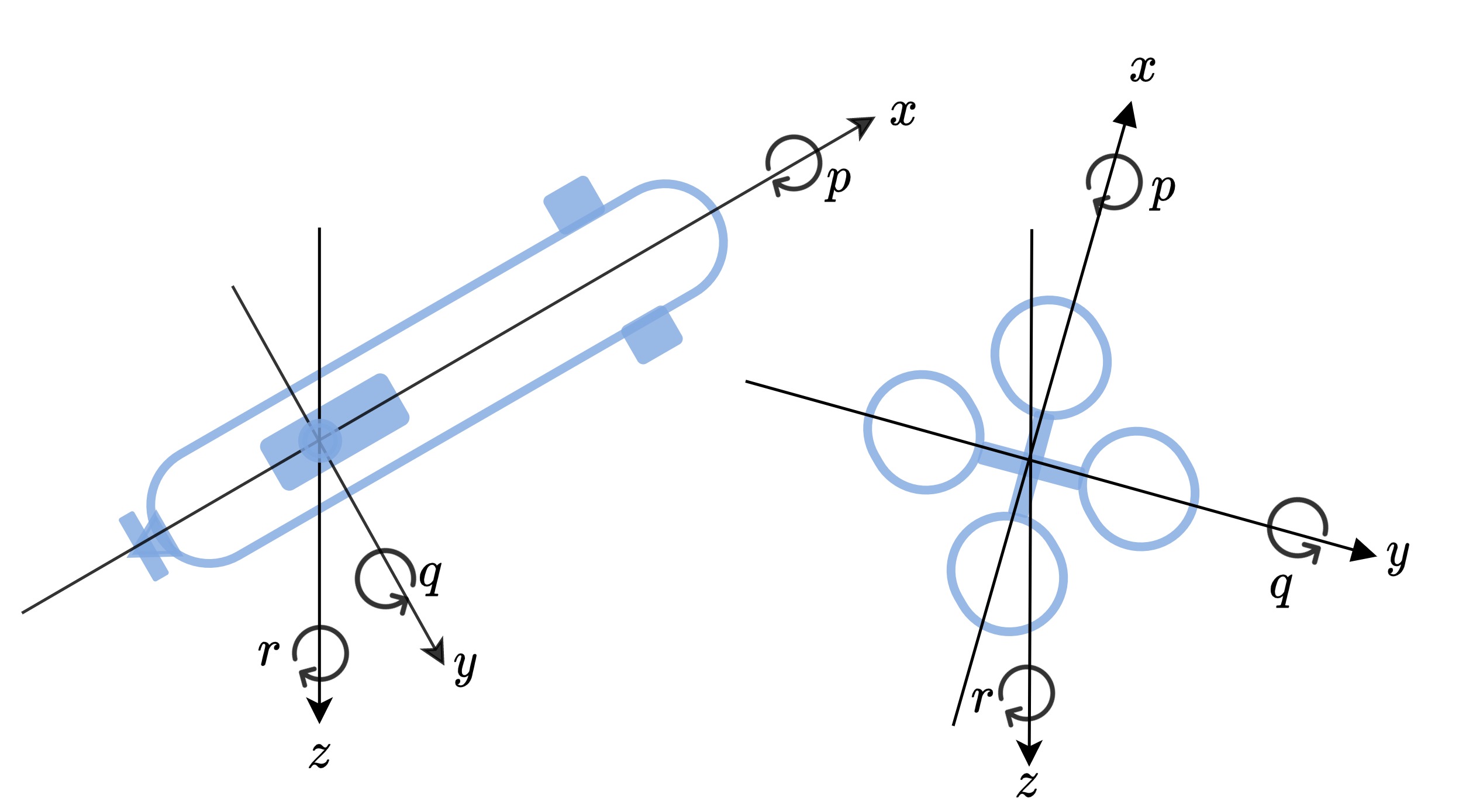
where is the position vector error states expressed in the navigation frame, is the velocity vector error states expressed in the navigation frame, is the misalignment vector state expressed in the navigation frame, is the accelerometer bias residuals vector state expressed in the body frame, and is the gyro bias residuals vector state expressed in the body frame. The navigation frame is denoted by and the body frame is denoted by . The navigation frame center is located at the body center of mass, where the -axis points to the geodetic north, -axis points down parallel to local vertical, and -axis completes a right-handed orthogonal frame. The body frame center is located at the center of mass, -axis is parallel to the longitudinal axis of symmetry of the vehicle pointing forwards, the -axis points right, and the -axis points down such that it forms a right-handed orthogonal frame. The linearized, error-state, continuous-time model is
| (2) |
where is the system matrix, is the shaping matrix, and is the system noise vector consisting of the accelerometer, gyro, and their biases random walk noises, respectively [8]. The system matrix, , is given by
| (3) |
where is the transformation matrix between body and navigation frame and can be found explicitly in the literature (see [1, 31, 32]). The shaping matrix is given by
| (4) |
where is an identity matrix.
The corresponding discrete version of the navigation model (for small step sizes), as given in (2), is
| (5) |
The transition matrix, , is defined by a first order approximation as
| (6) |
where is a time index, is the time step size, is the system matrix (obtained using with the estimated state vector at time ), and is a zero mean white Gaussian noise vector. The discretized process noise is given by
| (7) |
where is defined in (using the current estimated state vector at time ), and is the continuous process noise matrix.
The discrete es-EKF, as described here, is used in the fusion process between the INS and the external measurements. Equations summarize the navigation filter equations[1, 31]:
| (8) |
| (9) |
| (10) |
| (11) |
| (12) |
where is the prior estimate of the error state and is the posterior estimate, with their corresponding covariance matrices and , respectively, is the Kalman gain, is the measurement residual, is the measurement matrix, and is the measurement noise covariance matrix, assumed known and constant.
II-A Measurement Model
The GNSS position measurements are available in a constant and lower frequency then that of the IMU. After processing, the GNSS receiver outputs the vehicle position vector in the navigation frame, where it is used as an update in the navigation filter. Hence, the corresponding time-invariant GNSS measurement matrix is given by
| (13) |
The corresponding measurement residual is given by
| (14) |
where is an additive, discretized, zero mean white Gaussian noise. It is assumed that and are uncorrelated.
II-B Model Based-Adaptive Noise Covariance
The es-EKF minimizes the tracking error without changing matrix online; that is, the process noise covariance is constant throughout the operation. As shown in the literature, [17] and the references therein, tuning online greatly improves the navigation filter performance.
For simplicity, we assume is a diagonal matrix, thus no correlation exists between the noise terms.
The optimal diagonal matrix at time step is defined by
| (15) |
where is the admissible set of at time index , is the ground truth (GT) state at time index , and is the second Euclidean norm.
The most common approach to estimate in an adaptive es-EKF framework was suggested in [16, 17], and is based on the innovation matrix for a window of size :
| (16) |
where is the innovation matrix and the innovation vector is defined by
| (17) |
The innovation matrix, (16), is used together with the Kalman gain, , to adapt , as follows:
| (18) |
III A Hybrid Adaptive Navigation Filter
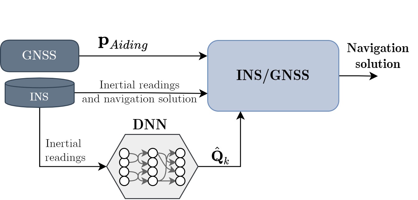
We rely on the well established, model-based es-EKF, yet instead of a model-based adaptive approach, a data-driven approach is used to regress the momentary process noise covariance, and, as a result, creates a hybrid adaptive es-EKF. To this end, the navigation filter equations (8)-(12) are used, but instead of using a constant process noise (7) or a model-based adaptive process noise (18), we derive a data-driven approach to estimate the time-varying continuous process noise covariance matrix . Our proposed hybrid adaptive es-EKF framework, suitable for any aided INS scenario, is presented in Fig. 1.
III-A Data-Driven Based Adaptive Noise Covariance
It is assumed that the continuous process noise covariance matrix, , at time , is a diagonal matrix with the following structure:
| (19) |
where the variance for each of the accelerometer axes is given by and for the gyroscope by (). The biases are modeled by random walk processes, and their variances are set to . By taking this approach, our goal is to ease a machine learning (ML) algorithm for accurately regressing the six unknown variances in (19) and thereby claim that these are the dominant variances needed in an adaptive framework.
We define a general one-dimensional series of length of the inertial sensor (accelerometer or gyroscope) readings in a single axis by
| (20) |
The discussed optimization problem is to find such that the position error is minimized. By doing that for all six IMU channels, the es-EKF considers an optimal system noise covariance matrix and provides improved tracking performance. The power of ML increases the ability to solve many difficult and non-conventional tasks. To determine in (15), the problem is formulated as a SL problem. Formally, we search for a model to relate an instance space, , and a label space, . We assume that there exists a target function, , such that .
Thus, the SL task for adaptive determination of the process noise covariance is to find , given a finite set of labeled examples, inertial sensor readings, and corresponding process noise variance values:
| (21) |
The SL approach aims to find a function that best estimates . To that end, for the training process, a loss function, , is defined to quantify the quality of with respect to . The loss function is given by
| (22) |
where is the number of examples, and is the example index. Minimizing in a training/test procedure leads to the target function. In our problem, the loss function is given by
| (23) |
where is the estimated term obtained by the learning model during the training process.
In this work, the train dataset used to find the function given the labeled examples (21), as described in the next section.
III-B Dataset Generation
There are several existing inertial datasets as were recently summarized in [33]. Yet, none of those datasets fits our problem as they do not provide enough IMU readings with different noise characteristics. As a consequence, we generated are own dataset using a simulation (detailed in Appendix -B).
To generate the dataset six different baseline trajectories were simulated as presented in Fig. 2(a) and in Fig. 3. The richness of the trajectories, as a result of their diversity, allows the establishment of a model to cope with unseen trajectories. Each baseline trajectory was created by generating ideal IMU readings for a period of s in a sampling rate of Hz, resulting in a sequence of samples for each baseline trajectory as shown in Fig. 2.
Our task is to estimate the system noise covariance matrix, or specifically the noise variance of each IMU channel. Hence, we divided each of the six IMU channels and corrupted their perfect data with additive white Gaussian noise with variance in the range of , with 15 different values inside this interval, as shown in Fig. 2(b).
Hence, each baseline trajectory has series of noisy inertial samples, as shown in Fig. 2(b). The justification to include a simple noise model lies in the momentary IMU measurement noise covariance sequence. A short time window for the IMU measurements is considered and allows characterizing the noise with its variance only. Next, the series length is chosen, and a corresponding labeled database is generated as shown in Fig. 2(c). Lastly, we choose samples and create batches corresponding to two seconds each with a total of . Then, these batches are randomly divided into train and test datasets in such a manner that all baseline trajectories are included in the train and the test sets in a ratio of 80:20, as described in Fig. 2(d).
III-C Architecture design
Several architectures were designed and evaluated. They included a recurrent DNN, and, in particular, the long short-term memory (LSTM) architectures for time series data. However, in our problem they did not perform well and failed in generalization of the noise variance property. One of the architecture we examined included a bi-directional LSTM layer followed by two linear layers. The training failed as the temporal information wasn’t relevant for this task. On the other hand, an architecture with only convolution layers achieved satisfactory results, where it minimized the test loss very fast and obtained a low position root mean squared error (PRMSE) (the metric is defined in (25)). This result is due to the spatial information the noisy IMU signals have, allowing to capture the dynamics and statistical properties of the measurements. This information structure was easily captured by the spatial convolutional operates in the convolution layers. As the goal of this paper is to lay the foundations for a hybrid adaptive navigation filter approach, we describe here only the DNN architecture as presented in Fig. 4. Our DNN model has the following layers:
-
1.
Linear layer: This is the simplified layer structure that applies a linear transformation to the incoming data from the previous layer. The input features are received in the form of a flattened 1D vector and are multiplied by the weighting matrix.
-
2.
Conv1D layer: A convolutional, one-dimensional (Conv1D) layer creates a convolution kernel that is convolved with the layer input over a single spatial dimension to produce a vector of outputs. During the training phase the DNN learns the optimal weights of the kernels. In our DNN model the input layer is followed by a chain of three Conv1D layers. There are five kernels for the first layer and three kernels for the second and third layers. The kernel size decreases as the inputs go deep: the first Conv1D layer has twenty kernels, the second Conv1D layer has ten kernels, and the third Conv1D layer has five kernels.
-
3.
Global average pooling layer: Pooling layers help with better generalization capability as they perform down sampling feature map. In this way, the robustness of the DNN grows. For example, better handling with changes in the position of the features inside the 1D input vector. For the DNN architecture we selected the global average pooling method, which calculates the average for each input channel and flattens the data so it passes from Conv1D through the linear layers.
-
4.
Leaky ReLU: Leaky rectified linear unit [34] is a nonlinear activation function obtaining a value with the following output:
(24) The main advantage of the leaky ReLU over the classical ReLU (0 for ) is the small positive gradient when the unit is not active, which deals better with the dying ReLU problem [35]. The leaky ReLU functions were combined after each layer in the DNN model.
-
5.
Layer normalization: One of the challenges of DNN is that the gradients with respect to the weights in one layer are highly dependent on the outputs of the neurons in the previous layer, especially if these outputs change in a highly correlated way [36]. Batch normalization, and in particular layer normalization, was proposed to reduce such an undesirable covariate shift. The layer normalization was added after every Conv1D layer (together with the leaky ReLU layer).
The parameters of the above layers are as follow: a series of samples is inserted to a one-dimensional convolutional layer (Conv1D) with a kernel size equals to with five filters. Then, a leaky ReLU activation function and normalization layer are applied, adding nonlinearity for better generalization capability of the DNN. We duplicated this structure twice more with three filters each and smaller kernels: the second with a kernel size equals to ten and the third with a kernel size equals to five. The output is inserted to a global average pooling layer followed by four linear layers, with leaky ReLU activation functions between them, with and weights, retrospectively. Finally, the DNN outputs the process noise variance.
III-D Hybrid Learning Approach
In this work, GNSS position updates are employed to aid the INS and demonstrate our hybrid learning approach. Applying the suggested adaptive tuning approach in online setting involves integrating the INS/GNSS with the regressor as presented in Fig. 5. Algorithm 1 describes the INS/GNSS with process noise covariance learning in a real time setup. The IMU signals are inserted both into the INS/GNSS filter and the DNN model. The regressed continuous process noise covariance is plugged into to obtain the discrete one, which in turn is substituted into .
IV Analysis and Results
We employ the following two metrics to evaluate the position accuracy of the proposed approach:
-
•
Position root mean squared error ( norm) for all three axes:
(25) -
•
Position mean absolute error for all six IMU channels:
(26)
where is the number of samples, is a running index for the samples, is the running index for the Cartesian coordinate system, and is the position error term.
IV-A Train Dataset Analysis
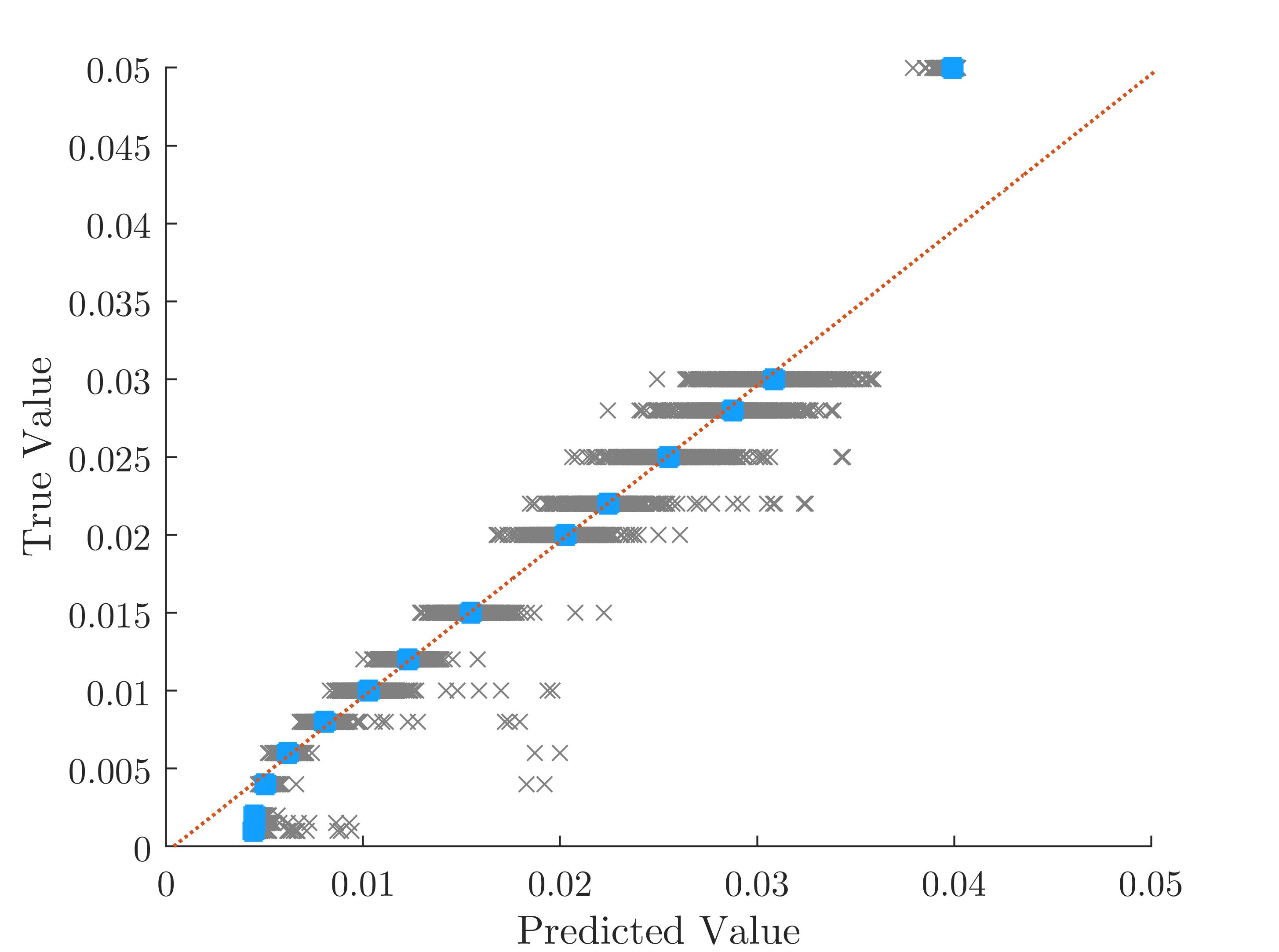
The proposed DNN architecture, presented in Section III-C, was trained on the dataset described in Section III-B. After epochs it achieved an RMSE of on the test set, showing the proposed DNN generalization capability and thereby establishing the trained DNN regressor model. The training process was done in mini-batches of examples each. The ADAM optimizer [37] was used with an initial learning rate of and a learn-rate-schedule with a drop factor of after epochs. In our working environment (Intel i7-6700HQ [email protected] 16GB RAM with MATLAB), the training time for input length of 200 samples elapsed about three hours. The averaged inference time is . Fig. 6 presents the performance for samples where the red line is the desired one, representing when the GT value is equal to the DNN predicted value. The gray points represent the performance of the test set with the trained DNN model. The mean values of the test set lies near the red line (blue points) for most cases.
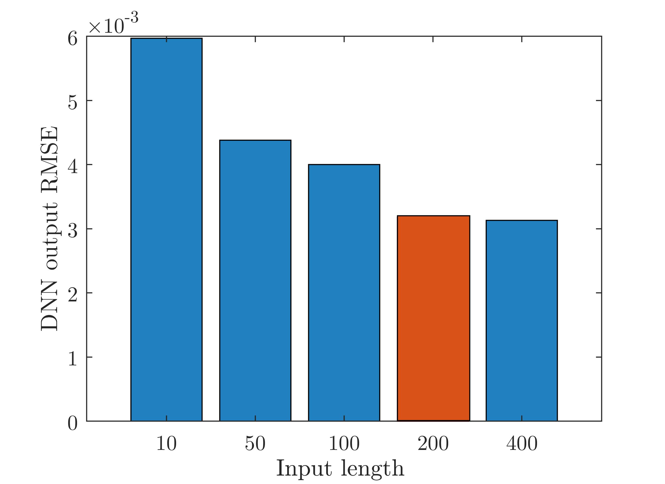
The INS/GNSS fusion is mostly performed under real-time conditions, where latency in the position computation might degrade the performance. Thus, the influence of the IMU sequence length input was examined. The system noise covariance matrix was learned, based on series of length . As , the probability of learning the correct terms grows, since the DNN can capture the signal intrinsic properties easier using more data; however, the latency grows. Considering this trade-off, we trained the chosen architecture with various values and calculated the RMSE as shown in Fig. 7. As expected, obtained the minimum RMSE, yet for the rest of the analysis we chose (similar RMSE) to receive the regression result as it is given in a shorter time period. For example, in the stimulative train and test dataset the sampling rate is Hz, thus working with gives the regression result every two seconds instead of working with four seconds ().
IV-B Field experiment
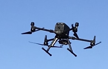
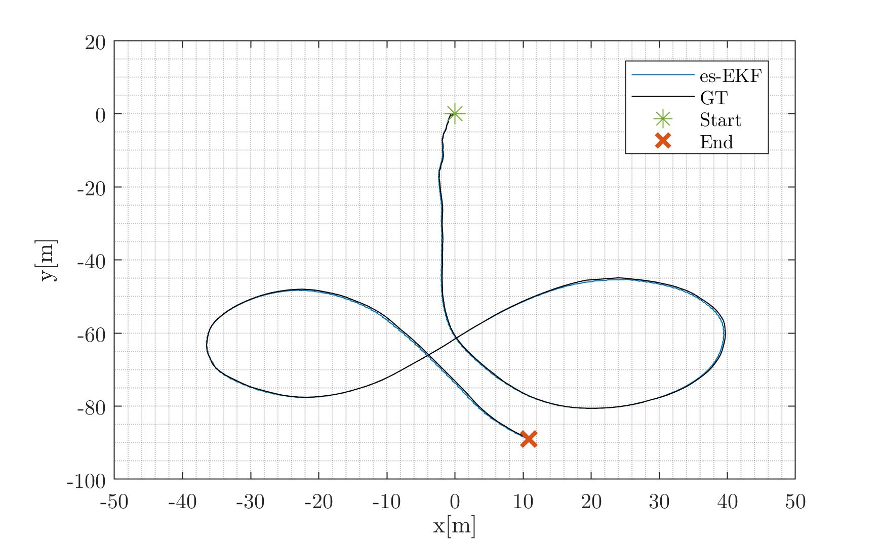
A field experiment with the DJI Matrice 300 [38] was performed (Fig. 8). The trajectory is shown in Fig. 9. A figure-eight trajectory was made with some additional approximated straight line segments. The experiment parameters, including the GNSS RTK GT values and IMU, are given in Table I. The quadrotor dataset was published in [39] and is publicly available at https://github.com/ansfl/Navigation-Data-Project.
| Description | Symbol | Value |
|---|---|---|
| GNSS noise (var) - horizon | ||
| GNSS noise (var) - vertical | ||
| GNSS step size | ||
| IMU step size | ||
| Accelerometer noise (MPU-9250) | ||
| Gyroscope rate noise (MPU-9250) | ||
| Experiment duration | ||
| Initial velocity | ||
| Initial position |
Equations (2)-(12) were used as a model-based es-EKF with a constant process noise covariance matrix. Three different cases of the model-based es-EKF with constant process noise covariance matrix (MB-EKF-CQ) were examined:
-
•
MB-EKF-CQ1: .
-
•
MB-EKF-CQ2: .
-
•
MB-EKF-CQ3: .
In addition, using (16)-(18), three different (window size length) cases of model-based es-EKF with the adaptive process noise covariance matrix (MB-EKF-AQ) were examined:
-
•
MB-EKF-AQ1: .
-
•
MB-EKF-AQ2: .
-
•
MB-EKF-AQ3: .
All six approaches were compared to our proposed hybrid adaptive EKF (HB-AEKF) using the trained network, as described in the previous section. Results in terms of PMAE and PRMSE are presented in Table 2. The MB-EKF-AQ model-based adaptive filters obtained better performance than the MB-EKF-CQ constant process noise filters. In particular, MB-EKF-CQ3 achieved the best performance for constant process noise with a PMAE of and a PRMSE of , where MB-EKF-AQ3 manged to improve them by and , respectively. Our proposed hybrid adaptive approach, HB-AEKF, with an input length of samples, obtained the best performance, with PMAE and PRMSE improving MB-EKF-AQ3 by and , respectively.
The parameters time evaluation were obtained using our HB-AEKF approach—are shown in Fig. 10 for both accelerometers and gyroscopes. Their behavior shows fluctuations in the first seconds and then steady-state behavior. This behavior can be attributed to the convergence of the es-EKF - once it obtains enough data and captures the IMU noise statistic.
| HB-AEKF (ours) | ||
|---|---|---|
| MB-EKF-AQ1 | ||
| MB-EKF-AQ2 | ||
| MB-EKF-AQ3 | ||
| MB-EKF-CQ1 | ||
| MB-EKF-CQ2 | ||
| MB-EKF-CQ3 |
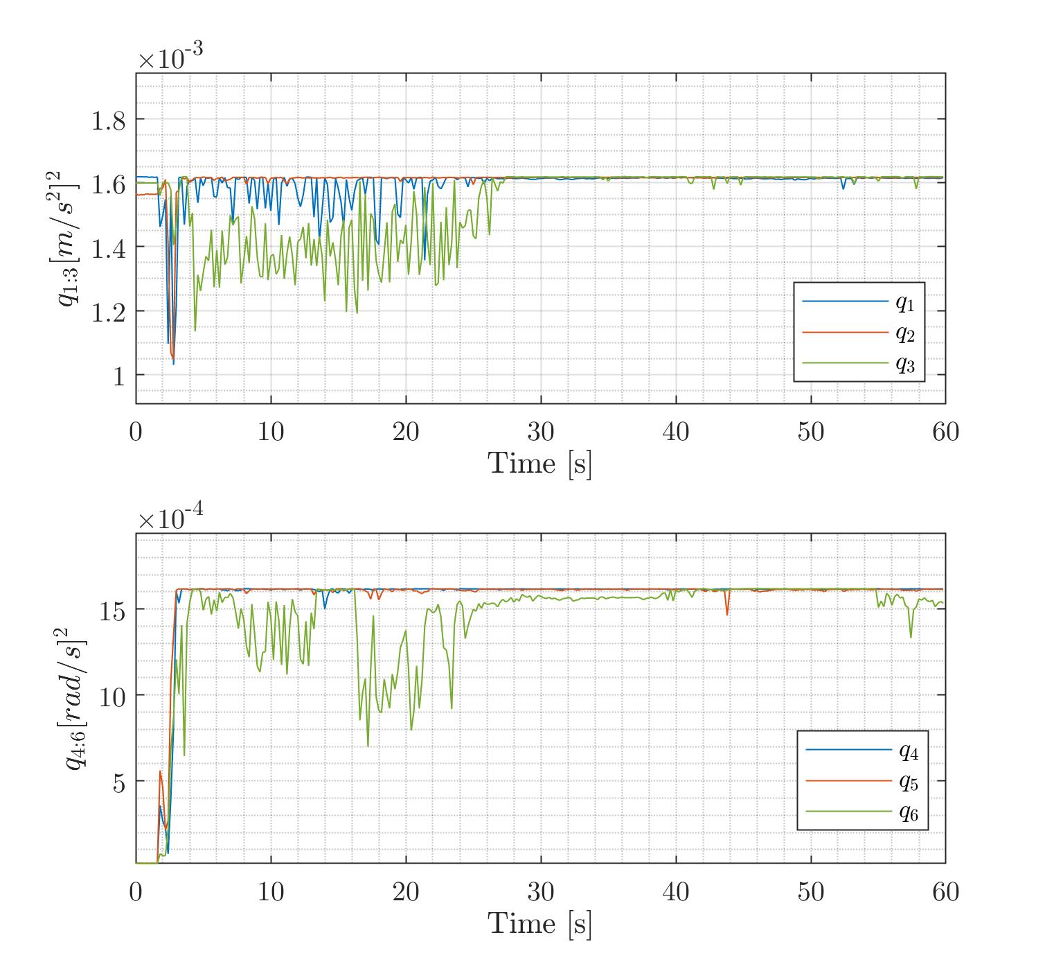
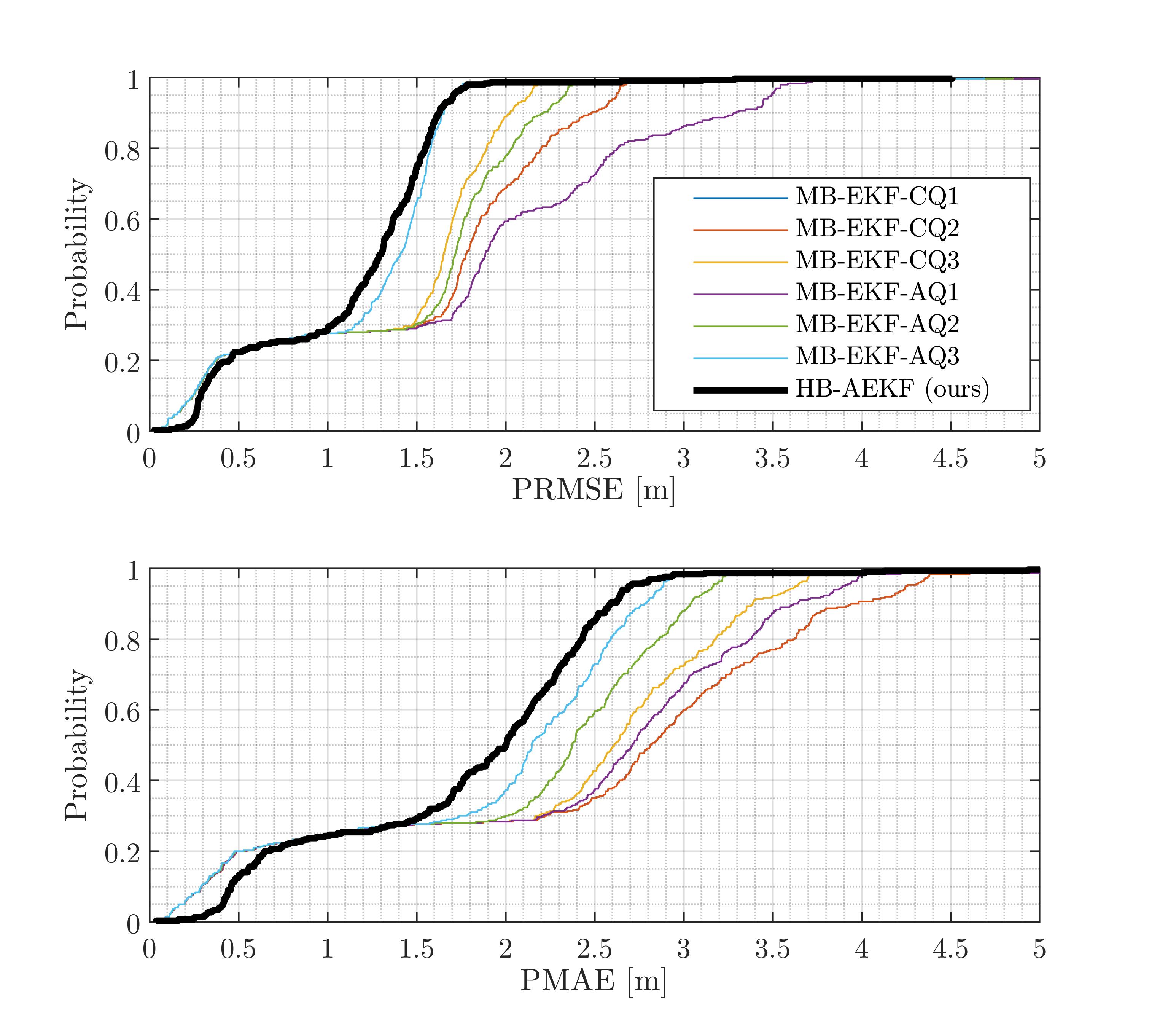
Fig. 11 summarizes the positioning performance by providing two graphs of the cumulative density function (CDF); one representing PRMSE and the other the PMAE. In those plots, all three MB-EKF-AQ and three MB-EKF-CQ approaches are presented as well as our proposed HB-AEKF hybrid approach (black lines). Both graphs show clearly that the entire error is lower for HB-AEKF than all other approaches. The PRMSE of the MB-AEKF is lower than and the PMAE lower than for the entire scenario. In comparison with the MB-EKF-AQ1 approach, the maximum PRMSE and the maximum PMAE might grow too much: and , respectively.
V Conclusions
The proper choice for the system noise covariance matrix is critical for accurate INS/GNSS fusion. In this paper, a hybrid learning and model based approach was suggested in an adaptive filter framework. To that end, a novel DNN-based approach to learn and online tune the system noise covariance was developed. The input to the DNN is only the IMU readings. This learning approach was then combined with the model based es-EKF, resulting in a hybrid adaptive filter.
The DNN model has been trained only once on a simulated database consisting of six different baseline trajectories. Analysis on this dataset showed a trade-off between accuracy and the regression solution latency, where as the latency increases the accuracy decreases. Relying on this analysis, an input length of samples was chosen.
To validate the performance of the proposed approach, it was compared to six model-based approaches representing both constant and adaptive process noise covariance selection. Quadrotor field experiments were conducted and used as an additional test dataset on the trained network. We obtained state-of-the-art results for each noise value compared to classical adaptive KF approaches; a PRMSE lower than and a PMAE lower than were obtained using our suggested approach, compared to a PRMSE of and a PMAE of a that were obtained using the innovation-based adaptive approach and classical tuning. Results in a total PRMSE improvement of and PMAE improvement of .
This improvement also demonstrates the robustness and generalization properties of the proposed DNN architecture, enabling it to cope with unseen data from different IMU sensors. In addition, and together with the train dataset results, it proves our hypothesis of regressing only the first six elements in the diagonal of the continuous process noise covariance matrix.
Although demonstrated for quadrotor INS/GNSS fusion, the proposed approach can be elaborated for any external sensor aiding the INS and for any type of platform.
Although the present study demonstrated a small improvement over model-based methods using the test dataset of a quadrotor INS/GNSS fusion, it introduces a hybrid framework to combine deep learning in an adaptive navigation filter. This approach can be applied to other platforms, dynamics and external sensor aiding the INS and serve as a foundation approach for future work in the field.
-A Abbreviations
| Abbreviation | Description |
|---|---|
| AUV | autonomous underwater vehicle |
| CDF | cumulative density function |
| Conv1D | one-dimensional convolution |
| DNN | deep neural network |
| DVL | Doppler velocity log |
| EKF | extended Kalman filter |
| es | error state |
| GNSS | global navigation satellite system |
| GT | ground truth |
| HB-AEKF | hybrid based adaptive EKF |
| INS | inertial navigation system |
| LSTM | long short-term memory |
| MB-EKF-AQ | model based EKF adaptive Q |
| MB-EKF-CQ | model based EKF constant Q |
| ML | machine learning |
| NED | North-East-Down |
| PDR | pedestrian dead-reckoning |
| PMAE | position mean absolute error |
| PRMSE | position RMSE |
| RMSE | root mean squared error |
| SL | supervised learning |
| UAV | unmanned air vehicles |
-B Dataset Generation
-B1 INS Equations of Motion
The INS equations of motion include the rate of change of the position, velocity, and the transformation between the navigation and body frame, as shown in Fig.12.
The position vector is given by
| (27) |
where is the latitude, is the longitude, and is the altitude. The velocity vector is Earth referenced and expressed in the North-East-Down (NED) coordinate system:
| (28) |
where denote the velocity vector components in north, east, and down directions, respectively. The rate of change of the position is given by [1]
| (29) |
where and are the meridian radius and the normal radius of curvature, respectively. The rate of change of the velocity vector is given by [1]
| (30) |
where is the transformation matrix from body frame to the navigation frame. is the accelerometers vector state expressed in the body frame, is the gravity vector expressed in the navigation frame. is the angular velocity vector between the earth centered earth fixed (ECEF) frame and the navigation frame. The angular velocity vector between ECEF and the inertial frame is given by and the rate of change of the transformation matrix is given by [1]
| (31) |
where is the angular velocity vector as obtained by the gyroscope and is the angular velocity vector between the navigation frame and the inertial frame expressed in the body frame. The angular velocity between the navigation frame and the inertial frame expressed in the navigation frame is given by . The alignment between body frame and navigation frame can be obtained from , as follows
| (32) |
where is the roll angle, is the pitch angle, and is the yaw angle. These three angles are called Euler angles.
-B2 IMU readings
The GT trajectories were created by tuning vehicle angular rates, , and vehicle accelerations, , as follows [40]
| (33) |
and,
| (34) |
The transformation between the desired motion and the INS framework for the gyroscope readings is given by [40]
| (35) |
where
| (36) |
and from (30) the accelerometer readings are
| (37) |
Once, the GT IMU readings (35) and (37) are obtained, noise characteristics as described in Section III are added to create our dataset.
References
- [1] J. Farrell, Aided navigation: GPS with high rate sensors. McGraw-Hill, Inc., 2008, pp: 393-395.
- [2] D. Wang, Y. Dong, Z. Li, Q. Li, and J. Wu, “Constrained mems-based gnss/ins tightly coupled system with robust kalman filter for accurate land vehicular navigation,” IEEE Transactions on Instrumentation and Measurement, vol. 69, no. 7, pp. 5138–5148, 2019.
- [3] G. Wang, X. Xu, J. Wang, and Y. Zhu, “An enhanced ins/gnss tightly coupled navigation system using time-differenced carrier phase measurement,” IEEE Transactions on Instrumentation and Measurement, vol. 69, no. 7, pp. 5208–5218, 2019.
- [4] L. Paull, S. Saeedi, M. Seto, and H. Li, “AUV navigation and localization: A review,” IEEE Journal of Oceanic Engineering, vol. 39, no. 1, pp. 131–149, 2013.
- [5] S. Gupte, P. I. T. Mohandas, and J. M. Conrad, “A survey of quadrotor unmanned aerial vehicles,” in 2012 Proceedings of IEEE Southeastcon. IEEE, 2012, pp. 1–6.
- [6] Q. Xu, X. Li, and C.-Y. Chan, “Enhancing localization accuracy of mems-ins/gps/in-vehicle sensors integration during gps outages,” IEEE Transactions on Instrumentation and Measurement, vol. 67, no. 8, pp. 1966–1978, 2018.
- [7] Y. Cui, S. Liu, J. Yao, and C. Gu, “Integrated positioning system of unmanned automatic vehicle in coal mines,” IEEE Transactions on Instrumentation and Measurement, vol. 70, pp. 1–13, 2021.
- [8] Y. Bar-Shalom, X. R. Li, and T. Kirubarajan, Estimation with applications to tracking and navigation: theory algorithms and software. John Wiley & Sons, 2004.
- [9] X. Lyu, B. Hu, K. Li, and L. Chang, “An adaptive and robust UKF approach based on Gaussian process regression-aided variational Bayesian,” IEEE Sensors Journal, vol. 21, no. 7, pp. 9500–9514, 2021.
- [10] C. H. Kang, C. G. Park, and J. W. Song, “An adaptive complementary kalman filter using fuzzy logic for a hybrid head tracker system,” IEEE Transactions on Instrumentation and Measurement, vol. 65, no. 9, pp. 2163–2173, 2016.
- [11] N. Davari and A. Gholami, “An asynchronous adaptive direct Kalman filter algorithm to improve underwater navigation system performance,” IEEE Sensors Journal, vol. 17, no. 4, pp. 1061–1068, 2016.
- [12] D.-J. Jwo and S.-H. Wang, “Adaptive fuzzy strong tracking extended Kalman filtering for gps navigation,” IEEE Sensors Journal, vol. 7, no. 5, pp. 778–789, 2007.
- [13] M. A. K. Jaradat and M. F. Abdel-Hafez, “Enhanced, delay dependent, intelligent fusion for INS/GPS navigation system,” IEEE Sensors Journal, vol. 14, no. 5, pp. 1545–1554, 2014.
- [14] X. Tong, Z. Li, G. Han, N. Liu, Y. Su, J. Ning, and F. Yang, “Adaptive ekf based on hmm recognizer for attitude estimation using mems marg sensors,” IEEE Sensors Journal, vol. 18, no. 8, pp. 3299–3310, 2017.
- [15] J. He, C. Sun, B. Zhang, and P. Wang, “Adaptive error-state kalman filter for attitude determination on a moving platform,” IEEE Transactions on Instrumentation and Measurement, vol. 70, pp. 1–10, 2021.
- [16] R. Mehra, “On the identification of variances and adaptive Kalman filtering,” IEEE Transactions on Automatic Control, vol. 15, no. 2, pp. 175–184, 1970.
- [17] L. Zhang, D. Sidoti, A. Bienkowski, K. R. Pattipati, Y. Bar-Shalom, and D. L. Kleinman, “On the identification of noise covariances and adaptive Kalman filtering: A new look at a 50 year-old problem,” IEEE Access, vol. 8, pp. 59 362–59 388, 2020.
- [18] H. Yan, Q. Shan, and Y. Furukawa, “RIDI: Robust IMU double integration,” in Proceedings of the European Conference on Computer Vision (ECCV), 2018, pp. 621–636.
- [19] S. Herath, H. Yan, and Y. Furukawa, “Ronin: Robust neural inertial navigation in the wild: Benchmark, evaluations, & new methods,” in 2020 IEEE International Conference on Robotics and Automation (ICRA). IEEE, 2020, pp. 3146–3152.
- [20] O. Asraf, F. Shama, and I. Klein, “Pdrnet: A deep-learning pedestrian dead reckoning framework,” IEEE Sensors Journal, 2021.
- [21] A. Manos, T. Hazan, and I. Klein, “Walking direction estimation using smartphone sensors: a deep network-based framework,” IEEE Transactions on Instrumentation and Measurement, 2022.
- [22] C. Chen, P. Zhao, C. X. Lu, W. Wang, A. Markham, and N. Trigoni, “Deep-learning-based pedestrian inertial navigation: Methods, data set, and on-device inference,” IEEE Internet of Things Journal, vol. 7, no. 5, pp. 4431–4441, 2020.
- [23] M. Yona and I. Klein, “Compensating for partial doppler velocity log outages by using deep-learning approaches,” in 2021 IEEE International Symposium on Robotic and Sensors Environments (ROSE). IEEE, 2021, pp. 1–5.
- [24] D. Li, J. Xu, H. He, and M. Wu, “An underwater integrated navigation algorithm to deal with dvl malfunctions based on deep learning,” IEEE Access, vol. 9, pp. 82 010–82 020, 2021.
- [25] M. Brossard and S. Bonnabel, “Learning wheel odometry and imu errors for localization,” in 2019 International Conference on Robotics and Automation (ICRA). IEEE, 2019, pp. 291–297.
- [26] A. Shurin and I. Klein, “Quadnet: A hybrid framework for quadrotor dead reckoning,” Sensors, vol. 22, no. 4, p. 1426, 2022.
- [27] C. Shen, Y. Zhang, X. Guo, X. Chen, H. Cao, J. Tang, J. Li, and J. Liu, “Seamless gps/inertial navigation system based on self-learning square-root cubature kalman filter,” IEEE Transactions on Industrial Electronics, vol. 68, no. 1, pp. 499–508, 2020.
- [28] B. Or and I. Klein, “Learning vehicle trajectory uncertainty,” arXiv preprint arXiv:2206.04409, 2022.
- [29] J. Liu and G. Guo, “Vehicle localization during gps outages with extended kalman filter and deep learning,” IEEE Transactions on Instrumentation and Measurement, vol. 70, pp. 1–10, 2021.
- [30] M. Brossard, S. Bonnabel, and A. Barrau, “Denoising imu gyroscopes with deep learning for open-loop attitude estimation,” IEEE Robotics and Automation Letters, vol. 5, no. 3, pp. 4796–4803, 2020.
- [31] P. D. Groves, Principles of GNSS, Inertial, and Multisensor Integrated Navigation Systems 2nd ed. Boston, MA: Artech House, 2013.
- [32] R. G. Brown and P. Y. Hwang, Introduction to random signals and applied Kalman filtering. Wiley New York, Third Edtion, 1992.
- [33] A. Shurin, A. Saraev, M. Yona, Y. Gutnik, S. Faber, A. Etzion, and I. Klein, “The autonomous platforms inertial dataset (table 1),” IEEE Access, vol. 10, pp. 10 191–10 201, 2022.
- [34] A. L. Maas, A. Y. Hannun, A. Y. Ng et al., “Rectifier nonlinearities improve neural network acoustic models,” in Proc. icml, vol. 30, no. 1. Citeseer, 2013, p. 3.
- [35] L. Lu, Y. Shin, Y. Su, and G. E. Karniadakis, “Dying relu and initialization: Theory and numerical examples,” arXiv preprint arXiv:1903.06733, 2019.
- [36] J. L. Ba, J. R. Kiros, and G. E. Hinton, “Layer normalization,” arXiv preprint arXiv:1607.06450, 2016.
- [37] D. P. Kingma and J. Ba, “Adam: A method for stochastic optimization,” arXiv preprint arXiv:1412.6980, 2014.
- [38] DJI, “Matrice 300 RTK, Aircraft Specifications,” Website source: https://www.dji.com/matrice-300/specs, 2021.
- [39] A. Shurin, A. Saraev, M. Yona, Y. Gutnik, S. Faber, A. Etzion, and I. Klein, “The autonomous platforms inertial dataset,” IEEE Access, vol. 10, pp. 10 191–10 201, 2022.
- [40] D.-J. Jwo, J.-H. Shih, C.-S. Hsu, and K.-L. Yu, “Development of a strapdown inertial navigation system simulation platform,” Journal of Marine Science and Technology, vol. 22, no. 3, pp. 381–391, 2014.
![[Uncaptioned image]](https://cdn.awesomepapers.org/papers/ac619d3a-d30f-497d-90f1-c2900d7b648e/Barak.jpeg) |
Barak Or (Member, IEEE) received a B.Sc. degree in aerospace engineering from the Technion–Israel Institute of Technology, Haifa, Israel, a B.A. degree (cum laude) in economics and management, and an M.Sc. degree in aerospace engineering from the Technion–Israel Institute of Technology in 2016 and 2018. He is currently pursuing a Ph.D. degree with the University of Haifa, Haifa.
His research interests include navigation, deep learning, sensor fusion, and estimation theory. |
![[Uncaptioned image]](https://cdn.awesomepapers.org/papers/ac619d3a-d30f-497d-90f1-c2900d7b648e/klein.jpg) |
Itzik Klein (Senior Member IEEE) received B.Sc. and M.Sc. degrees in Aerospace Engineering from the Technion-Israel Institute of Technology, Haifa, Israel in 2004 and 2007, and a Ph.D. degree in Geo-information Engineering from the Technion-Israel Institute of Technology, in 2011. He is currently an Assistant Professor, heading the Autonomous Navigation and Sensor Fusion Lab, at the Hatter Department of Marine Technologies, University of Haifa. His research interests include data driven based navigation, novel inertial navigation architectures, autonomous underwater vehicles, sensor fusion, and estimation theory. |