A High Angular Resolution Survey of Massive Stars in Cygnus OB2:
Adaptive Optics Results from the
Gemini Near-InfraRed Imager
Abstract
We present results of a high angular resolution survey of massive OB stars in the Cygnus OB2 association that we conducted with the NIRI camera and ALTAIR adaptive optics system of the Gemini North telescope. We observed 74 O- and early B-type stars in Cyg OB2 in the infrared bands in order to detect binary and multiple companions. The observations are sensitive to equal-brightness pairs at separations as small as , and progressively fainter companions are detectable out to mag at a separation of . This faint contrast limit due to readnoise continues out to 10 arcsec near the edge of the detector. We assigned a simple probability of chance alignment to each companion based upon its separation and magnitude difference from the central target star and upon areal star counts for the general star field of Cyg OB2. Companion stars with a field membership probability of less than are assumed to be physical companions. This assessment indicates that of the targets have at least one resolved companion that is probably gravitationally bound. Including known spectroscopic binaries, our sample includes 27 binary, 12 triple, and 9 systems with four or more components. These results confirm studies of high mass stars in other environments that find that massive stars are born with a high multiplicity fraction. The results are important for the placement of the stars in the H-R diagram, the interpretation of their spectroscopic analyses, and for future mass determinations through measurement of orbital motion.
, , , , , , , , , , ,
1 Introduction
Massive stars profoundly influence the evolution of the Universe, from galactic dynamics and structure to star formation. They are often found with bound companions. Massive stars have a higher frequency of multiplicity than cooler, less massive stars (Raghavan et al., 2010; Duchêne & Kraus, 2013), especially when they are found in clusters (Mason et al., 2009). Spectroscopic studies of massive stars in the Milky Way (Sana et al., 2012) and in the Tarantula Nebula region of the Large Magellanic Cloud (Sana et al., 2013) demonstrate that perhaps of massive O-type stars have binary companions in orbits small enough that the stars will interact over their lifetime. Our knowledge of O-type multiple systems in larger orbits with periods in the range from years to thousands of years is incomplete due their great distances, but high angular resolution methods are beginning to fill in this period gap (Maíz Apellániz et al., 2019; Le Bouquin et al., 2017; Aldoretta et al., 2015; Sana et al., 2014).
At a distance of 1.33 – 1.7 kpc (Massey & Thompson, 1991; Torres-Dodgen et al., 1991; Hanson, 2003; Rygl et al., 2012; Kiminki et al., 2015), Cygnus OB2 = Cyg OB2 is the second closest OB association (after Ori OB1) that provides us with an example of a nearby, young stellar environment, rich in high-mass stars. Due to uneven extinction towards the region (Wright et al., 2015), the cluster begins to be unveiled in the infrared (IR). Torres-Dodgen et al. (1991) estimate the age of the association to be least 3 Myr through analysis of their Strömgren and infrared photometry, and Wright et al. (2015) argue that star formation has occurred more or less continuously over the last 1 to 7 Myr based upon the positions of the stars in the Hertzsprung - Russell (H-R) diagram. The young nature of the association is further established by the detection of X-rays from young, low mass stars in the region (Albacete Colombo et al., 2007; Wright & Drake, 2009; Wright et al., 2012). Spectroscopic surveys by Massey & Thompson (1991), Hanson (2003), and Kiminki et al. (2007) have established the early-type classifications of these stars. Massive stars are short-lived and therefore spend most of their formative years shrouded in their natal clouds, so that when they shed these clouds and a hot star is revealed, it is usually well into the main sequence stage of its life. The multiplicity of massive stars must play an important role in their formation because so many are members of binary systems (Zinnecker & Yorke, 2007). Massive stars are formed through the turbulent core collapse of a single cloud or by competitive accretion of multiple stellar seeds in a dense cloud (see the review by Rosen et al. 2020), and models of these processes predict a large incidence of binary stars with specific distributions of mass ratio and separation (Peter et al., 2012; Gravity Collaboration et al., 2018). Therefore, by studying the multiplicity properties of massive stars at an early stage we can test the role of companions in formation theories of massive stars.
The Cyg OB2 association is close enough that with modern-day adaptive optics (AO) we are able to resolve relatively close companions. The ALTAIR AO system and the Near-InfraRed Imager and Spectrograph (NIRI) at the Gemini North Observatory provides an effective tool to search for binaries, as was demonstrated by Lafrenière et al. (2014) in a multiplicity study of young stars in the Upper Sco association. With a resolution of and a sensitivity contrast limit of about 10 mag for differential photometry, the ALTAIR AO infrared system can delve into the depths of the association and find faint companions with periods in the range from hundreds to thousands of years. Our results complement the radial velocity survey of Kobulnicky et al. (2014) (and references therein) who searched for short period, spectroscopic systems in Cyg OB2. They determined that of their sample are spectroscopic binaries with periods less than 45 days.
In this paper, we provide measurements of -band relative photometry and positions of candidate companions to our target stars. These results provide the first step in determining the true multiplicity fraction of widely separated systems. In section 2 we describe the observations of the sample in Cygnus OB2. We present the results of the survey in section 3 along with further details of the calibration in appendices for the astrometry (Appendix A) and photometry (Appendix B). We discuss the detection limits and the identification of probable physical companions in section 4. Section 5 presents the multiplicity fraction and companion frequency for the Cyg OB2 sample and compares these to similar results from studies of massive stars in other locations. We summarize the results and their significance in section 6.
2 Observations
We were able to observe 74 of the brightest O- and B-type stars in Cyg OB2 and one misidentified non-member using the infrared ALTAIR AO system (Richardson et al., 1998; Roberts & Singh, 1998a) at the Gemini North Observatory. We provide a list of our targets in Table 2 (given in full in the electronic version) that gives the target name, celestial coordinates (J2000), spectral classification and reference, optical and infrared (IR) magnitudes, and three measures of interstellar reddening. The majority of stars in this study were selected from the optical survey of Massey & Thompson (1991), who presented Johnson and magnitudes for the brighter stars in the sample as well as reddening towards each star. These targets are identified with prefix “MT” by their number assigned by Massey & Thompson (1991). Seventeen of our targets were selected from the infrared surveys by Comerón et al. (2002, 2008), and these are referenced by a prefix “A” or “B” from those papers. These are redder sources that are not readily detected in the optical surveys, but -band and spectral information are available for some of these from Straižys & Laugalys (2008). An “S” designation is given for three stars from the compilation by Schulte (1958), and the final object is given by its Wolf-Rayet catalog number (van der Hucht, 2001). The spectral classifications are taken from a variety of sources, indicated in the notes below the table. The magnitudes reported are from Massey & Thompson (1991) for the MT # stars and from Straižys & Laugalys (2008) for others. The coordinates and infrared photometry are from the Two Micron All Sky Survey (2MASS; Skrutskie et al. 2006). The reddening estimates are discussed in section 4.3 below. After we completed our observations we learned that the object MT 140 is in fact an intermediate mass object that is not a member of Cyg OB2 (Maíz Apellániz et al., 2016). We include our measurements here for completeness, but it is excluded from the multiplicity analysis.
Wright et al. (2015) describe the massive star content of the Cyg OB2 association, and they suggest that the association hosts 52 O-type stars and 3 Wolf-Rayet stars. Our sample includes 56 O-type stars and one Wolf-Rayet star, plus a number of luminous and/or early type B-stars. Thus, our target list should represent an almost complete sample of the most massive stars () in Cyg OB2 (missing the Wolf-Rayet Stars WR 144 and WR 146).
| Star | Schulte # | R.A. | Dec. | Spectral | Class. | |||||||
|---|---|---|---|---|---|---|---|---|---|---|---|---|
| Name | (HH:MM:SS) | (DD:MM:SS) | Classification | Ref. | (mag) | (mag) | (mag) | (mag) | (mag) | (mag) | (mag) | |
| A 11 | (MT 267) | 20:32:31.539 | +41:14:08.22 | O7.5 III-1 | 1 | 7.817 | 7.094 | 6.664 | 1.32 | |||
| A 12 | 20:33:38.219 | +40:41:06.41 | B0 Ia | 3 | 6.904 | 6.170 | 5.745 | 1.40 | ||||
| A 15 | 20:31:36.909 | +40:59:09.25 | O7 Ib(f) | 3 | 7.913 | 7.208 | 6.811 | 1.32 | ||||
| A 18 | 20:30:07.879 | +41:23:50.47 | O8 V | 3 | 9.397 | 8.739 | 8.365 | 1.25 | ||||
| A 20 | 20:33:02.920 | +40:47:25.45 | O8 II((f)) | 5 | 7.251 | 6.632 | 6.274 | 1.16 | ||||
| A 23 | 20:30:39.710 | +41:08:48.98 | B0.7 | 5 | 6.928 | 6.328 | 5.980 | 1.08 | ||||
| A 24 | 20:34:44.110 | +40:51:58.51 | O6.5 III((f)) | 3 | 8.405 | 7.796 | 7.448 | 1.15 | ||||
| A 25 | 20:32:38.441 | +40:40:44.54 | O8 III | 3 | 8.347 | 7.705 | 7.383 | 1.19 | ||||
| A 26 | 20:30:57.730 | +41:09:57.57 | O9.5 V | 3 | 9.093 | 8.514 | 8.198 | 1.14 | ||||
| A 27 | 20:34:44.719 | +40:51:46.56 | B0 Ia | 3 | 6.683 | 6.062 | 5.731 | 1.14 | ||||
| A 29 | 20:34:56.061 | +40:38:18.06 | O9.7 Iab | 5 | 7.440 | 6.859 | 6.545 | 1.05 | ||||
| A 32 | 20:32:30.330 | +40:34:33.26 | O9.5 IV | 5 | 7.892 | 7.365 | 7.070 | 1.01 | ||||
| A 37 | 20:36:04.520 | +40:56:12.98 | O5 V | 5 | 8.568 | 7.968 | 7.685 | 1.04 | ||||
| A 38 | 20:32:34.870 | +40:56:17.42 | O8 V | 3 | 9.382 | 8.858 | 8.564 | 0.98 | ||||
| A 41 | 20:31:08.378 | +42:02:42.28 | O9.7 II | 5 | 7.828 | 7.292 | 7.023 | 0.96 | ||||
| A 46 | 20:31:00.200 | +40:49:49.75 | O7 V | 5 | 8.378 | 8.016 | 7.826 | 0.70 | ||||
| B 17 | 20:30:27.299 | +41:13:25.31 | O7: | 1 | 7.630 | 6.850 | 6.445 | |||||
| MT 5 | 20:30:39.820 | +41:36:50.72 | O6 V | 2 | 12.93 | 9.098 | 8.574 | 8.313 | 0.95 | 1.96 | ||
| MT 59 | CygOB2-1 | 20:31:10.549 | +41:31:53.55 | O8 V | 1 | 11.06 | 7.968 | 7.556 | 7.365 | 0.76 | 1.78 | 1.20 |
| MT 70 | 20:31:18.330 | +41:21:21.66 | O9 II | 1 | 12.99 | 8.607 | 8.046 | 7.746 | 1.04 | 2.41 | ||
| MT 83 | CygOB2-2 | 20:31:22.038 | +41:31:28.41 | B1 I | 2 | 10.61 | 8.075 | 7.750 | 7.628 | 0.58 | 1.37 | 1.01 |
| MT 138 | 20:31:45.400 | +41:18:26.75 | O8 I | 2 | 12.26 | 8.065 | 7.552 | 7.259 | 0.99 | 2.27 | 1.49 | |
| MT 140**MT 140 appears to be an erroneous F-type star (Maíz Apellániz et al., 2016). We include the observations in the tables but this object is not included in the final analysis of MF and CF. | 20:31:46.011 | +41:17:27.07 | F | 5 | 9.38 | 8.240 | 8.061 | 8.048 | ||||
| MT 145 | CygOB2-20 | 20:31:49.659 | +41:28:26.52 | O9 III | 1 | 11.62 | 9.074 | 8.768 | 8.634 | 0.62 | 1.41 | 0.99 |
| MT 213 | 20:32:13.130 | +41:27:24.63 | B0 V | 2 | 11.95 | 9.521 | 9.248 | 9.071 | 0.63 | 1.43 | ||
| MT 217 | CygOB2-4 | 20:32:13.830 | +41:27:12.03 | O7 IIIf | 2 | 10.07 | 7.582 | 7.248 | 7.105 | 0.67 | 1.50 | 1.03 |
| MT 227 | CygOB2-14 | 20:32:16.560 | +41:25:35.71 | O9 V | 2 | 11.47 | 8.714 | 8.389 | 8.185 | 0.71 | 1.55 | 1.06 |
| MT 250 | 20:32:26.079 | +41:29:39.36 | B2 III | 2 | 12.88 | 10.427 | 10.150 | 9.993 | 0.61 | 1.32 | ||
| MT 258 | CygOB2-15 | 20:32:27.660 | +41:26:22.08 | O8 V | 1 | 10.90 | 8.535 | 8.193 | 8.021 | 0.67 | 1.51 | 1.04 |
| MT 259 | CygOB2-21 | 20:32:27.739 | +41:28:52.28 | B0 Ib | 2 | 11.50 | 9.191 | 8.895 | 8.766 | 0.57 | 1.28 | 0.90 |
| MT 299 | CygOB2-16 | 20:32:38.579 | +41:25:13.75 | O7 V | 2 | 11.12 | 8.194 | 7.918 | 7.716 | 0.63 | 1.50 | 1.03 |
| MT 304 | CygOB2-12 | 20:32:40.958 | +41:14:29.16 | B3 Iae | 2 | 11.40 | 4.667 | 3.512 | 2.704 | 3.44 | ||
| MT 317 | CygOB2-6 | 20:32:45.458 | +41:25:37.43 | O8 V | 2 | 10.65 | 7.953 | 7.617 | 7.421 | 0.69 | 1.56 | 1.07 |
| MT 339 | CygOB2-17 | 20:32:50.019 | +41:23:44.68 | O8 V | 2 | 11.71 | 8.579 | 8.188 | 7.982 | 0.76 | 1.66 | 1.15 |
| MT 376 | 20:32:59.190 | +41:24:25.50 | O8 V | 2 | 11.91 | 8.886 | 8.524 | 8.314 | 0.73 | 1.66 | 1.13 | |
| MT 390 | 20:33:02.920 | +41:17:43.14 | O8 V | 2 | 12.95 | 8.718 | 8.165 | 7.873 | 1.01 | 2.29 | 1.51 | |
| MT 403 | 20:33:05.269 | +41:43:36.80 | B1 V | 2 | 12.94 | 9.286 | 8.854 | 8.624 | 0.81 | 1.74 | ||
| MT 417 | CygOB2-22 | 20:33:08.801 | +41:13:18.21 | O3 I | 6 | 11.68 | 7.110 | 6.540 | 6.226 | 1.08 | 2.36 | 1.60 |
| MT 421 | CygOB2-50 | 20:33:09.600 | +41:13:00.54 | O9 V | 1 | 12.86 | 8.655 | 8.135 | 7.764 | 2.26 | 1.50 | |
| MT 429 | 20:33:10.508 | +41:22:22.44 | B0 V | 1 | 12.98 | 9.537 | 9.113 | 8.897 | 0.82 | 1.86 | ||
| MT 431 | CygOB2-9 | 20:33:10.751 | +41:15:08.20 | O5: | 1 | 10.78 | 6.468 | 5.897 | 5.570 | 1.09 | 2.11 | 1.52 |
| MT 448 | 20:33:13.258 | +41:13:28.74 | O6 V | 2 | 13.61 | 8.982 | 8.346 | 8.009 | 1.13 | 2.47 | ||
| MT 455 | 20:33:13.690 | +41:13:05.79 | O8 V | 2 | 12.92 | 9.034 | 8.559 | 8.280 | 0.91 | 2.12 | ||
| MT 457 | CygOB2-7 | 20:33:14.110 | +41:20:21.81 | O3 If | 2 | 10.50 | 7.248 | 6.818 | 6.611 | 0.83 | 1.76 | 1.23 |
| MT 462 | CygOB2-8B | 20:33:14.759 | +41:18:41.63 | O7 III-II | 2 | 10.70 | 7.209 | 6.762 | 6.570 | 0.83 | 1.75 | 1.13 |
| MT 465 | CygOB2-8A | 20:33:15.079 | +41:18:50.45 | O5.5 I | 1 | 8.99 | 6.123 | 5.721 | 5.503 | 0.81 | 1.60 | 1.09 |
| MT 470 | CygOB2-23 | 20:33:15.708 | +41:20:17.20 | O9 V | 2 | 12.61 | 9.333 | 8.935 | 8.725 | 0.79 | 1.76 | 1.22 |
| MT 473 | CygOB2-8D | 20:33:16.338 | +41:19:01.80 | O8.5 V | 2 | 12.02 | 8.842 | 8.424 | 8.239 | 0.78 | 1.76 | 1.14 |
| MT 480 | CygOB2-24 | 20:33:17.479 | +41:17:09.31 | O7 V | 2 | 11.86 | 8.354 | 7.889 | 7.649 | 0.85 | 1.90 | 1.31 |
| MT 483 | CygOB2-8C | 20:33:17.989 | +41:18:31.10 | O5 III | 2 | 10.08 | 7.165 | 6.792 | 6.579 | 0.79 | 1.54 | 1.11 |
| MT 485 | 20:33:18.030 | +41:21:36.65 | O8 V | 2 | 11.82 | 8.744 | 8.315 | 8.113 | 0.79 | 1.82 | 1.25 | |
| MT 507 | 20:33:21.020 | +41:17:40.14 | O9 V | 2 | 12.70 | 9.301 | 8.899 | 8.672 | 0.81 | 1.85 | 1.39 | |
| MT 516 | 20:33:23.458 | +41:09:13.00 | O5.5 V | 2 | 11.84 | 7.025 | 6.380 | 6.050 | 1.14 | 2.52 | 1.75 | |
| MT 531 | CygOB2-25 | 20:33:25.558 | +41:33:27.00 | O8.5 V | 2 | 11.58 | 8.168 | 7.748 | 7.523 | 0.83 | 1.88 | 1.27 |
| MT 534 | 20:33:26.748 | +41:10:59.51 | O8.5 V | 2 | 13.00 | 8.971 | 8.434 | 8.165 | 0.99 | 2.18 | ||
| MT 555 | CygOB2-74 | 20:33:30.310 | +41:35:57.89 | O8 V | 2 | 12.51 | 8.385 | 7.839 | 7.568 | 0.98 | 2.21 | |
| MT 556 | CygOB2-18 | 20:33:30.790 | +41:15:22.66 | B1 I | 2 | 11.01 | 6.493 | 5.891 | 5.542 | 1.08 | 1.96 | 1.55 |
| MT 588 | CygOB2-70 | 20:33:37.000 | +41:16:11.30 | B0 V | 2 | 12.40 | 8.683 | 8.168 | 7.929 | 0.93 | 1.96 | 1.40 |
| MT 601 | CygOB2-19 | 20:33:39.110 | +41:19:25.86 | B0 Iab | 2 | 11.06 | 7.230 | 6.745 | 6.482 | 0.89 | 1.77 | 1.32 |
| MT 605 | 20:33:39.798 | +41:22:52.37 | B1 V | 1 | 11.78 | 8.876 | 8.543 | 8.279 | 0.75 | 1.47 | 1.08 | |
| MT 611 | 20:33:40.869 | +41:30:18.98 | O7 V | 2 | 12.77 | 9.263 | 8.866 | 8.614 | 0.80 | 1.88 | 1.27 | |
| MT 632 | CygOB2-10 | 20:33:46.100 | +41:33:01.05 | O9 I | 2 | 9.82 | 6.294 | 5.839 | 5.582 | 0.87 | 1.86 | 1.28 |
| MT 642 | CygOB2-26 | 20:33:47.839 | +41:20:41.54 | B1 III | 2 | 11.87 | 7.986 | 7.487 | 7.209 | 0.97 | 1.79 | 1.32 |
| MT 692 | 20:33:59.250 | +41:05:38.09 | B0 V | 2 | 13.61 | 9.988 | 9.567 | 9.301 | 0.87 | 1.99 | ||
| MT 696 | CygOB2-27 | 20:33:59.529 | +41:17:35.48 | O9.5 V | 1 | 12.25 | 8.534 | 8.140 | 7.889 | 0.82 | 1.95 | 1.32 |
| MT 716 | 20:34:04.861 | +41:05:12.92 | O9 V | 2 | 13.50 | 9.561 | 9.095 | 8.836 | 0.91 | 2.14 | ||
| MT 734 | CygOB2-11 | 20:34:08.502 | +41:36:59.26 | O5 I | 1 | 10.08 | 6.650 | 6.226 | 5.990 | 0.85 | 1.79 | 1.19 |
| MT 736 | CygOB2-75 | 20:34:09.520 | +41:34:13.70 | O9 V | 2 | 12.79 | 9.304 | 8.892 | 8.646 | 0.84 | 1.77 | |
| MT 745 | CygOB2-29 | 20:34:13.509 | +41:35:02.74 | O7 V | 2 | 12.04 | 8.550 | 8.148 | 7.921 | 0.78 | 1.82 | 1.26 |
| MT 771 | 20:34:29.600 | +41:31:45.55 | O7 V | 1 | 11.64 | 7.560 | 7.030 | 6.709 | 1.00 | 2.37 | ||
| MT 793 | CygOB2-30 | 20:34:43.580 | +41:29:04.63 | B2 IIIe | 2 | 12.36 | 8.614 | 8.116 | 7.701 | 1.09 | 1.79 | 1.28 |
| Schulte 3 | CygOB2-3 | 20:31:37.501 | +41:13:21.04 | O6 IV: | 1 | 10.35 | 6.498 | 6.001 | 5.748 | 1.36 | ||
| Schulte 5 | CygOB2-5 | 20:32:22.431 | +41:18:19.10 | O7 Ianfp | 1 | 9.21 | 5.187 | 4.745 | 4.339 | 1.34 | ||
| Schulte 73 | CygOB2-73 | 20:34:21.929 | +41:17:01.60 | O8 III | 1 | 12.50 | 8.388 | 7.878 | 7.602 | 1.45 | ||
| WR 145 | 20:32:06.289 | +40:48:29.54 | WN7o/CE | 4 | 12.30 | 7.373 | 6.714 | 6.239 | 2.03 |
Our observations were made in three queue observing programs at the 8.1-m Gemini North Observatory during the 2005B, 2008A and 2008B observing semesters. Using the Near InfraRed Imager and Spectrograph (NIRI) with the ALTAIR adaptive optics (AO) system (Hodapp et al. 2003; Richardson et al. 1998; Roberts & Singh 1998b), we collected high resolution images ( pixel-1 with the camera) with a field of view (FOV) of approximately . The only exception is for our -band observations of MT 304 = Cyg OB2 #12. Due to its extreme IR brightness () MT 304 was observed with the shortest exposure time possible, and therefore, a smaller FOV () was used so that the data could be read out without over-exposing the images. The detector chip used the deep well setting for improved dynamic range, and the 2008 data were obtained with the ALTAIR field lens which improves the AO correction. The telescope sits on an altitude-azimuth mount, so that when NIRI is held fixed, the sky appears to rotate between frames. For these observations, NIRI was held fixed and the exposure times for each frame ranged between 0.02 s to 800 s in and between 0.1 s to 1869 s in , depending of the brightness of the target star in each band in order to reach about half of the full well depth of the detector and achieve uniform S/N ratio measurements of the target stars.
Table 2 provides the central wavelength and the pass band for each filter. Every target was observed with the continuum filter, Kcon(209), to detect possible companions. The numbering corresponds to the central wavelength in hundreds of angstroms. We followed up on 43 stars with -band observations to get additional color information on those systems with obvious companions. The 2005 data were obtained using the continuum filter, Jcon(112). The wider Jcon(121) filter was used for the 2008 observations because the companions appear fainter in the -band than in the -band. The seven targets observed during the 2005B semester were also imaged with the continuum filter, Hcon(157), with the exception of MT 304 which was only observed in at the time. These filters all have narrow pass bands that were needed because the stars are so bright in the infrared.
| Instrument | Filter Name | Central Wavelength | Bandpass |
|---|---|---|---|
| (m) | (m) | ||
| NIRI | Jcon(112) | 1.122 | 0.009 |
| NIRI | Jcon(121) | 1.207 | 0.018 |
| NIRI | Hcon(157) | 1.570 | 0.024 |
| NIRI | Kcon(209) | 2.0975 | 0.027 |
| PHARO | J | 1.246 | 0.162 |
| PHARO | H | 1.635 | 0.296 |
| PHARO | KS | 2.145 | 0.310 |
Each observation consisted of approximately 90 frames. Table 2 (given in full in the electronic version) lists the observation dates of the beginning of the first exposure and the number of frames combined to produce the final co-added image for each filter. Each target was observed at nine dither positions, set up on a grid, offset by about 50 pixels and with 10 exposures at each position. For the cases where the observations were taken over two nights, observations from each night were combined individually and also combined together. For the detection of sources, the images from each night were analyzed separately due to differences in image quality, but only data from one night were used for photometric and astrometric measurements (denoted by *). For A 25 in and A 41 in , we analyzed the combined image from both nights (denoted by C) because they were of comparable quality. The fourth and fifth columns give the Strehl ratio and full-width at half-maximum (FWHM), respectively, of the point spread function associated with the primary target. These were determined using the IDL Strehl ratio meter code111http://www2.keck.hawaii.edu/optics/aochar/Strehl_meter2.htm written by M. van Dam.
In addition to the NIRI -band observation, MT 421 was observed with the Palomar High Angular Resolution Optics (PHARO; Hayward et al. 2001) camera and the Palm-3000 AO system (Dekany et al., 2013) on the 5-m Hale telescope in 2009 July. We were able to get observations in all three IR bands, , , and , with a field of view comparable to that of NIRI (). The filter information for PHARO is also listed in Table 2. The PHARO images provide a pixel scale of pixel-1 (Hayward et al., 2001).
| Star | Date | Filter | Strehl | FWHM | Number of |
|---|---|---|---|---|---|
| Name | (JD – 2,450,000) | Name | Ratio | (mas) | Images |
| A 11 | 4741.250 | Kcon(209) | 0.32 | 83 | 91 |
| A 12 | 4741.242 | Kcon(209) | 0.32 | 81 | 90 |
| A 15 | 4741.234 | Kcon(209) | 0.33 | 80 | 90 |
| A 18 | 4741.220 | Kcon(209) | 0.28 | 85 | 90 |
| A 20 | 4741.210 | Kcon(209) | 0.16 | 114 | 90 |
| A 23 | 4590.621 | Kcon(209) | 0.36 | 76 | 90 |
| A 24 | 4741.201 | Kcon(209) | 0.33 | 80 | 90 |
| A 25 | 4740.329C | Kcon(209) | 0.15 | 124 | 69 |
| 4741.197C | Kcon(209) | 0.15 | 124 | 22 | |
| A 26 | 4740.292 | Kcon(209) | 0.19 | 102 | 90 |
| A 27 | 4741.261 | Jcon(121) | 0.05 | 105 | 89 |
| 4593.612 | Kcon(209) | 0.33 | 77 | 90 | |
| A 29 | 4740.283 | Kcon(209) | 0.31 | 83 | 90 |
| A 32 | 4819.203 | Jcon(121) | 0.01 | 159 | 90 |
| 4740.273 | Kcon(209) | 0.34 | 81 | 90 | |
| A 37 | 4740.264 | Kcon(209) | 0.37 | 78 | 90 |
| A 38 | 4740.249 | Kcon(209) | 0.22 | 105 | 106 |
| A 41 | 4742.207C | Jcon(121) | 0.08 | 82 | 60 |
| 4746.302C | Jcon(121) | 0.08 | 82 | 30 | |
| 4593.604 | Kcon(209) | 0.34 | 75 | 90 | |
| A 46 | 4593.594 | Kcon(209) | 0.25 | 90 | 90 |
| B 17 | 4819.184 | Jcon(121) | 0.02 | 142 | 90 |
| 4740.241 | Kcon(209) | 0.34 | 81 | 90 | |
| MT 5 | 4746.310* | Jcon(121) | 0.03 | 115 | 90 |
| 4747.218 | Jcon(121) | 0.03 | 115 | 90 | |
| 4603.605 | Kcon(209) | 0.33 | 81 | 90 | |
| MT 59 | 4743.249 | Jcon(121) | 0.04 | 110 | 90 |
| 4746.343* | Jcon(121) | 0.04 | 110 | 90 | |
| 4607.571 | Kcon(209) | 0.21 | 102 | 90 | |
| MT 70 | 4817.180 | Jcon(121) | 0.04 | 114 | 90 |
| 4607.580 | Kcon(209) | 0.21 | 104 | 90 | |
| MT 83 | 4804.184 | Jcon(121) | 0.04 | 105 | 90 |
| 4598.615 | Kcon(209) | 0.20 | 103 | 90 | |
| MT 138 | 4747.277 | Jcon(121) | 0.06 | 102 | 90 |
| 4607.590 | Kcon(209) | 0.20 | 107 | 90 | |
| MT 140 | 4740.229 | Kcon(209) | 0.22 | 107 | 63 |
| MT 145 | 4747.326 | Jcon(121) | 0.06 | 101 | 130 |
| 4620.599 | Kcon(209) | 0.33 | 83 | 90 | |
| MT 213 | 4747.347 | Jcon(121) | 0.06 | 98 | 90 |
| 4605.601 | Kcon(209) | 0.23 | 101 | 90 | |
| MT 217 | 4818.176 | Jcon(121) | 0.02 | 138 | 90 |
| 4607.598 | Kcon(209) | 0.17 | 114 | 90 | |
| MT 227 | 4607.607 | Kcon(209) | 0.19 | 109 | 90 |
| MT 250 | 4818.189 | Jcon(121) | 0.04 | 90 | 90 |
| 4620.611 | Kcon(209) | 0.35 | 83 | 90 | |
| MT 258 | 4805.184 | Jcon(121) | 0.03 | 127 | 90 |
| 4607.617 | Kcon(209) | 0.19 | 109 | 90 | |
| MT 259 | 4622.597 | Kcon(209) | 0.34 | 75 | 70 |
| MT 299 | 4748.240* | Jcon(121) | 0.08 | 76 | 90 |
| 4797.187 | Jcon(121) | 0.08 | 76 | 90 | |
| 4603.627 | Kcon(209) | 0.35 | 83 | 90 | |
| MT 304 | 3623.314 | Jcon(112) | 0.08 | 84 | 90 |
| 4801.189 | Kcon(209) | 0.26 | 75 | 90 | |
| MT 317 | 4607.626 | Kcon(209) | 0.28 | 85 | 90 |
| MT 339 | 4610.621 | Kcon(209) | 0.34 | 84 | 90 |
| MT 376 | 4747.386 | Jcon(121) | 0.08 | 82 | 90 |
| 4610.632 | Kcon(209) | 0.34 | 81 | 60 | |
| 4612.522* | Kcon(209) | 0.33 | 85 | 48 | |
| MT 390 | 4608.512 | Kcon(209) | 0.21 | 107 | 90 |
| MT 403 | 4748.187 | Jcon(121) | 0.07 | 98 | 90 |
| 4612.529 | Kcon(209) | 0.24 | 102 | 90 | |
| MT 417 | 3613.365 | Jcon(112) | 0.05 | 113 | 90 |
| 3613.378 | Hcon(157) | 0.12 | 98 | 90 | |
| 3613.389 | Kcon(209) | 0.28 | 93 | 90 | |
| MT 421 | 5018.929 | J PHARO | 0.04 | 141 | 50 |
| 5018.926 | H PHARO | 0.06 | 135 | 50 | |
| 5018.923 | KS PHARO | 0.06 | 134 | 50 | |
| 4740.217 | Kcon(209) | 0.22 | 107 | 90 | |
| MT 429 | 4748.202 | Jcon(121) | 0.04 | 137 | 90 |
| 4622.616 | Kcon(209) | 0.18 | 108 | 90 | |
| MT 431 | 3625.266 | Jcon(112) | 0.08 | 87 | 90 |
| 3625.277 | Hcon(157) | 0.19 | 74 | 90 | |
| 3625.288 | Kcon(209) | 0.34 | 79 | 90 | |
| MT 448 | 4748.221 | Jcon(121) | 0.04 | 112 | 90 |
| 4604.632 | Kcon(209) | 0.34 | 85 | 90 | |
| MT 455 | 4752.240 | Jcon(121) | 0.06 | 93 | 90 |
| 4608.522 | Kcon(209) | 0.28 | 93 | 90 | |
| MT 457 | 3613.401 | Jcon(112) | 0.04 | 113 | 89 |
| 3613.414 | Hcon(157) | 0.13 | 82 | 95 | |
| 3613.428 | Kcon(209) | 0.19 | 107 | 90 | |
| MT 462 | 4752.254 | Jcon(121) | 0.05 | 98 | 110 |
| 4609.614 | Kcon(209) | 0.27 | 95 | 94 | |
| MT 465 | 3622.246 | Jcon(112) | 0.03 | 124 | 90 |
| 3622.262 | Hcon(157) | 0.10 | 101 | 86 | |
| 3622.272 | Kcon(209) | 0.18 | 105 | 90 | |
| MT 470 | 4748.313 | Jcon(121) | 0.05 | 99 | 86 |
| 4752.267* | Jcon(121) | 0.05 | 99 | 90 | |
| 4624.592 | Kcon(209) | 0.16 | 106 | 90 | |
| MT 473 | 4798.187 | Jcon(121) | 0.04 | 100 | 90 |
| 4611.592 | Kcon(209) | 0.24 | 99 | 90 | |
| MT 480 | 4611.602 | Kcon(209) | 0.22 | 106 | 90 |
| MT 483 | 3625.369 | Jcon(112) | 0.05 | 108 | 90 |
| 3625.381 | Hcon(157) | 0.15 | 89 | 80 | |
| 3625.393 | Kcon(209) | 0.23 | 104 | 90 | |
| MT 485 | 4611.610 | Kcon(209) | 0.24 | 101 | 90 |
| MT 507 | 4624.605 | Kcon(209) | 0.17 | 108 | 90 |
| MT 516 | 3632.362 | Jcon(112) | 0.02 | 151 | 90 |
| 3632.380 | Hcon(157) | 0.07 | 82 | 90 | |
| 3632.390 | Kcon(209) | 0.15 | 81 | 90 | |
| MT 531 | 4752.286 | Jcon(121) | 0.05 | 98 | 99 |
| 4612.619 | Kcon(209) | 0.19 | 108 | 91 | |
| MT 534 | 4605.612 | Kcon(209) | 0.19 | 110 | 90 |
| MT 555 | 4613.606 | Kcon(209) | 0.19 | 109 | 90 |
| MT 556 | 4752.223 | Jcon(121) | 0.05 | 100 | 111 |
| 4613.616 | Kcon(209) | 0.21 | 106 | 90 | |
| MT 588 | 4594.622 | Kcon(209) | 0.25 | 97 | 90 |
| MT 601 | 4752.194 | Jcon(121) | 0.05 | 103 | 90 |
| 4607.635 | Kcon(209) | 0.22 | 104 | 90 | |
| MT 605 | 4752.206 | Jcon(121) | 0.03 | 151 | 90 |
| 4613.626 | Kcon(209) | 0.15 | 148 | 90 | |
| MT 611 | 4817.194 | Jcon(121) | 0.04 | 111 | 90 |
| 4605.623 | Kcon(209) | 0.22 | 102 | 90 | |
| MT 632 | 4751.184 | Jcon(121) | 0.02 | 119 | 90 |
| 4614.548 | Kcon(209) | 0.18 | 106 | 90 | |
| MT 642 | 4753.220 | Jcon(121) | 0.04 | 107 | 90 |
| 4617.583 | Kcon(209) | 0.21 | 103 | 90 | |
| MT 692 | 4618.600 | Kcon(209) | 0.17 | 112 | 78 |
| MT 696 | 4617.594 | Kcon(209) | 0.19 | 106 | 90 |
| MT 716 | 4740.204 | Kcon(209) | 0.22 | 107 | 90 |
| MT 734 | 4753.231 | Jcon(121) | 0.04 | 109 | 90 |
| 4614.621 | Kcon(209) | 0.43 | 82 | 17 | |
| 4618.510* | Kcon(209) | 0.22 | 103 | 63 | |
| MT 736 | 4753.188 | Jcon(121) | 0.04 | 109 | 90 |
| 4627.467 | Kcon(209) | 0.21 | 101 | 90 | |
| MT 745 | 4607.554 | Kcon(209) | 0.20 | 104 | 90 |
| MT 771 | 4753.240 | Jcon(121) | 0.04 | 107 | 90 |
| 4607.564 | Kcon(209) | 0.20 | 106 | 90 | |
| MT 793 | 4753.206 | Jcon(121) | 0.05 | 95 | 90 |
| 4617.606 | Kcon(209) | 0.24 | 98 | 91 | |
| S 3 | 3626.319 | Jcon(112) | 0.03 | 124 | 87 |
| 3626.361 | Hcon(157) | 0.07 | 117 | 90 | |
| 3626.370 | Kcon(209) | 0.15 | 115 | 90 | |
| S 5 | 4593.620 | Kcon(209) | 0.28 | 87 | 90 |
| S 73 | 4593.629 | Kcon(209) | 0.19 | 101 | 90 |
| WR 145 | 4740.194 | Kcon(209) | 0.26 | 97 | 90 |
References. — C Denotes that the combined image from both nights was used for analysis.
* Denotes which individual night was used for analysis.
The NIRI data were reduced using the tools provided as part of the Gemini reduction package in IRAF. With the images rotated, reduced, and the data quality robustly quantified through the various reduction steps, we used two different combining programs to co-add all of the frames. Most of the images were co-added using the IRAF tool IMCOADD to derive an average image taking into account the bad pixel mask. In the cases where IMCOADD failed (i.e., poor seeing, observations over multiple nights, or blended point spread functions), GEMCOMBINE was used with manual input of the central star pixel position. GEMCOMBINE produces a slightly different median image than the mean coadded IMCOADD, but the capability of allowing the user to define the pixel shifts makes the final co-added image better aligned than when IMCOADD fails. The final images from GEMCOMBINE and IMCOADD produce a slightly larger field of view than the FOV of a single frame, but depending on the observing conditions (e.g., exposure time and observations spanning multiple nights) some fields can be larger than others. The PHARO data were reduced by debiasing, flat fielding, bad pixel correction, and background subtraction and then shift-and-added to create a single image.
We identified possible point sources by visually inspecting each frame using SAO Image display software. This proved more successful than automated methods due to the abundance of hot pixels from the IR detector confused as point sources. The faintest companions that we detect ( mag) have signals that are just above the threshold set by the readnoise of the camera and the number of coadded frames. We identified at least one source in addition to the main target in each -band frame through visual inspection. After identifying each point source and estimating the approximate pixel position of its peak, we used SExtractor (Bertin & Arnouts, 1996) to find each source and measure the centroid position and relative brightness. The positions were determined from the XWIN_IMAGE and the YWIN_IMAGE keywords in SExtractor. The relative flux returned by SExtractor is measured using the FLUX_APER parameter, which estimates the flux above the background within a circular aperture. We used nine aperture diameters on each star to create an enclosed energy curve. For close systems with blended point spread functions (PSFs) (), we used a PSF deconvolution program, FITSTARS (ten Brummelaar et al., 1996, 2000), to measure the differential magnitude and separation.
3 Results
We present the astrometric and photometric results for all the stars in Table 4 (given in full in the electronic version). The relative magnitudes and positions are determined with respect to the target stars. The columns of Table 4 give the main target name, the angular separation and position angle (measured east from north) of the companion, its celestial coordinates, the magnitude difference and uncertainty in , , and , the probability of chance alignment with a background field star (see section 4.2), the identification number in the UKIRT Infrared Deep Sky Survey (UKIDSS) (Lawrence et al., 2007), and notes indicating other names, correspondence in another field, or measurement by FITSTARS (FS). The first row for a given target corresponds to the bright central star, and succeeding rows list data where available for each detected companion star (arranged in order of increasing separation).
| Field | R.A. | Dec. | UKIDSS | Notes | ||||||
|---|---|---|---|---|---|---|---|---|---|---|
| Name | (arcsec) | (deg) | (HH:MM:SS) | (DD:MM:SS) | (mag) | (mag) | (mag) | Number | ||
| A 11 | 20:32:31.543 | +41:14:08.21 | 438717749790 | MT 267 | ||||||
| 0.77 | 282.6 | 20:32:31.476 | +41:14:08.38 | 4.710.03 | 0.000 | |||||
| 1.28 | 175.6 | 20:32:31.552 | +41:14:06.93 | 7.680.13 | 0.005 | |||||
| 2.20 | 276.9 | 20:32:31.350 | +41:14:08.48 | 4.170.02 | 0.002 | 438717693534 | ||||
| 3.66 | 103.8 | 20:32:31.858 | +41:14:07.34 | 9.000.31 | 0.068 | |||||
| 5.26 | 195.1 | 20:32:31.422 | +41:14:03.13 | 6.150.06 | 0.037 | 438717693527 | ||||
| 5.89 | 179.4 | 20:32:31.549 | +41:14:02.33 | 8.630.21 | 0.141 | 438717712064 | ||||
| A 12 | 20:33:38.217 | +40:41:06.40 | 438262710179 | |||||||
| 5.84 | 238.8 | 20:33:37.778 | +40:41:03.38 | 7.650.12 | 0.063 | 438262710191 | ||||
| 9.48 | 255.0 | 20:33:37.413 | +40:41:03.94 | 8.610.22 | 0.236 | 438262710190 | ||||
| A 15 | 20:31:36.906 | +40:59:09.24 | 438261648600 | |||||||
| 5.20 | 79.5 | 20:31:37.358 | +40:59:10.19 | 8.810.21 | 0.130 | |||||
| 12.65 | 260.9 | 20:31:35.803 | +40:59:07.23 | 7.340.10 | 0.358 | 438261648601 | ||||
| 13.86 | 350.5 | 20:31:36.704 | +40:59:22.91 | 6.220.06 | 0.263 | 438261648649 | ||||
| A 18 | 20:30:07.881 | +41:23:50.46 | 438773195713 | |||||||
| 4.17 | 190.0 | 20:30:07.817 | +41:23:46.36 | 6.930.08 | 0.074 | 438773204014 | ||||
| 4.44 | 98.9 | 20:30:08.271 | +41:23:49.77 | 8.250.21 | 0.152 | |||||
| 5.56 | 113.8 | 20:30:08.334 | +41:23:48.21 | 7.270.10 | 0.148 | 438773195717 | ||||
| 6.70 | 212.3 | 20:30:07.563 | +41:23:44.80 | 9.060.26 | 0.427 | 438773195714 | ||||
| 8.29 | 316.4 | 20:30:07.373 | +41:23:56.46 | 8.150.17 | 0.421 | 438773195711 | ||||
| 9.49 | 1.2 | 20:30:07.899 | +41:23:59.95 | 7.160.17 | 0.358 | |||||
| 9.59 | 73.6 | 20:30:08.699 | +41:23:53.17 | 9.140.28 | 0.694 | 438773195731 | ||||
| 9.67 | 356.1 | 20:30:07.823 | +41:24:00.11 | 6.830.07 | 0.324 | 438773195712 | ||||
| 9.83 | 17.0 | 20:30:08.137 | +41:23:59.86 | 8.740.21 | 0.641 | 438773195621 | ||||
| 12.61 | 241.3 | 20:30:06.898 | +41:23:44.41 | 8.580.20 | 0.790 | 438773195434 | ||||
| 12.65 | 52.3 | 20:30:08.772 | +41:23:58.19 | 8.440.18 | 0.769 | 438773195741 | ||||
| A 20 | 20:33:02.922 | +40:47:25.44 | 438718069990 | |||||||
| 0.10 | 113.3 | 20:33:02.930 | +40:47:25.40 | 1.750.31 | 0.000 | FS | ||||
| 2.55 | 240.6 | 20:33:02.726 | +40:47:24.19 | 7.910.16 | 0.018 | |||||
| 5.53 | 200.8 | 20:33:02.749 | +40:47:20.28 | 8.570.24 | 0.104 | 438718079320 | ||||
| 9.26 | 229.5 | 20:33:02.302 | +40:47:19.43 | 6.990.09 | 0.142 | 438718069999 | ||||
| 15.65 | 340.5 | 20:33:02.462 | +40:47:40.20 | 7.470.14 | 0.430 | |||||
| A 23 | 20:30:39.709 | +41:08:48.97 | 438773365458 | |||||||
| 8.72 | 346.0 | 20:30:39.523 | +41:08:57.43 | 6.240.14 | 0.064 | 438773365476 | ||||
| A 24 | 20:34:44.106 | +40:51:58.50 | 438717927253 | |||||||
| 9.57 | 334.5 | 20:34:43.743 | +40:52:07.13 | 9.140.30 | 0.530 | 438717939368 | ||||
| 12.26 | 285.9 | 20:34:43.067 | +40:52:01.86 | 8.260.17 | 0.554 | 438717927249 | ||||
| A 25 | 20:32:38.436 | +40:40:44.54 | 438262719910 | |||||||
| 7.52 | 62.9 | 20:32:39.025 | +40:40:47.96 | 8.550.20 | 0.288 | 438262719912 | ||||
| 8.13 | 129.7 | 20:32:38.986 | +40:40:39.34 | 8.770.23 | 0.357 | |||||
| 8.84 | 116.9 | 20:32:39.130 | +40:40:40.54 | 8.260.17 | 0.334 | 438262727366 | ||||
| 9.12 | 179.4 | 20:32:38.446 | +40:40:35.43 | 7.580.11 | 0.268 | 438262719913 | ||||
| 9.42 | 131.7 | 20:32:39.055 | +40:40:38.28 | 5.440.04 | 0.114 | 438262719911 | ||||
| 10.83 | 304.9 | 20:32:37.655 | +40:40:50.73 | 8.390.19 | 0.478 | |||||
| A 26 | 20:30:57.730 | +41:09:57.57 | 438773367548 | |||||||
| 0.42 | 176.8 | 20:30:57.732 | +41:09:57.16 | 2.130.45 | 0.000 | FS | ||||
| 5.01 | 247.0 | 20:30:57.322 | +41:09:55.62 | 7.240.11 | 0.112 | 438773367551 | ||||
| 7.48 | 113.4 | 20:30:58.338 | +41:09:54.60 | 7.840.15 | 0.298 | 438773367549 | ||||
| 9.50 | 312.6 | 20:30:57.110 | +41:10:04.00 | 6.380.07 | 0.254 | 438773367547 | ||||
| 9.59 | 255.9 | 20:30:56.907 | +41:09:55.23 | 7.450.13 | 0.381 | 438773367546 | ||||
| 11.30 | 82.1 | 20:30:58.721 | +41:09:59.12 | 5.860.05 | 0.289 | 438773367623 | ||||
| A 27 | 20:34:44.719 | +40:51:46.56 | 438717927248 | |||||||
| 11.12 | 163.5 | 20:34:44.998 | +40:51:35.90 | 7.060.10 | 0.152 | 438717927252 | ||||
| 13.83 | 330.3 | 20:34:44.115 | +40:51:58.57 | 1.720.01 | 438717927253 | A 24 | ||||
| A 29 | 20:34:56.058 | +40:38:18.06 | 438262442657 | |||||||
| 7.73 | 164.7 | 20:34:56.237 | +40:38:10.61 | 8.650.27 | 0.221 | 438262442674 | ||||
| A 32 | 20:32:30.331 | +40:34:33.26 | 438262721119 | |||||||
| 3.28 | 153.2 | 20:32:30.461 | +40:34:30.32 | 7.480.12 | 0.034 | |||||
| 4.48 | 178.0 | 20:32:30.345 | +40:34:28.78 | 8.740.25 | 0.107 | |||||
| 6.33 | 84.1 | 20:32:30.884 | +40:34:33.91 | 6.350.07 | 0.075 | 438262764414 | ||||
| 7.44 | 64.6 | 20:32:30.921 | +40:34:36.45 | 8.650.24 | 0.259 | 438262774411 | ||||
| 9.17 | 261.4 | 20:32:29.536 | +40:34:31.88 | 5.950.06 | 0.124 | 438262729347 | ||||
| 11.47 | 31.3 | 20:32:30.853 | +40:34:43.06 | 7.850.15 | 0.385 | 438262764411 | ||||
| A 37 | 20:36:04.517 | +40:56:12.98 | 438718034190 | |||||||
| 4.83 | 332.6 | 20:36:04.321 | +40:56:17.27 | 9.180.33 | 0.198 | |||||
| 5.36 | 245.2 | 20:36:04.088 | +40:56:10.73 | 8.640.22 | 0.188 | 438718040280 | ||||
| 6.61 | 175.1 | 20:36:04.567 | +40:56:06.39 | 8.870.27 | 0.299 | 438718041369 | ||||
| 7.48 | 113.4 | 20:36:05.123 | +40:56:10.01 | 7.430.12 | 0.202 | 438718034192 | ||||
| 14.02 | 328.8 | 20:36:03.877 | +40:56:24.98 | 7.490.12 | 0.557 | 438718034162 | ||||
| A 38 | 20:32:34.868 | +40:56:17.43 | 438718075096 | |||||||
| 0.93 | 118.0 | 20:32:34.940 | +40:56:17.00 | 5.630.05 | 0.002 | |||||
| 2.38 | 25.3 | 20:32:34.958 | +40:56:19.58 | 5.940.05 | 0.018 | |||||
| 3.47 | 326.4 | 20:32:34.698 | +40:56:20.32 | 8.320.17 | 0.108 | |||||
| 4.42 | 133.8 | 20:32:35.149 | +40:56:14.37 | 8.750.22 | 0.205 | |||||
| 7.55 | 151.4 | 20:32:35.187 | +40:56:10.80 | 7.480.13 | 0.303 | 438718075097 | ||||
| 8.09 | 9.7 | 20:32:34.988 | +40:56:25.40 | 8.450.19 | 0.485 | 438718081653 | ||||
| 8.60 | 339.3 | 20:32:34.600 | +40:56:25.47 | 2.610.01 | 0.031 | 438718075099 | ||||
| 10.58 | 162.0 | 20:32:35.156 | +40:56:07.37 | 6.350.06 | 0.338 | 438718074935 | ||||
| 11.40 | 184.0 | 20:32:34.798 | +40:56:06.05 | 6.200.09 | 0.364 | 438718074994 | ||||
| 11.75 | 315.6 | 20:32:34.142 | +40:56:25.83 | 7.170.10 | 0.528 | 438718075098 | ||||
| 13.54 | 64.3 | 20:32:35.945 | +40:56:23.31 | 7.670.13 | 0.720 | 438718074801 | ||||
| A 41 | 20:31:08.381 | +42:02:42.28 | 438768916027 | |||||||
| 0.34 | 258.3 | 20:31:08.351 | +42:02:42.21 | 3.841.47 | 4.902.40 | 0.000 | FS | |||
| 4.22 | 220.6 | 20:31:08.135 | +42:02:39.08 | 9.170.30 | 8.390.24 | 0.080 | ||||
| A 46 | 20:31:00.195 | +40:49:49.74 | 438773477531 | |||||||
| 2.56 | 270.4 | 20:30:59.969 | +40:49:49.75 | 7.960.18 | 0.036 | |||||
| 8.28 | 334.8 | 20:30:59.884 | +40:49:57.23 | 4.740.04 | 0.075 | 438773477533 | ||||
| 8.44 | 92.6 | 20:31:00.938 | +40:49:49.36 | 7.170.13 | 0.237 | 438773477534 | ||||
| B 17 | 20:30:27.302 | +41:13:25.31 | 438773119033 | |||||||
| 4.88 | 106.7 | 20:30:27.716 | +41:13:23.91 | 6.910.10 | 0.044 | 438773119044 | ||||
| 8.34 | 286.4 | 20:30:26.592 | +41:13:27.66 | 6.480.07 | 0.098 | 438773119042 | ||||
| 9.75 | 107.8 | 20:30:28.124 | +41:13:22.33 | 7.240.13 | 0.191 | 438773119040 | ||||
| 10.57 | 13.5 | 20:30:27.521 | +41:13:35.59 | 8.240.19 | 0.315 | 438773119039 | ||||
| MT 5 | 20:30:39.816 | +41:36:50.72 | 438768151198 | |||||||
| 0.32 | 90.9 | 20:30:39.845 | +41:36:50.72 | 2.590.67 | 2.600.67 | 0.000 | FS | |||
| 2.64 | 335.6 | 20:30:39.719 | +41:36:53.13 | 8.010.11 | 7.270.06 | 0.035 | ||||
| 6.00 | 341.5 | 20:30:39.646 | +41:36:56.42 | 7.480.08 | 7.650.07 | 0.197 | 438768151202 | |||
| 6.99 | 167.8 | 20:30:39.948 | +41:36:43.89 | 8.920.21 | 0.424 | 438768163606 | ||||
| 7.75 | 336.6 | 20:30:39.542 | +41:36:57.84 | 9.260.17 | 0.551 | |||||
| 8.20 | 20.0 | 20:30:40.067 | +41:36:58.43 | 8.410.11 | 0.447 | 438768151200 | ||||
| 9.00 | 158.2 | 20:30:40.114 | +41:36:42.36 | 8.160.11 | 5.950.04 | 0.209 | 438768151199 | |||
| 9.23 | 284.0 | 20:30:39.018 | +41:36:52.96 | 8.000.09 | 7.120.06 | 0.330 | 438768151219 | |||
| 10.06 | 43.5 | 20:30:40.434 | +41:36:58.03 | 8.130.10 | 6.740.05 | 0.327 | 438768151197 | |||
| 10.09 | 118.1 | 20:30:40.610 | +41:36:45.98 | 7.580.08 | 0.451 | 438768150989 | ||||
| 10.23 | 14.2 | 20:30:40.040 | +41:37:00.64 | 7.380.07 | 7.050.06 | 0.378 | 438768151201 | |||
| 10.34 | 104.3 | 20:30:40.710 | +41:36:48.17 | 8.900.21 | 0.697 | 438768150969 | ||||
| 11.97 | 77.3 | 20:30:40.858 | +41:36:53.36 | 8.490.11 | 0.731 | 438768150952 | ||||
| 13.40 | 1.6 | 20:30:39.850 | +41:37:04.12 | 6.570.05 | 438768151113 | |||||
| 13.77 | 281.1 | 20:30:38.611 | +41:36:53.38 | 7.620.08 | 438768151281 | |||||
| MT 59 | 20:31:10.552 | +41:31:53.54 | 438768179217 | CygOB2-1 | ||||||
| 1.17 | 342.0 | 20:31:10.519 | +41:31:54.66 | 2.120.01 | 2.610.01 | 0.000 | ||||
| 6.34 | 152.0 | 20:31:10.817 | +41:31:47.95 | 8.570.28 | 0.214 | |||||
| MT 70 | 20:31:18.330 | +41:21:21.66 | 438773128806 | |||||||
| 4.36 | 214.8 | 20:31:18.109 | +41:21:18.08 | 4.530.02 | 4.570.03 | 0.018 | 438773128810 | |||
| 6.57 | 185.4 | 20:31:18.275 | +41:21:15.12 | 7.510.14 | 0.170 | 438717709448 | ||||
| 10.70 | 100.7 | 20:31:19.264 | +41:21:19.68 | 7.210.17 | 0.349 | 438717700400 | ||||
| 11.09 | 115.9 | 20:31:19.216 | +41:21:16.82 | 7.330.13 | 0.385 | 438717700402 | ||||
| 11.37 | 233.9 | 20:31:17.514 | +41:21:14.97 | 6.980.20 | 0.359 | 438773128431 | ||||
| 12.40 | 274.0 | 20:31:17.231 | +41:21:22.52 | 7.240.13 | 0.441 | |||||
| 12.66 | 275.2 | 20:31:17.210 | +41:21:22.80 | 7.670.16 | 0.526 | |||||
| 13.33 | 271.9 | 20:31:17.147 | +41:21:22.11 | 5.850.06 | 0.314 | 438773128391 | ||||
| MT 83 | 20:31:22.039 | +41:31:28.41 | 438768177042 | CygOB2-2 | ||||||
| 3.90 | 115.5 | 20:31:22.352 | +41:31:26.74 | 6.160.05 | 5.740.06 | 0.028 | 438768177049 | |||
| 5.99 | 30.4 | 20:31:22.309 | +41:31:33.58 | 7.400.11 | 6.880.10 | 0.107 | 438768177048 | |||
| MT 138 | 20:31:45.402 | +41:18:26.75 | 438717697466 | |||||||
| 1.31 | 37.6 | 20:31:45.473 | +41:18:27.78 | 2.470.01 | 3.040.02 | 0.001 | 438717708212 | |||
| 6.42 | 280.5 | 20:31:44.842 | +41:18:27.92 | 6.850.14 | 0.106 | |||||
| 6.44 | 282.0 | 20:31:44.844 | +41:18:28.08 | 6.120.05 | 5.890.06 | 0.068 | 438717697477 | |||
| 6.93 | 337.7 | 20:31:45.169 | +41:18:33.16 | 6.460.06 | 5.680.06 | 0.069 | 438717697475 | |||
| 7.99 | 359.6 | 20:31:45.397 | +41:18:34.73 | 8.630.24 | 7.110.12 | 0.175 | 438717697476 | |||
| 9.00 | 225.7 | 20:31:44.831 | +41:18:20.46 | 8.260.24 | 0.328 | 438717697473 | ||||
| 11.86 | 347.6 | 20:31:45.177 | +41:18:38.33 | 8.330.26 | 0.510 | 438717697470 | ||||
| 13.03 | 183.1 | 20:31:45.340 | +41:18:13.74 | 6.140.06 | 6.090.09 | 0.272 | 438717697472 | |||
| MT 140 | 20:31:46.008 | +41:17:27.08 | 438717712804 | Not a member of Cyg OB2 | ||||||
| 3.53 | 22.2 | 20:31:46.126 | +41:17:30.34 | 7.110.11 | 0.050 | |||||
| 5.02 | 146.4 | 20:31:46.255 | +41:17:22.90 | 5.900.06 | 0.062 | 438717696514 | ||||
| 6.64 | 3.6 | 20:31:46.046 | +41:17:33.71 | 4.500.03 | 0.048 | 438717696513 | ||||
| 8.29 | 117.4 | 20:31:46.661 | +41:17:23.26 | 6.170.07 | 0.177 | 438717696512 | ||||
| 10.65 | 93.7 | 20:31:46.952 | +41:17:26.39 | 7.470.13 | 0.426 | 438717696511 | ||||
| 12.63 | 47.2 | 20:31:46.831 | +41:17:35.65 | 7.850.16 | 0.610 | 438717696507 | ||||
| 13.71 | 223.8 | 20:31:45.166 | +41:17:17.19 | 7.740.15 | 0.650 | 438717696185 | ||||
| 15.79 | 254.9 | 20:31:44.656 | +41:17:22.96 | 5.800.06 | 0.453 | |||||
| MT 145 | 20:31:49.659 | +41:28:26.52 | 438768171558 | CygOB2-20 | ||||||
| 2.89 | 275.8 | 20:31:49.403 | +41:28:26.81 | 7.430.16 | 6.820.09 | 0.039 | ||||
| 2.99 | 327.6 | 20:31:49.516 | +41:28:29.04 | 7.230.15 | 5.820.06 | 0.027 | ||||
| 3.48 | 62.7 | 20:31:49.934 | +41:28:28.11 | 6.900.13 | 6.740.09 | 0.054 | ||||
| 4.81 | 176.6 | 20:31:49.684 | +41:28:21.72 | 8.090.25 | 7.740.15 | 0.158 | 438768182713 | |||
| 5.43 | 112.4 | 20:31:50.105 | +41:28:24.45 | 8.610.30 | 0.284 | 438768182712 | ||||
| 5.87 | 92.2 | 20:31:50.181 | +41:28:26.29 | 8.990.35 | 0.375 | |||||
| 8.29 | 147.7 | 20:31:50.053 | +41:28:19.51 | 8.360.22 | 0.499 | 438768171560 | ||||
| 9.51 | 294.9 | 20:31:48.891 | +41:28:30.52 | 6.140.08 | 5.700.05 | 0.235 | 438768171559 | |||
| 9.52 | 340.6 | 20:31:49.378 | +41:28:35.50 | 8.720.32 | 0.662 | 438768182661 | ||||
| 9.61 | 7.0 | 20:31:49.763 | +41:28:36.06 | 8.440.23 | 0.619 | 438768171303 | ||||
| 9.62 | 104.6 | 20:31:50.487 | +41:28:24.09 | 7.140.11 | 0.402 | 438768171557 | ||||
| 11.96 | 281.4 | 20:31:48.615 | +41:28:28.88 | 5.220.05 | 5.190.05 | 0.289 | 438768171561 | |||
| 12.26 | 6.6 | 20:31:49.783 | +41:28:38.70 | 7.380.13 | 0.608 | 438768171297 | ||||
| MT 213 | 20:32:13.129 | +41:27:24.36 | 438768166682 | CygOB2-4B | ||||||
| 7.16 | 38.3 | 20:32:13.524 | +41:27:29.98 | 1.600.01 | 2.490.01 | 0.028 | 438768166685 | MT 215, CygOB2-4C | ||
| 11.22 | 354.1 | 20:32:13.026 | +41:27:35.52 | 7.800.22 | 0.696 | |||||
| 11.78 | 354.0 | 20:32:13.020 | +41:27:36.08 | 6.210.13 | 0.454 | |||||
| 12.00 | 352.7 | 20:32:12.994 | +41:27:36.27 | 6.650.14 | 0.541 | |||||
| 12.98 | 161.0 | 20:32:13.505 | +41:27:12.09 | 4.920.04 | 4.330.04 | 0.276 | 438768180689 | see MT 217 | ||
| 14.66 | 147.5 | 20:32:13.829 | +41:27:12.00 | -1.940.01 | 438768180687 | MT 217, CygOB2-4A | ||||
| MT 217 | 20:32:13.830 | +41:27:12.03 | 438768180687 | CygOB2-4A | ||||||
| 3.56 | 270.6 | 20:32:13.513 | +41:27:12.07 | 6.300.06 | 4.870.04 | 0.009 | 438768180689 | see MT 213 | ||
| 5.51 | 272.4 | 20:32:13.341 | +41:27:12.26 | 8.190.23 | 0.125 | |||||
| 6.05 | 269.5 | 20:32:13.292 | +41:27:11.98 | 7.360.24 | 0.108 | |||||
| 8.46 | 270.6 | 20:32:13.077 | +41:27:12.11 | 7.370.15 | 0.201 | 438768166684 | ||||
| 14.57 | 327.8 | 20:32:13.139 | +41:27:24.36 | 1.940.01 | 0.860.01 | 0.005 | 438768166682 | MT 213, CygOB2-4B | ||
| MT 227 | 20:32:16.565 | +41:25:35.71 | 438768165898 | CygOB2-14 | ||||||
| 3.85 | 129.3 | 20:32:16.829 | +41:25:33.27 | 5.100.05 | 0.026 | 438768165903 | ||||
| 5.24 | 172.1 | 20:32:16.629 | +41:25:30.52 | 7.210.13 | 0.119 | 438768318285 | ||||
| 6.23 | 349.8 | 20:32:16.466 | +41:25:41.84 | 6.680.19 | 0.131 | 438717714184 | ||||
| 9.00 | 77.1 | 20:32:17.345 | +41:25:37.72 | 7.760.18 | 0.387 | |||||
| 11.85 | 350.7 | 20:32:16.394 | +41:25:47.40 | 5.360.05 | 0.252 | 438768165900 | ||||
| 13.69 | 307.7 | 20:32:15.602 | +41:25:44.09 | 6.660.11 | 0.490 | 438768165972 | ||||
| MT 250 | 20:32:26.084 | +41:29:39.36 | 438768309130 | |||||||
| 1.71 | 250.8 | 20:32:25.940 | +41:29:38.80 | 5.200.04 | 5.450.05 | 0.014 | ||||
| 3.58 | 350.7 | 20:32:26.032 | +41:29:42.89 | 8.210.20 | 0.207 | |||||
| 5.27 | 248.3 | 20:32:25.648 | +41:29:37.42 | 6.660.09 | 0.211 | 438768309134 | ||||
| 5.78 | 210.0 | 20:32:25.826 | +41:29:34.36 | 8.090.19 | 0.435 | 438768319273 | ||||
| 6.52 | 243.5 | 20:32:25.564 | +41:29:36.45 | 8.240.21 | 0.542 | |||||
| 6.87 | 200.1 | 20:32:25.873 | +41:29:32.91 | 8.720.32 | 0.665 | |||||
| 7.04 | 241.8 | 20:32:25.532 | +41:29:36.04 | 6.110.07 | 0.276 | 438768309135 | ||||
| 7.37 | 201.8 | 20:32:25.840 | +41:29:32.51 | 6.220.07 | 0.312 | 438768309166 | ||||
| 7.74 | 277.8 | 20:32:25.402 | +41:29:40.41 | 5.310.05 | 4.630.04 | 0.180 | 438768309131 | |||
| 8.08 | 340.0 | 20:32:25.838 | +41:29:46.95 | 8.120.19 | 0.677 | 438768308897 | ||||
| 9.01 | 237.4 | 20:32:25.408 | +41:29:34.51 | 8.600.27 | 0.831 | |||||
| 9.55 | 236.5 | 20:32:25.375 | +41:29:34.09 | 6.260.07 | 0.472 | 438768309133 | ||||
| 9.72 | 14.1 | 20:32:26.295 | +41:29:48.79 | 5.420.05 | 0.356 | |||||
| 9.89 | 253.1 | 20:32:25.242 | +41:29:36.49 | 6.860.18 | 0.601 | 438768316954 | ||||
| 9.89 | 156.6 | 20:32:26.433 | +41:29:30.29 | 7.410.13 | 0.699 | 438768316979 | ||||
| 9.98 | 347.6 | 20:32:25.892 | +41:29:49.11 | 6.680.09 | 0.575 | 438768308890 | ||||
| 10.35 | 350.1 | 20:32:25.926 | +41:29:49.56 | 8.020.18 | 0.829 | |||||
| 10.37 | 8.6 | 20:32:26.221 | +41:29:49.62 | 3.620.02 | 2.880.02 | 0.142 | 438768308889 | |||
| 10.59 | 277.4 | 20:32:25.149 | +41:29:40.72 | 5.050.04 | 0.353 | 438768309132 | ||||
| 11.03 | 76.7 | 20:32:27.039 | +41:29:41.90 | 3.320.02 | 2.590.01 | 0.130 | 438768309055 | |||
| MT 258 | 20:32:27.663 | +41:26:22.08 | 438768312775 | CygOB2-15 | ||||||
| 1.57 | 192.5 | 20:32:27.633 | +41:26:20.56 | 4.400.02 | 5.460.05 | 0.005 | ||||
| 1.96 | 320.3 | 20:32:27.552 | +41:26:23.59 | 6.820.09 | 6.190.08 | 0.011 | ||||
| 3.40 | 227.4 | 20:32:27.441 | +41:26:19.79 | 6.570.15 | 0.037 | |||||
| 6.75 | 157.2 | 20:32:27.896 | +41:26:15.87 | 7.880.20 | 0.236 | 438768319605 | ||||
| 7.58 | 40.7 | 20:32:28.103 | +41:26:27.83 | 7.730.21 | 0.270 | 438768312779 | ||||
| 7.82 | 169.0 | 20:32:27.796 | +41:26:14.40 | 6.320.06 | 5.450.06 | 0.115 | 438768312781 | |||
| 8.00 | 293.1 | 20:32:27.008 | +41:26:25.22 | 7.430.12 | 6.770.11 | 0.202 | 438768312777 | |||
| 9.92 | 43.7 | 20:32:28.272 | +41:26:29.26 | 8.030.23 | 0.465 | 438768312776 | ||||
| 10.07 | 25.8 | 20:32:28.053 | +41:26:31.15 | 8.230.26 | 0.508 | 438768312475 | ||||
| 10.07 | 232.0 | 20:32:26.958 | +41:26:15.88 | 7.540.17 | 0.398 | 438768312774 | ||||
| 11.74 | 209.6 | 20:32:27.148 | +41:26:11.87 | 7.950.22 | 0.569 | 438768312792 | ||||
| 12.65 | 236.4 | 20:32:26.726 | +41:26:15.09 | 7.710.19 | 0.581 | 438768312773 | ||||
| 13.96 | 305.2 | 20:32:26.649 | +41:26:30.14 | 7.320.16 | 0.584 | 438768312505 | ||||
| 15.00 | 313.7 | 20:32:26.699 | +41:26:32.46 | 7.870.22 | 0.733 | |||||
| 15.16 | 322.7 | 20:32:26.846 | +41:26:34.13 | 5.370.03 | 5.210.05 | 0.332 | ||||
| MT 259 | 20:32:27.744 | +41:28:52.28 | 438768310062 | CygOB2-21 | ||||||
| 3.63 | 181.2 | 20:32:27.737 | +41:28:48.66 | 6.870.10 | 0.066 | 438768319357 | ||||
| 3.90 | 69.7 | 20:32:28.070 | +41:28:53.64 | 8.140.20 | 0.136 | |||||
| 4.52 | 82.3 | 20:32:28.142 | +41:28:52.89 | 8.040.19 | 0.171 | |||||
| 6.23 | 136.6 | 20:32:28.125 | +41:28:47.75 | 7.230.13 | 0.213 | 438768310068 | ||||
| 6.27 | 171.8 | 20:32:27.824 | +41:28:46.08 | 5.090.05 | 0.091 | 438768310069 | ||||
| 6.88 | 352.1 | 20:32:27.659 | +41:28:59.09 | 7.330.13 | 0.265 | 438768310067 | ||||
| 7.48 | 222.0 | 20:32:27.298 | +41:28:46.73 | 5.520.05 | 0.150 | 438768310065 | ||||
| 7.54 | 267.3 | 20:32:27.074 | +41:28:51.93 | 5.810.06 | 0.169 | 438768310064 | ||||
| 7.72 | 355.2 | 20:32:27.686 | +41:28:59.98 | 7.860.18 | 0.394 | |||||
| 8.72 | 119.2 | 20:32:28.422 | +41:28:48.03 | 7.720.17 | 0.449 | 438768309963 | ||||
| 9.15 | 180.7 | 20:32:27.734 | +41:28:43.13 | 6.470.09 | 0.301 | |||||
| 9.19 | 181.8 | 20:32:27.719 | +41:28:43.09 | 6.300.08 | 0.283 | 438768310066 | ||||
| 10.44 | 297.0 | 20:32:26.916 | +41:28:57.02 | 5.970.07 | 0.313 | 438768309846 | ||||
| 11.17 | 347.7 | 20:32:27.532 | +41:29:03.19 | 7.830.24 | 0.644 | 438768309717 | ||||
| 14.05 | 28.2 | 20:32:28.334 | +41:29:04.67 | 5.780.06 | 0.470 | 438768309703 | ||||
| MT 299 | 20:32:38.579 | +41:25:13.75 | 438717763494 | CygOB2-16 | ||||||
| 1.08 | 234.7 | 20:32:38.500 | +41:25:13.13 | 5.060.02 | 5.800.08 | 0.002 | ||||
| 2.34 | 304.5 | 20:32:38.407 | +41:25:15.08 | 8.570.20 | 7.860.15 | 0.027 | ||||
| 5.75 | 205.7 | 20:32:38.356 | +41:25:08.57 | 7.860.14 | 7.360.12 | 0.122 | 438717763499 | |||
| 7.78 | 25.0 | 20:32:38.871 | +41:25:20.80 | 2.380.01 | 2.360.01 | 0.020 | 438717763501 | |||
| 8.56 | 83.7 | 20:32:39.335 | +41:25:14.69 | 8.440.21 | 7.220.11 | 0.238 | 438717763497 | MT 300 | ||
| 10.74 | 9.1 | 20:32:38.729 | +41:25:24.36 | 5.840.06 | 0.213 | 438717763500 | ||||
| MT 304 | 20:32:40.962 | +41:14:29.16 | 438717750871 | CygOB2-12 | ||||||
| 1.06 | 270.4 | 20:32:40.868 | +41:14:29.16 | 5.820.06 | 4.160.02 | 0.000 | ||||
| MT 317 | 20:32:45.456 | +41:25:37.43 | 438717769175 | CygOB2-6 | ||||||
| 8.31 | 278.9 | 20:32:44.726 | +41:25:38.72 | 6.730.09 | 0.174 | 438717763871 | ||||
| 8.33 | 20.0 | 20:32:45.710 | +41:25:45.25 | 7.490.14 | 0.226 | 438717763870 | ||||
| 13.22 | 308.9 | 20:32:44.541 | +41:25:45.73 | 5.460.05 | 0.221 | 438717763865 | ||||
| MT 339 | 20:32:50.021 | +41:23:44.68 | 438717761231 | CygOB2-17 | ||||||
| 1.55 | 169.4 | 20:32:50.046 | +41:23:43.16 | 8.700.22 | 0.021 | |||||
| 2.51 | 29.8 | 20:32:50.132 | +41:23:46.86 | 8.770.23 | 0.055 | |||||
| 3.93 | 330.2 | 20:32:49.848 | +41:23:48.09 | 8.680.22 | 0.124 | |||||
| 5.65 | 74.6 | 20:32:50.506 | +41:23:46.18 | 7.100.10 | 0.119 | 438717761235 | ||||
| 5.66 | 161.6 | 20:32:50.180 | +41:23:39.31 | 7.130.10 | 0.121 | 438717761234 | ||||
| 8.08 | 125.9 | 20:32:50.603 | +41:23:39.95 | 8.090.16 | 0.342 | 438717761232 | ||||
| 8.79 | 265.5 | 20:32:49.242 | +41:23:43.98 | 8.690.29 | 0.485 | 438717761233 | ||||
| 10.84 | 172.9 | 20:32:50.140 | +41:23:33.92 | 6.200.11 | 0.280 | |||||
| 10.86 | 15.1 | 20:32:50.273 | +41:23:55.16 | 7.070.10 | 0.369 | 438717761298 | ||||
| 12.80 | 138.2 | 20:32:50.780 | +41:23:35.14 | 6.180.06 | 0.366 | 438717760854 | ||||
| MT 376 | 20:32:59.190 | +41:24:25.47 | 438717762201 | |||||||
| 3.13 | 156.8 | 20:32:59.300 | +41:24:22.59 | 7.120.15 | 6.390.08 | 0.033 | 438717768710 | |||
| 5.17 | 276.4 | 20:32:58.734 | +41:24:26.04 | 8.470.24 | 0.215 | 438717770632 | ||||
| 7.93 | 282.6 | 20:32:58.503 | +41:24:27.19 | 8.470.29 | 0.435 | 438717762204 | ||||
| 8.20 | 8.2 | 20:32:59.294 | +41:24:33.58 | 8.130.20 | 0.404 | 438717762203 | ||||
| 9.17 | 223.8 | 20:32:58.627 | +41:24:18.84 | 4.580.03 | 4.630.04 | 0.118 | 438717762205 | |||
| 10.28 | 256.5 | 20:32:58.302 | +41:24:23.07 | 8.300.22 | 0.586 | 438717761917 | ||||
| 10.92 | 111.4 | 20:33:00.094 | +41:24:21.48 | 7.160.12 | 0.436 | 438717761899 | ||||
| MT 390 | 20:33:02.922 | +41:17:43.13 | 438717753790 | |||||||
| 2.93 | 157.8 | 20:33:03.020 | +41:17:40.42 | 7.460.13 | 0.038 | |||||
| 5.15 | 191.1 | 20:33:02.833 | +41:17:38.08 | 7.460.14 | 0.112 | 438717753797 | ||||
| 6.51 | 229.4 | 20:33:02.483 | +41:17:38.89 | 5.780.06 | 0.089 | 438717753796 | ||||
| 6.74 | 71.0 | 20:33:03.487 | +41:17:45.33 | 8.960.36 | 0.344 | 438717753795 | ||||
| 9.07 | 27.1 | 20:33:03.288 | +41:17:51.20 | 7.840.20 | 0.358 | 438717753794 | ||||
| 10.11 | 44.3 | 20:33:03.548 | +41:17:50.36 | 8.490.26 | 0.530 | 438717753792 | ||||
| 11.65 | 254.1 | 20:33:01.927 | +41:17:39.94 | 5.760.06 | 0.255 | 438717753555 | ||||
| 12.85 | 120.1 | 20:33:03.908 | +41:17:36.68 | 4.650.04 | 0.166 | 438717753514 | ||||
| 14.75 | 204.7 | 20:33:02.374 | +41:17:29.74 | 7.140.13 | 0.566 | 438717753359 | ||||
| MT 403 | 20:33:05.268 | +41:43:36.79 | 438768537709 | |||||||
| 1.83 | 167.4 | 20:33:05.304 | +41:43:35.01 | 4.220.03 | 4.120.02 | 0.004 | ||||
| 7.44 | 31.7 | 20:33:05.618 | +41:43:43.13 | 6.980.12 | 6.310.07 | 0.186 | 438768537712 | |||
| 8.04 | 237.5 | 20:33:04.663 | +41:43:32.47 | 8.270.20 | 0.461 | 438768537710 | ||||
| 8.24 | 159.0 | 20:33:05.533 | +41:43:29.10 | 8.010.21 | 7.390.12 | 0.345 | ||||
| 8.25 | 157.6 | 20:33:05.550 | +41:43:29.17 | 7.370.14 | 6.390.07 | 0.230 | 438768537713 | |||
| 10.62 | 287.1 | 20:33:04.361 | +41:43:39.91 | 6.890.21 | 0.424 | 438768537552 | ||||
| 11.52 | 113.7 | 20:33:06.210 | +41:43:32.16 | 6.780.11 | 6.040.06 | 0.359 | 438768537687 | |||
| 12.60 | 85.7 | 20:33:06.391 | +41:43:37.74 | 7.140.13 | 6.940.11 | 0.549 | 438768537589 | |||
| 12.66 | 122.7 | 20:33:06.219 | +41:43:29.95 | 6.620.10 | 6.220.07 | 0.438 | 438768537686 | |||
| 14.89 | 347.4 | 20:33:04.979 | +41:43:51.33 | 6.540.09 | ||||||
| MT 417 | 20:33:08.799 | +41:13:18.21 | 438717748816 | CygOB2-22A | ||||||
| 1.53 | 146.3 | 20:33:08.874 | +41:13:16.94 | 0.660.01 | 0.680.01 | 0.800.01 | 0.000 | 438717769433 | CygOB2-22Ba | |
| 1.71 | 150.5 | 20:33:08.873 | +41:13:16.72 | 3.010.02 | 2.950.01 | 3.060.02 | 0.000 | CygOB2-22Bb | ||
| 5.17 | 112.6 | 20:33:09.222 | +41:13:16.22 | 7.570.18 | 6.130.18 | 0.026 | 438717769429 | see MT 421 | ||
| 6.29 | 147.5 | 20:33:09.098 | +41:13:12.91 | 8.060.21 | 7.500.21 | 0.086 | 438717764491 | see MT 421 | ||
| 7.58 | 76.3 | 20:33:09.451 | +41:13:20.01 | 7.400.15 | 7.650.23 | 0.132 | 438717748832 | |||
| 9.29 | 9.1 | 20:33:08.928 | +41:13:27.38 | 7.680.18 | 7.510.22 | 0.179 | 438717748824 | |||
| 9.37 | 201.8 | 20:33:08.490 | +41:13:09.51 | 7.050.12 | 6.460.13 | 0.103 | 438717748822 | see MT 421 | ||
| 9.92 | 345.2 | 20:33:08.574 | +41:13:27.80 | 7.230.15 | 6.930.16 | 0.153 | 438717748818 | |||
| 10.77 | 157.6 | 20:33:09.162 | +41:13:08.25 | 6.620.09 | 6.560.13 | 0.143 | 438717748815 | see MT 421 | ||
| 12.60 | 311.2 | 20:33:07.959 | +41:13:26.51 | 4.430.04 | 4.100.02 | 438717748823 | ||||
| 13.16 | 12.7 | 20:33:09.054 | +41:13:31.05 | 7.420.17 | 438717748977 | |||||
| MT 421 | 20:33:09.603 | +41:13:00.55 | 438717748838 | |||||||
| 2.62 | 205.0 | 20:33:09.505 | +41:12:58.18 | 7.010.07 | 0.024 | |||||
| 2.83 | 218.4 | 20:33:09.447 | +41:12:58.34 | 1.770.01 | 1.750.01 | 1.730.01 | 0.001 | 438717748827 | MT 420 | |
| 3.67 | 307.6 | 20:33:09.345 | +41:13:02.80 | 9.330.40 | 0.132 | |||||
| 3.85 | 32.7 | 20:33:09.787 | +41:13:03.79 | 4.060.01 | 3.980.01 | 3.910.01 | 0.009 | 438717748836 | ||
| 4.10 | 291.5 | 20:33:09.265 | +41:13:02.05 | 6.200.06 | 5.500.02 | 5.200.02 | 0.025 | 438717748835 | ||
| 4.41 | 13.5 | 20:33:09.695 | +41:13:04.83 | 6.670.05 | 6.450.05 | 0.054 | ||||
| 4.54 | 207.1 | 20:33:09.419 | +41:12:56.51 | 3.170.01 | 3.170.01 | 3.170.01 | 0.008 | 438717748837 | ||
| 5.36 | 79.0 | 20:33:10.069 | +41:13:01.58 | 7.280.14 | 6.510.04 | 6.330.04 | 0.075 | 438717748831 | ||
| 5.80 | 146.5 | 20:33:09.886 | +41:12:55.72 | 8.540.18 | 0.215 | 438717764487 | ||||
| 6.56 | 313.4 | 20:33:09.181 | +41:13:05.07 | 6.600.09 | 6.350.04 | 6.150.04 | 0.102 | 438717748825 | ||
| 6.68 | 220.0 | 20:33:09.222 | +41:12:55.43 | 7.200.07 | 6.890.06 | 0.139 | ||||
| 7.46 | 59.7 | 20:33:10.174 | +41:13:04.31 | 7.860.13 | 8.460.17 | 0.319 | 438717764488 | |||
| 7.71 | 0.1 | 20:33:09.605 | +41:13:08.26 | 6.750.09 | 6.200.04 | 5.840.03 | 0.119 | 438717748828 | ||
| 7.86 | 102.3 | 20:33:10.284 | +41:12:58.88 | 4.470.02 | 4.350.01 | 4.280.01 | 0.046 | 438717748826 | ||
| 8.15 | 273.2 | 20:33:08.881 | +41:13:01.01 | 6.520.05 | 6.570.06 | 0.179 | 438717748820 | |||
| 8.24 | 213.4 | 20:33:09.200 | +41:12:53.67 | 2.520.01 | 2.440.01 | 2.380.01 | 0.023 | 438717748834 | ||
| 8.52 | 196.5 | 20:33:09.388 | +41:12:52.38 | 7.730.19 | 6.840.05 | 6.720.05 | 0.204 | |||
| 9.35 | 22.8 | 20:33:09.924 | +41:13:09.17 | 7.000.13 | 0.263 | |||||
| 9.57 | 251.6 | 20:33:08.798 | +41:12:57.53 | 5.100.03 | 4.580.01 | 4.430.01 | 0.076 | 438717748819 | ||
| 9.73 | 326.6 | 20:33:09.128 | +41:13:08.67 | 5.990.05 | 5.260.02 | 5.020.02 | 0.118 | 438717748815 | see MT 417 | |
| 9.73 | 253.6 | 20:33:08.777 | +41:12:57.79 | 6.380.04 | 6.150.04 | 0.211 | ||||
| 9.77 | 133.5 | 20:33:10.231 | +41:12:53.82 | 8.380.15 | 8.150.14 | 0.433 | 438717748787 | |||
| 9.78 | 24.0 | 20:33:09.957 | +41:13:09.48 | 6.300.07 | 5.870.03 | 5.560.03 | 0.162 | |||
| 9.81 | 255.8 | 20:33:08.760 | +41:12:58.15 | 6.330.21 | 0.230 | |||||
| 9.82 | 171.9 | 20:33:09.726 | +41:12:50.83 | 6.630.08 | 6.040.03 | 5.690.03 | 0.173 | 438717748811 | ||
| 10.02 | 333.4 | 20:33:09.205 | +41:13:09.51 | 6.770.10 | 6.550.05 | 6.150.04 | 0.222 | |||
| 10.05 | 198.0 | 20:33:09.328 | +41:12:51.00 | 5.540.04 | 5.010.02 | 4.980.02 | 0.122 | 438717748833 | ||
| 10.08 | 140.7 | 20:33:10.169 | +41:12:52.75 | 7.530.08 | 6.290.04 | 0.238 | 438717769340 | |||
| 10.09 | 274.6 | 20:33:08.712 | +41:13:01.36 | 6.370.07 | 6.030.03 | 5.810.03 | 0.192 | 438717748821 | ||
| 10.15 | 198.9 | 20:33:09.312 | +41:12:50.95 | 6.320.05 | 0.243 | |||||
| 10.45 | 59.0 | 20:33:10.397 | +41:13:05.93 | 5.410.03 | 5.540.02 | 5.660.03 | 0.191 | 438717748830 | MT 426 | |
| 10.95 | 10.8 | 20:33:09.785 | +41:13:11.30 | 9.170.28 | 8.990.26 | 0.658 | ||||
| 11.21 | 184.5 | 20:33:09.525 | +41:12:49.38 | 8.140.13 | 7.860.22 | 0.477 | 438717748799 | |||
| 11.21 | 31.6 | 20:33:10.124 | +41:13:10.09 | 0.580.01 | 0.570.01 | 0.590.01 | 0.004 | 438717748798 | MT 425 | |
| 11.70 | 359.5 | 20:33:09.593 | +41:13:12.25 | 8.140.13 | 7.650.09 | 0.471 | 438717748812 | |||
| 11.96 | 290.8 | 20:33:08.612 | +41:13:04.80 | 6.310.04 | 6.610.06 | 0.350 | 438717748352 | |||
| 12.76 | 166.9 | 20:33:09.859 | +41:12:48.12 | 6.090.09 | 0.326 | 438717748054 | ||||
| 12.89 | 337.9 | 20:33:09.174 | +41:13:12.50 | 8.500.17 | 8.180.14 | 0.633 | ||||
| 13.10 | 299.8 | 20:33:08.596 | +41:13:07.05 | 7.830.10 | 7.780.10 | 0.573 | 438717748788 | |||
| 13.17 | 266.0 | 20:33:08.439 | +41:12:59.63 | 8.550.17 | 8.030.13 | 0.622 | 438717748233 | |||
| 13.38 | 277.8 | 20:33:08.429 | +41:13:02.35 | 8.840.22 | 8.300.16 | 0.682 | 438717748298 | |||
| 13.57 | 239.6 | 20:33:08.565 | +41:12:53.69 | 5.400.03 | 5.170.02 | 5.120.02 | 0.232 | 438717748786 | ||
| 14.12 | 334.6 | 20:33:09.066 | +41:13:13.31 | 6.460.04 | 5.960.04 | 0.364 | 438717764491 | see MT 417 | ||
| 15.97 | 305.3 | 20:33:08.449 | +41:13:09.76 | 6.870.10 | 5.410.02 | 4.780.02 | 0.247 | 438717748822 | see MT 417 | |
| 16.04 | 31.8 | 20:33:10.354 | +41:13:14.17 | 7.210.13 | 6.750.05 | 6.300.04 | 0.498 | |||
| 16.71 | 343.9 | 20:33:09.192 | +41:13:16.60 | 7.400.18 | 0.684 | 438717769429 | see MT 417 | |||
| MT 429 | 20:33:10.508 | +41:22:22.46 | 438717759391 | |||||||
| 0.08 | 26.4 | 20:33:10.511 | +41:22:22.53 | 1.240.15 | 1.110.12 | 0.000 | FS | |||
| 2.30 | 207.6 | 20:33:10.413 | +41:22:20.42 | 7.190.10 | 7.010.17 | 0.031 | ||||
| 6.54 | 67.8 | 20:33:11.046 | +41:22:24.93 | 5.570.04 | 3.680.03 | 0.048 | 438717759395 | |||
| 8.98 | 315.4 | 20:33:09.948 | +41:22:28.85 | 6.690.08 | 5.900.09 | 0.248 | 438717759392 | |||
| 10.89 | 222.0 | 20:33:09.860 | +41:22:14.37 | 6.660.07 | 5.250.07 | 0.280 | 438717759078 | |||
| 10.91 | 290.2 | 20:33:09.599 | +41:22:26.23 | 7.050.09 | 6.010.10 | 0.355 | 438717759307 | |||
| 12.99 | 6.2 | 20:33:10.633 | +41:22:35.37 | 5.510.04 | 5.240.06 | 0.372 | 438717759506 | |||
| 13.15 | 29.3 | 20:33:11.080 | +41:22:33.93 | 5.450.12 | 0.403 | |||||
| MT 431 | 20:33:10.749 | +41:15:08.19 | 438717751166 | CygOB2- 9 | ||||||
| 5.29 | 250.5 | 20:33:10.307 | +41:15:06.42 | 6.900.26 | 0.029 | |||||
| MT 448 | 20:33:13.265 | +41:13:28.74 | 438717749007 | |||||||
| 3.69 | 312.3 | 20:33:13.023 | +41:13:31.23 | 8.070.16 | 0.084 | |||||
| 5.44 | 288.3 | 20:33:12.807 | +41:13:30.46 | 7.590.13 | 0.140 | 438717749013 | ||||
| 5.91 | 163.8 | 20:33:13.411 | +41:13:23.07 | 9.020.31 | 0.300 | |||||
| 6.05 | 166.9 | 20:33:13.386 | +41:13:22.85 | 8.310.19 | 0.233 | 438717749012 | ||||
| 8.17 | 179.7 | 20:33:13.268 | +41:13:20.57 | 8.600.23 | 0.427 | |||||
| 9.34 | 181.0 | 20:33:13.251 | +41:13:19.40 | 8.150.17 | 7.170.11 | 0.304 | 438717749011 | |||
| 9.36 | 275.6 | 20:33:12.439 | +41:13:29.66 | 8.210.19 | 8.280.19 | 0.465 | 438717749008 | |||
| 10.26 | 146.4 | 20:33:13.767 | +41:13:20.20 | 7.640.14 | 7.780.14 | 0.445 | 438717748625 | |||
| 10.41 | 247.3 | 20:33:12.413 | +41:13:24.73 | 7.850.15 | 0.466 | |||||
| 10.42 | 355.2 | 20:33:13.188 | +41:13:39.13 | 6.830.07 | 5.800.06 | 0.227 | 438717749009 | |||
| 10.46 | 250.9 | 20:33:12.388 | +41:13:25.31 | 8.660.24 | 0.609 | |||||
| 10.62 | 125.7 | 20:33:14.029 | +41:13:22.55 | 8.650.24 | 0.618 | 438717748653 | ||||
| 10.77 | 11.3 | 20:33:13.451 | +41:13:39.30 | 8.460.21 | 0.595 | 438717764537 | ||||
| 11.68 | 56.4 | 20:33:14.127 | +41:13:35.20 | 8.150.18 | 0.599 | 438717748926 | ||||
| 11.72 | 217.7 | 20:33:12.629 | +41:13:19.48 | 6.930.10 | 0.400 | 438717748619 | ||||
| 13.14 | 125.6 | 20:33:14.211 | +41:13:21.09 | 7.200.09 | 6.810.10 | 0.459 | 438717748659 | |||
| MT 455 | 20:33:13.690 | +41:13:05.78 | 438717748496 | |||||||
| 3.16 | 208.3 | 20:33:13.557 | +41:13:03.00 | 7.040.12 | 0.043 | |||||
| 3.76 | 43.7 | 20:33:13.920 | +41:13:08.50 | 7.910.19 | 6.740.10 | 0.053 | ||||
| 3.77 | 72.0 | 20:33:14.008 | +41:13:06.94 | 7.600.15 | 0.080 | |||||
| 3.83 | 63.6 | 20:33:13.995 | +41:13:07.48 | 6.990.11 | 0.062 | 438717764374 | ||||
| 3.91 | 65.6 | 20:33:14.006 | +41:13:07.40 | 8.150.20 | 0.110 | |||||
| 4.91 | 1.1 | 20:33:13.699 | +41:13:10.70 | 8.690.33 | 7.420.14 | 0.121 | 438717764373 | |||
| 5.52 | 173.9 | 20:33:13.743 | +41:13:00.30 | 7.920.20 | 6.290.08 | 0.094 | 438717748503 | |||
| 5.82 | 106.8 | 20:33:14.184 | +41:13:04.10 | 6.350.08 | 4.970.04 | 0.058 | 438717748501 | |||
| 6.12 | 137.5 | 20:33:14.057 | +41:13:01.27 | 7.260.13 | 0.169 | 438717764371 | ||||
| 6.23 | 270.3 | 20:33:13.138 | +41:13:05.82 | 5.140.04 | 4.800.04 | 0.061 | ||||
| 6.51 | 270.9 | 20:33:13.114 | +41:13:05.88 | 3.390.02 | 2.960.02 | 0.019 | 438717748504 | |||
| 6.71 | 162.1 | 20:33:13.873 | +41:12:59.40 | 7.040.11 | 5.890.06 | 0.118 | 438717748502 | |||
| 9.03 | 282.5 | 20:33:12.909 | +41:13:07.73 | 6.370.08 | 0.238 | 438717748500 | ||||
| 9.37 | 310.6 | 20:33:13.060 | +41:13:11.88 | 6.530.08 | 5.550.06 | 0.190 | 438717748497 | |||
| 11.43 | 117.7 | 20:33:14.587 | +41:13:00.47 | 7.040.12 | 0.441 | 438717748239 | ||||
| 12.47 | 227.5 | 20:33:12.876 | +41:12:57.35 | 6.990.12 | 0.491 | 438717748214 | ||||
| 13.71 | 114.0 | 20:33:14.801 | +41:13:00.20 | 7.600.16 | 0.667 | 438717748236 | ||||
| 14.58 | 296.2 | 20:33:12.532 | +41:13:12.23 | 7.080.12 | 0.619 | 438717748467 | ||||
| MT 457 | 20:33:14.113 | +41:20:21.82 | 438717757158 | CygOB2-7 | ||||||
| 14.74 | 359.5 | 20:33:14.103 | +41:20:36.56 | 7.950.31 | ||||||
| MT 462 | 20:33:14.762 | +41:18:41.63 | 438717755442 | CygOB2-8B | ||||||
| 0.62 | 229.9 | 20:33:14.720 | +41:18:41.23 | 5.440.05 | 0.000 | |||||
| 2.78 | 306.8 | 20:33:14.565 | +41:18:43.30 | 8.340.20 | 0.028 | |||||
| 3.55 | 9.0 | 20:33:14.811 | +41:18:45.14 | 8.220.18 | 0.043 | |||||
| 4.18 | 298.3 | 20:33:14.436 | +41:18:43.62 | 7.400.33 | 0.044 | |||||
| 4.84 | 202.6 | 20:33:14.597 | +41:18:37.17 | 6.870.10 | 5.930.06 | 0.025 | 438717755480 | |||
| 6.86 | 81.4 | 20:33:15.364 | +41:18:42.65 | 8.670.25 | 0.182 | 438717766749 | ||||
| 8.01 | 34.6 | 20:33:15.166 | +41:18:48.23 | 5.180.04 | 7.630.14 | 0.166 | ||||
| 9.45 | 22.5 | 20:33:15.082 | +41:18:50.37 | -1.090.01 | -1.070.01 | 0.000 | 438717755482 | MT 465 | ||
| 10.59 | 21.8 | 20:33:15.112 | +41:18:51.46 | 3.830.02 | 2.360.01 | 0.005 | see MT 465 | |||
| 11.28 | 16.0 | 20:33:15.038 | +41:18:52.47 | 8.790.28 | 0.439 | |||||
| 11.91 | 12.2 | 20:33:14.986 | +41:18:53.27 | 4.540.02 | 4.940.04 | 0.073 | 438717755484 | see MT 465 | ||
| MT 465 | 20:33:15.085 | +41:18:50.45 | 438717755482 | CygOB2-8A | ||||||
| 1.13 | 17.3 | 20:33:15.115 | +41:18:51.53 | 4.870.03 | 4.030.03 | 3.280.02 | 0.000 | see MT 462 | ||
| 3.10 | 339.8 | 20:33:14.990 | +41:18:53.36 | 5.670.05 | 5.530.07 | 5.550.07 | 0.004 | 438717755484 | see MT 462 | |
| 7.60 | 353.6 | 20:33:15.010 | +41:18:58.00 | 7.750.29 | 0.098 | 438717755481 | see MT 473 | |||
| 9.11 | 311.3 | 20:33:14.477 | +41:18:56.46 | 6.470.11 | 6.860.15 | 6.540.14 | 0.062 | 438717755479 | ||
| 9.47 | 202.6 | 20:33:14.761 | +41:18:41.71 | 1.090.01 | 1.040.01 | 1.090.01 | 0.001 | 438717755442 | MT 462 | |
| MT 470 | 20:33:15.712 | +41:20:17.20 | 438717757137 | CygOB2-23 | ||||||
| 2.96 | 275.2 | 20:33:15.451 | +41:20:17.47 | 3.760.02 | 3.760.02 | 0.009 | 438717757153 | |||
| 4.93 | 356.1 | 20:33:15.682 | +41:20:22.12 | 7.180.11 | 5.920.07 | 0.078 | 438717757152 | |||
| 6.21 | 19.0 | 20:33:15.892 | +41:20:23.07 | 7.640.19 | 0.248 | 438717767209 | ||||
| 6.24 | 236.5 | 20:33:15.250 | +41:20:13.76 | 8.180.22 | 6.170.08 | 0.133 | 438717757146 | |||
| 6.37 | 102.7 | 20:33:16.264 | +41:20:15.80 | 5.690.05 | 4.870.04 | 0.083 | 438717757150 | |||
| 8.67 | 13.8 | 20:33:15.896 | +41:20:25.62 | 3.460.01 | 3.340.02 | 0.057 | 438717757148 | |||
| 9.25 | 64.4 | 20:33:16.453 | +41:20:21.20 | 7.310.12 | 6.980.14 | 0.368 | 438717757140 | |||
| 11.08 | 244.6 | 20:33:14.823 | +41:20:12.46 | 7.550.17 | 6.970.14 | 0.481 | ||||
| 11.76 | 225.2 | 20:33:14.972 | +41:20:08.91 | 7.030.14 | 0.533 | 438717756530 | ||||
| 11.89 | 249.5 | 20:33:14.724 | +41:20:13.04 | 6.550.07 | 6.110.08 | 0.397 | 438717757145 | |||
| 15.94 | 177.4 | 20:33:15.777 | +41:20:01.28 | 6.620.08 | ||||||
| MT 473 | 20:33:16.340 | +41:19:01.79 | 438717755476 | CygOB2-8D | ||||||
| 2.71 | 174.1 | 20:33:16.365 | +41:18:59.10 | 7.250.13 | 6.010.06 | 0.021 | ||||
| 3.02 | 316.9 | 20:33:16.157 | +41:19:04.00 | 5.580.05 | 4.820.04 | 0.015 | 438717755483 | |||
| 4.80 | 313.8 | 20:33:16.033 | +41:19:05.11 | 7.430.12 | 0.114 | |||||
| 5.23 | 342.0 | 20:33:16.197 | +41:19:06.77 | 6.990.09 | 6.200.07 | 0.081 | 438717755478 | |||
| 5.99 | 303.0 | 20:33:15.894 | +41:19:05.06 | 6.680.17 | 0.124 | |||||
| 7.85 | 271.3 | 20:33:15.644 | +41:19:01.98 | 7.760.15 | 0.317 | 438717755473 | ||||
| 8.21 | 50.2 | 20:33:16.900 | +41:19:07.05 | 8.200.19 | 0.404 | |||||
| 8.66 | 147.0 | 20:33:16.759 | +41:18:54.53 | 6.790.09 | 0.251 | 438717755447 | ||||
| 8.97 | 47.6 | 20:33:16.928 | +41:19:07.84 | 7.670.14 | 0.379 | 438717755302 | ||||
| 10.39 | 77.9 | 20:33:17.242 | +41:19:03.98 | 8.230.20 | 0.568 | |||||
| 10.58 | 83.3 | 20:33:17.273 | +41:19:03.02 | 8.480.23 | 0.626 | 438717770162 | ||||
| 11.06 | 136.4 | 20:33:17.017 | +41:18:53.79 | 8.470.23 | 0.657 | 438717755007 | ||||
| 12.83 | 66.7 | 20:33:17.386 | +41:19:06.87 | 7.020.11 | 0.509 | 438717755292 | ||||
| 13.53 | 325.8 | 20:33:15.665 | +41:19:12.98 | 8.010.18 | 0.722 | 438717755464 | ||||
| 15.50 | 255.9 | 20:33:15.006 | +41:18:58.02 | 6.490.07 | 438717755481 | see MT 465 | ||||
| MT 480 | 20:33:17.482 | +41:17:09.31 | 438717753113 | CygOB2-24 | ||||||
| 3.72 | 201.4 | 20:33:17.362 | +41:17:05.85 | 8.700.25 | 0.097 | |||||
| 4.22 | 320.0 | 20:33:17.242 | +41:17:12.54 | 6.840.09 | 0.054 | 438717766019 | ||||
| 5.70 | 52.2 | 20:33:17.882 | +41:17:12.80 | 8.570.24 | 0.201 | |||||
| 6.00 | 46.1 | 20:33:17.866 | +41:17:13.47 | 8.340.20 | 0.199 | |||||
| 6.50 | 1.8 | 20:33:17.500 | +41:17:15.80 | 8.280.20 | 0.223 | 438717753118 | ||||
| 8.81 | 150.7 | 20:33:17.865 | +41:17:01.63 | 6.110.07 | 0.164 | 438717753111 | ||||
| 9.32 | 52.3 | 20:33:18.136 | +41:17:15.01 | 6.750.09 | 0.232 | 438717753115 | ||||
| 10.46 | 204.2 | 20:33:17.102 | +41:16:59.76 | 5.950.06 | 0.208 | 438717752802 | ||||
| 11.48 | 242.0 | 20:33:16.583 | +41:17:03.91 | 4.220.03 | 0.086 | 438717753112 | ||||
| 15.10 | 230.3 | 20:33:16.452 | +41:16:59.66 | 5.920.06 | 0.380 | |||||
| MT 483 | 20:33:17.988 | +41:18:31.10 | 438717755459 | CygOB2-8C | ||||||
| 1.71 | 35.9 | 20:33:18.077 | +41:18:32.49 | 8.240.22 | 0.010 | |||||
| 10.40 | 184.9 | 20:33:17.909 | +41:18:20.74 | 5.310.05 | 5.180.05 | 5.170.05 | 0.066 | 438717755477 | ||
| 10.47 | 248.6 | 20:33:17.123 | +41:18:27.28 | 6.280.07 | 5.090.05 | 5.010.05 | 0.060 | 438717755461 | ||
| MT 485 | 20:33:18.032 | +41:21:36.65 | 438717770410 | |||||||
| 5.39 | 281.9 | 20:33:17.563 | +41:21:37.76 | 7.440.12 | 0.135 | 438717758442 | ||||
| 6.07 | 342.1 | 20:33:17.866 | +41:21:42.43 | 7.280.11 | 0.156 | 438717758441 | ||||
| 6.44 | 314.4 | 20:33:17.623 | +41:21:41.16 | 6.560.08 | 0.130 | 438717758440 | ||||
| 8.43 | 275.5 | 20:33:17.287 | +41:21:37.45 | 6.060.06 | 0.180 | 438717758439 | ||||
| 8.80 | 277.8 | 20:33:17.258 | +41:21:37.84 | 8.220.19 | 0.431 | |||||
| 9.57 | 124.8 | 20:33:18.729 | +41:21:31.18 | 6.750.09 | 0.282 | |||||
| 9.70 | 124.6 | 20:33:18.741 | +41:21:31.14 | 6.270.07 | 0.247 | 438717758436 | ||||
| 11.68 | 98.1 | 20:33:19.059 | +41:21:35.01 | 5.040.04 | 0.206 | 438717758437 | ||||
| 13.02 | 241.6 | 20:33:17.014 | +41:21:30.46 | 4.410.04 | 0.170 | 438717758178 | ||||
| MT 507 | 20:33:21.020 | +41:17:40.14 | 438717753684 | |||||||
| 2.86 | 132.7 | 20:33:21.206 | +41:17:38.20 | 6.710.11 | 0.037 | |||||
| 3.12 | 80.0 | 20:33:21.292 | +41:17:40.68 | 7.810.20 | 0.073 | |||||
| 7.69 | 274.4 | 20:33:20.339 | +41:17:40.73 | 8.190.28 | 0.427 | |||||
| 8.63 | 161.3 | 20:33:21.265 | +41:17:31.96 | 6.330.09 | 0.247 | 438717753683 | ||||
| 8.70 | 268.1 | 20:33:20.248 | +41:17:39.85 | 7.320.16 | 0.373 | 438717753685 | ||||
| 9.54 | 22.2 | 20:33:21.340 | +41:17:48.97 | 5.430.06 | 0.219 | 438717753738 | ||||
| MT 516 | 20:33:23.460 | +41:09:13.02 | 438261603293 | |||||||
| 0.73 | 324.7 | 20:33:23.423 | +41:09:13.62 | 0.090.01 | 0.040.01 | -0.040.01 | 0.000 | |||
| 4.43 | 307.7 | 20:33:23.150 | +41:09:15.73 | 4.670.02 | 3.480.02 | 3.090.02 | 0.001 | 438261603310 | ||
| 12.09 | 271.0 | 20:33:22.389 | +41:09:13.23 | 6.030.05 | 5.460.05 | 5.220.08 | 0.064 | 438261603307 | ||
| MT 531 | 20:33:25.564 | +41:33:27.00 | 438768305327 | CygOB2-25 | ||||||
| 1.41 | 47.6 | 20:33:25.657 | +41:33:27.95 | 0.520.01 | 0.690.01 | 0.000 | 438768318937 | |||
| 4.14 | 279.7 | 20:33:25.201 | +41:33:27.69 | 7.410.12 | 5.820.06 | 0.031 | 438768305334 | |||
| 5.21 | 133.9 | 20:33:25.898 | +41:33:23.39 | 6.620.07 | 6.260.07 | 0.062 | 438768305333 | |||
| 7.04 | 356.6 | 20:33:25.526 | +41:33:34.03 | 6.060.05 | 5.050.04 | 0.055 | 438768305332 | |||
| 12.36 | 226.8 | 20:33:24.762 | +41:33:18.54 | 6.100.07 | 0.280 | 438768305329 | ||||
| MT 534 | 20:33:26.749 | +41:10:59.51 | 438261604910 | |||||||
| 4.94 | 283.0 | 20:33:26.323 | +41:11:00.62 | 6.530.09 | 0.080 | 438261604917 | ||||
| 6.99 | 152.9 | 20:33:27.032 | +41:10:53.29 | 8.200.23 | 0.303 | 438261604913 | ||||
| 7.29 | 99.7 | 20:33:27.386 | +41:10:58.29 | 7.860.19 | 0.283 | 438261604916 | ||||
| 12.78 | 42.7 | 20:33:27.518 | +41:11:08.90 | 7.400.15 | 0.559 | |||||
| 13.38 | 43.5 | 20:33:27.566 | +41:11:09.21 | 4.270.04 | 0.168 | 438261604912 | ||||
| MT 555 | 20:33:30.307 | +41:35:57.89 | 438768323683 | CygOB2-74 | ||||||
| 3.94 | 252.7 | 20:33:29.971 | +41:35:56.72 | 8.380.22 | 0.090 | |||||
| 6.82 | 279.0 | 20:33:29.706 | +41:35:58.96 | 5.840.06 | 0.086 | 438768323687 | ||||
| 7.22 | 193.2 | 20:33:30.160 | +41:35:50.87 | 5.840.06 | 0.096 | 438768323686 | ||||
| MT 556 | 20:33:30.785 | +41:15:22.66 | 438717751402 | CygOB2-18 | ||||||
| 0.66 | 73.4 | 20:33:30.841 | +41:15:22.85 | 4.860.05 | 0.000 | |||||
| 6.66 | 246.7 | 20:33:30.243 | +41:15:20.02 | 8.540.38 | 0.113 | 438717751411 | ||||
| 9.56 | 43.3 | 20:33:31.367 | +41:15:29.61 | 8.200.23 | 7.330.16 | 0.122 | 438717751410 | |||
| 10.20 | 38.0 | 20:33:31.343 | +41:15:30.69 | 9.090.63 | 0.292 | |||||
| 10.36 | 200.6 | 20:33:30.462 | +41:15:12.96 | 7.410.15 | 7.260.16 | 0.135 | 438717751408 | |||
| MT 588 | 20:33:37.001 | +41:16:11.30 | 438717752046 | |||||||
| 2.25 | 112.0 | 20:33:37.186 | +41:16:10.46 | 6.680.09 | 0.017 | |||||
| 3.43 | 121.5 | 20:33:37.261 | +41:16:09.51 | 7.010.10 | 0.043 | |||||
| 3.46 | 323.1 | 20:33:36.817 | +41:16:14.06 | 7.470.13 | 0.054 | |||||
| 4.54 | 259.7 | 20:33:36.605 | +41:16:10.49 | 8.410.22 | 0.140 | |||||
| 5.43 | 197.1 | 20:33:36.859 | +41:16:06.11 | 8.310.26 | 0.186 | 438717769885 | ||||
| 7.22 | 350.0 | 20:33:36.890 | +41:16:18.41 | 8.070.18 | 0.276 | 438717765634 | ||||
| 8.03 | 93.8 | 20:33:37.712 | +41:16:10.77 | 7.490.13 | 0.260 | 438717752048 | ||||
| 8.05 | 146.0 | 20:33:37.400 | +41:16:04.63 | 7.340.12 | 0.245 | 438717752045 | ||||
| 9.28 | 215.1 | 20:33:36.528 | +41:16:03.71 | 7.400.13 | 0.319 | 438717752044 | ||||
| 12.57 | 74.9 | 20:33:38.078 | +41:16:14.58 | 8.740.30 | 0.742 | |||||
| MT 601 | 20:33:39.109 | +41:19:25.86 | 438717766878 | CygOB2-19 | ||||||
| 1.87 | 245.5 | 20:33:38.958 | +41:19:25.08 | 3.890.02 | 4.270.03 | 0.001 | 438717756038 | |||
| 3.37 | 354.6 | 20:33:39.081 | +41:19:29.21 | 8.920.35 | 0.051 | |||||
| 6.55 | 111.3 | 20:33:39.651 | +41:19:23.47 | 5.660.05 | 6.130.07 | 0.049 | ||||
| 6.60 | 110.5 | 20:33:39.658 | +41:19:23.54 | 5.740.06 | 5.730.06 | 0.037 | 438717756053 | |||
| 6.92 | 1.6 | 20:33:39.126 | +41:19:32.78 | 6.860.23 | 0.085 | |||||
| 7.59 | 292.9 | 20:33:38.489 | +41:19:28.81 | 6.290.07 | 6.290.08 | 0.073 | 438717756051 | MT 599 | ||
| 7.70 | 356.8 | 20:33:39.071 | +41:19:33.54 | 7.200.14 | 6.020.07 | 0.062 | 438717756054 | |||
| 7.93 | 98.5 | 20:33:39.806 | +41:19:24.68 | 8.350.25 | 0.201 | 438717756052 | ||||
| 11.44 | 306.6 | 20:33:38.294 | +41:19:32.67 | 8.030.21 | 0.340 | 438717756044 | ||||
| 13.50 | 206.7 | 20:33:38.571 | +41:19:13.80 | 7.460.15 | 0.370 | 438717755405 | ||||
| 14.25 | 172.3 | 20:33:39.280 | +41:19:11.74 | 5.060.04 | 438717785957 | |||||
| MT 605 | 20:33:39.799 | +41:22:52.38 | 438717760019 | |||||||
| 0.10 | 258.0 | 20:33:39.790 | +41:22:52.36 | 0.640.04 | 0.730.05 | 0.000 | FS | |||
| 3.91 | 334.1 | 20:33:39.647 | +41:22:55.90 | 8.210.26 | 0.113 | |||||
| 7.22 | 320.7 | 20:33:39.392 | +41:22:57.97 | 6.020.12 | 0.142 | 438717798666 | ||||
| 7.49 | 305.3 | 20:33:39.256 | +41:22:56.72 | 7.420.17 | 0.259 | 438717760020 | ||||
| 7.72 | 149.7 | 20:33:40.144 | +41:22:45.72 | 7.690.19 | 0.305 | 438717760018 | ||||
| 8.61 | 305.6 | 20:33:39.177 | +41:22:57.39 | 7.130.14 | 0.291 | 438717760015 | ||||
| 9.14 | 47.2 | 20:33:40.395 | +41:22:58.59 | 7.280.15 | 0.341 | 438717760008 | ||||
| 9.82 | 47.0 | 20:33:40.437 | +41:22:59.08 | 8.260.28 | 0.540 | 438717786639 | ||||
| MT 611 | 20:33:40.868 | +41:30:18.98 | 438768328390 | |||||||
| 1.91 | 136.8 | 20:33:40.985 | +41:30:17.59 | 5.840.06 | 4.800.04 | 0.007 | ||||
| 3.78 | 290.9 | 20:33:40.554 | +41:30:20.33 | 6.760.10 | 4.710.04 | 0.026 | 438768328393 | |||
| 6.19 | 170.2 | 20:33:40.962 | +41:30:12.88 | 8.100.23 | 0.285 | 438768335588 | ||||
| 7.72 | 36.4 | 20:33:41.276 | +41:30:25.19 | 7.200.14 | 0.286 | 438768328391 | ||||
| 8.11 | 63.4 | 20:33:41.514 | +41:30:22.61 | 7.610.30 | 0.365 | 438768328389 | ||||
| 9.20 | 202.1 | 20:33:40.560 | +41:30:10.46 | 7.780.19 | 0.470 | 438768328409 | ||||
| 11.04 | 35.7 | 20:33:41.441 | +41:30:27.95 | 6.580.09 | 6.270.09 | 0.359 | 438768328388 | |||
| 12.16 | 328.5 | 20:33:40.303 | +41:30:29.35 | 7.440.16 | 6.840.12 | 0.505 | 438768328172 | |||
| MT 632 | 20:33:46.103 | +41:33:01.05 | 438768326471 | CygOB2-10 | ||||||
| 0.21 | 246.2 | 20:33:46.085 | +41:33:00.97 | 2.400.58 | 2.800.78 | 0.000 | FS | |||
| 0.74 | 179.2 | 20:33:46.103 | +41:33:00.31 | 5.240.05 | 0.000 | |||||
| 4.16 | 351.3 | 20:33:46.046 | +41:33:05.17 | 5.940.05 | 6.030.07 | 0.010 | 438768326479 | |||
| MT 642 | 20:33:47.835 | +41:20:41.54 | 438717788537 | CygOB2-26 | ||||||
| 0.32 | 41.9 | 20:33:47.854 | +41:20:41.78 | 4.271.82 | 5.222.73 | 0.000 | FS | |||
| 1.73 | 190.3 | 20:33:47.808 | +41:20:39.84 | 7.800.15 | 0.011 | |||||
| 5.79 | 199.9 | 20:33:47.660 | +41:20:36.10 | 6.940.11 | 6.810.10 | 0.085 | 438717788548 | |||
| 14.57 | 49.1 | 20:33:48.813 | +41:20:51.08 | 7.740.17 | 0.548 | 438717788539 | ||||
| MT 692 | 20:33:59.251 | +41:05:38.09 | 438261839361 | |||||||
| 2.61 | 54.6 | 20:33:59.439 | +41:05:39.60 | 5.290.05 | 0.022 | 438261853756 | ||||
| 3.16 | 224.1 | 20:33:59.057 | +41:05:35.82 | 4.830.04 | 0.027 | 438261853755 | ||||
| 6.36 | 88.1 | 20:33:59.813 | +41:05:38.31 | 5.530.05 | 0.135 | 438261839360 | ||||
| 9.39 | 29.4 | 20:33:59.659 | +41:05:46.26 | 6.640.10 | 0.412 | 438261839312 | ||||
| 9.51 | 109.6 | 20:34:00.044 | +41:05:34.90 | 7.540.16 | 0.570 | 438261839377 | ||||
| 10.53 | 234.9 | 20:33:58.489 | +41:05:32.03 | 7.750.18 | 0.682 | 438261839117 | ||||
| 10.65 | 307.5 | 20:33:58.503 | +41:05:44.57 | 8.090.23 | 0.749 | |||||
| 11.69 | 284.9 | 20:33:58.252 | +41:05:41.09 | 6.360.08 | 0.512 | |||||
| 11.83 | 297.5 | 20:33:58.323 | +41:05:43.54 | 1.470.01 | 0.050 | 438261839359 | ||||
| MT 696 | 20:33:59.528 | +41:17:35.48 | 438717790687 | CygOB2-27 | ||||||
| 0.82 | 47.5 | 20:33:59.582 | +41:17:36.04 | 4.760.03 | 0.001 | |||||
| 7.06 | 315.4 | 20:33:59.088 | +41:17:40.51 | 8.870.31 | 0.360 | 438717800777 | ||||
| 7.39 | 285.4 | 20:33:58.895 | +41:17:37.45 | 5.460.05 | 0.097 | 438717790696 | ||||
| 8.92 | 310.8 | 20:33:58.929 | +41:17:41.31 | 7.880.17 | 0.356 | 438717790694 | ||||
| 9.43 | 235.3 | 20:33:58.840 | +41:17:30.12 | 7.900.24 | 0.392 | 438717790695 | ||||
| 10.58 | 228.5 | 20:33:58.825 | +41:17:28.47 | 8.440.24 | 0.557 | 438717790692 | ||||
| 11.12 | 32.7 | 20:34:00.060 | +41:17:44.84 | 6.050.07 | 0.269 | 438717790693 | ||||
| MT 716 | 20:34:04.861 | +41:05:12.92 | 438261840310 | CygOB2-41 | ||||||
| 1.53 | 243.1 | 20:34:04.740 | +41:05:12.23 | 5.650.06 | 0.007 | |||||
| 1.88 | 76.6 | 20:34:05.023 | +41:05:13.36 | 6.490.12 | 0.016 | |||||
| 3.46 | 218.0 | 20:34:04.672 | +41:05:10.19 | 7.280.11 | 0.075 | |||||
| 5.03 | 239.2 | 20:34:04.479 | +41:05:10.35 | 5.490.05 | 0.072 | 438261840314 | ||||
| 5.26 | 240.5 | 20:34:04.456 | +41:05:10.33 | 6.680.08 | 0.127 | |||||
| 5.71 | 36.3 | 20:34:05.160 | +41:05:17.52 | 9.370.36 | 0.446 | |||||
| 6.78 | 258.1 | 20:34:04.275 | +41:05:11.52 | 7.170.10 | 0.248 | 438261840312 | ||||
| 7.10 | 45.3 | 20:34:05.308 | +41:05:17.91 | 5.850.05 | 0.157 | 438261840313 | ||||
| 8.07 | 179.5 | 20:34:04.867 | +41:05:04.85 | 6.730.08 | 0.279 | |||||
| 8.13 | 191.1 | 20:34:04.723 | +41:05:04.94 | 1.490.01 | 0.023 | 438261840315 | MT 715 | |||
| 11.59 | 123.7 | 20:34:05.714 | +41:05:06.50 | 8.100.16 | 0.731 | 438261840331 | ||||
| 12.53 | 159.7 | 20:34:05.246 | +41:05:01.17 | 7.300.11 | 0.646 | 438261840311 | ||||
| 12.68 | 327.8 | 20:34:04.264 | +41:05:23.66 | 7.510.12 | 0.692 | 438261840079 | ||||
| 13.14 | 86.0 | 20:34:06.020 | +41:05:13.83 | 6.460.07 | 0.532 | 438261840405 | ||||
| 14.93 | 264.6 | 20:34:03.546 | +41:05:11.51 | 7.450.12 | 0.796 | 438261839983 | ||||
| 15.03 | 268.6 | 20:34:03.532 | +41:05:12.55 | 7.660.13 | 0.832 | |||||
| MT 734 | 20:34:08.501 | +41:36:59.24 | 438768332783 | CygOB2-11 | ||||||
| 11.28 | 241.9 | 20:34:07.615 | +41:36:53.92 | 7.900.23 | 0.270 | |||||
| MT 736 | 20:34:09.519 | +41:34:13.69 | 438768325130 | CygOB2-75 | ||||||
| 5.99 | 51.3 | 20:34:09.936 | +41:34:17.43 | 3.800.02 | 3.380.02 | 0.027 | 438768325131 | |||
| 13.06 | 126.6 | 20:34:10.454 | +41:34:05.91 | 7.380.25 | 0.657 | 438768325128 | ||||
| MT 745 | 20:34:13.510 | +41:35:02.73 | 438768324434 | CygOB2-29 | ||||||
| 2.81 | 260.5 | 20:34:13.262 | +41:35:02.26 | 6.220.07 | 0.022 | |||||
| 11.41 | 85.1 | 20:34:14.523 | +41:35:03.69 | 6.650.09 | 0.344 | 438768324433 | ||||
| MT 771 | 20:34:29.596 | +41:31:45.54 | 438768327363 | |||||||
| 2.31 | 180.4 | 20:34:29.595 | +41:31:43.23 | 4.920.03 | 4.870.04 | 0.003 | 438768338357 | |||
| 5.18 | 109.4 | 20:34:30.031 | +41:31:43.82 | 7.030.15 | 7.230.12 | 0.066 | 438768327371 | |||
| 6.83 | 210.4 | 20:34:29.288 | +41:31:39.65 | 8.250.22 | 0.160 | 438768327370 | ||||
| 9.51 | 275.3 | 20:34:28.753 | +41:31:46.41 | 8.370.25 | 0.301 | 438768327369 | ||||
| MT 793 | 20:34:43.581 | +41:29:04.63 | 438717664510 | CygOB2-30 | ||||||
| 4.82 | 28.9 | 20:34:43.788 | +41:29:08.85 | 7.910.20 | 0.112 | 438717673057 | ||||
| 6.38 | 297.4 | 20:34:43.077 | +41:29:07.57 | 8.080.22 | 7.540.16 | 0.160 | 438717664513 | |||
| 6.61 | 197.8 | 20:34:43.401 | +41:28:58.34 | 4.230.02 | 4.190.03 | 0.030 | 438717664514 | |||
| 9.08 | 303.2 | 20:34:42.905 | +41:29:09.60 | 6.640.10 | 0.217 | 438717664509 | ||||
| 9.61 | 318.3 | 20:34:43.012 | +41:29:11.81 | 7.760.19 | 0.356 | 438717670531 | ||||
| 9.90 | 238.1 | 20:34:42.833 | +41:28:59.40 | 6.920.10 | 4.400.03 | 0.076 | 438717664511 | |||
| S 3 | 20:31:37.499 | +41:13:21.03 | 438717693112 | |||||||
| 3.97 | 214.3 | 20:31:37.300 | +41:13:17.75 | 2.660.01 | 2.810.01 | 3.010.02 | 0.001 | 438717693097 | ||
| 8.19 | 166.4 | 20:31:37.670 | +41:13:13.07 | 7.500.13 | 6.910.14 | 0.078 | 438717693111 | |||
| 11.75 | 268.7 | 20:31:36.458 | +41:13:20.75 | 6.510.07 | 6.670.12 | 0.131 | 438717693108 | |||
| S 5 | 20:32:22.425 | +41:18:19.09 | 438717697625 | CygOB2-5A | ||||||
| 0.93 | 55.2 | 20:32:22.493 | +41:18:19.62 | 3.090.02 | 0.000 | CygOB2-5B | ||||
| 5.55 | 225.7 | 20:32:22.073 | +41:18:15.22 | 4.680.04 | 0.001 | 438717697644 | CygOB2-5D | |||
| S 73 | 20:34:21.930 | +41:17:01.60 | 438717794248 | |||||||
| 0.56 | 117.7 | 20:34:21.975 | +41:17:01.34 | 4.632.14 | 0.000 | FS | ||||
| 2.87 | 65.1 | 20:34:22.161 | +41:17:02.81 | 8.230.23 | 0.046 | |||||
| 3.26 | 106.9 | 20:34:22.207 | +41:17:00.66 | 7.230.13 | 0.037 | 438717806985 | ||||
| 4.44 | 20.8 | 20:34:22.070 | +41:17:05.75 | 8.560.29 | 0.124 | 438717806983 | ||||
| 4.70 | 49.7 | 20:34:22.248 | +41:17:04.64 | 7.730.19 | 0.094 | 438717806984 | ||||
| 5.50 | 28.2 | 20:34:22.161 | +41:17:06.45 | 8.130.22 | 0.152 | 438717806982 | ||||
| 6.62 | 41.9 | 20:34:22.323 | +41:17:06.52 | 7.080.12 | 0.138 | 438717794262 | ||||
| 8.45 | 185.0 | 20:34:21.865 | +41:16:53.19 | 4.700.04 | 0.064 | 438717794263 | ||||
| 8.45 | 284.8 | 20:34:21.206 | +41:17:03.77 | 7.410.15 | 0.239 | 438717794258 | ||||
| 8.99 | 268.2 | 20:34:21.133 | +41:17:01.32 | 6.620.10 | 0.205 | 438717794261 | ||||
| 11.52 | 9.1 | 20:34:22.092 | +41:17:12.98 | 6.850.11 | 0.337 | 438717794250 | ||||
| 12.50 | 166.3 | 20:34:22.193 | +41:16:49.46 | 6.470.09 | 0.343 | 438717794254 | ||||
| WR 145 | 20:32:06.285 | +40:48:29.55 | 438718045765 | |||||||
| 12.51 | 80.5 | 20:32:07.372 | +40:48:31.62 | 8.350.18 | 0.400 | 438718045770 |
3.1 Astrometry
The calibration of the astrometric transformation from pixel position of the PSF peak to the coordinates of the star is described in Appendix A. The celestial coordinates reported in Table 4 are based upon the 2MASS coordinates of the primaries (Skrutskie et al., 2006) and the relative SExtractor positions from the NIRI -band images. We caution that in a few cases where a bright close companion exists, the 2MASS position refers to the center of light of the flux blend, so the coordinates for all the associated companions target may have small systematic offsets in such cases. However, the relative coordinate offsets from the main target derived from are reliable even in these cases. The astrometry information listed for MT 421 includes a few stars that were only observed with the PHARO camera, and for those the position on the Palomar -band frame is used.
The uncertainties in the separation depend primarily on the pixel scale (known within ), non-linearity in the pixel scale (increasing uncertainty with separation), and uncertainties in centroid fitting where the PSFs of close pairs overlap. In general, the uncertainty in is less than . The position angle has a systematic uncertainty of and a measurement uncertainty that is inversely proportional to (generally less than in the absence of pair blending).
3.2 Photometry
Most of the companions detected have separations , and for these we relied upon the aperture photometry from SExtractor. We describe in Appendix B how the differential photometry calibration is accomplished by construction of enclosed energy curves for nine apertures of successively larger diameter for each detected star. We select from these measurements the aperture result with the largest S/N ratio and then apply an appropriate aperture correction. The aperture correction is based upon the radial distance of the star from the center of the FOV and the seeing at the time of the observation, so that a first order correction may be made for the PSF degradation (lower Strehl ratio) with increasing off axis position. Stars detected near the periphery of the FOV were measured in specially constructed edge-images that were formed from a subset of observations with optimized dither positions. Note that in the case of MT 421 the photometry is derived from the PHARO camera alone, because the NIRI results were limited to the -band.
There are also close systems with separations , where the companion falls within the halo of the primary’s PSF. There are a total of nine such systems in our sample: A 20, A 26, A 41, MT 5, MT 429, MT 605, MT 632, MT 642, and Schulte 73. The PSFs are too blended for these close systems to use the aperture photometry performed by SExtractor. Instead, the photometric measurements were made using the program FITSTARS, a PSF deconvolution program (ten Brummelaar et al., 1996, 2000). FITSTARS fits blended PSFs to estimate the relative magnitudes and positions of the two components. The code begins with a PSF estimate from an image of single star, and then uses an iterative scheme to improve the specific PSF shape based upon the image of the binary star. The outer wings of the PSF are constrained to be spherically symmetric. The positions and amplitudes of the PSF for each component are optimized to minimize the residuals between the observations and model fit. Numerical tests with artificial companions are used to estimate the uncertainties in relative position and intensity. Visual inspection of the residuals indicated that a simple two-component fit was adequate in each of the nine cases where FITSTARS was applied.
4 Detection of Physical Companions
4.1 Detection Limits
We made one epoch imaging of 74 O- and B-type stars in Cyg OB2 with high angular resolution methods in the infrared bands, and we found at least one star in the field around each of our targets, for a total of 546 possible companions. We present in Table 4 photometric and positional information for stars found in the field around our targets. Figure 1 shows the dynamical range of our detections as a function of separation. This figure demonstrates the sensitivity and completeness of our survey. The separation axis is plotted as to show the sensitivity at both close and large distances. The closest pair resolved was the binary MT 429 with (3.6 pixels), while the largest separation was for a distant star in the FOV of MT 421. The relatively faintest companion (of MT 716) has a magnitude difference of mag. The dotted lines in Figure 1 show the approximate limits for detection in our sample that are bounded by the largest contrast ratio at the bottom, half of the square FOV on the right, and the restriction to brighter companions at closer separation on the left. The limiting dotted line in Figure 1 is substantially the same as the detection limit found by Lafrenière et al. (2014) (see their Fig. 1) who calculated the standard deviation as a function of separation in annuli of residual images with companions removed. The work by Lafrenière et al. (2014) is based upon the same NIRI/ALTAIR camera system as we used, and their target sample spans a similar magnitude range, and thus their detection threshold is essentially the same as we plot in Figure 1. Note that the exposure times were selected to obtain a uniform S/N ratio for all the targets, so the detection limits are generally the same for bright and faint targets (Table 3 documents the relatively small differences in image quality and Strehl ratio between observations). The faint limit shown in Figure 1 applies generally to parts of the co-added image with , and detection limit is degraded in the outer parts where the sky is only recorded in a subset of the dither positions.
We performed several numerical experiments where we created artificial binaries to test the detection limits. The lower limit of magnitude as a function of separation was similar to the area bounded by the dotted lines in Figure 1.

4.2 Probable Bound Companions
Ideally we would like to differentiate between chance alignments and gravitationally bound systems. The best way to do so is to obtain multi-epoch observations, in conjunction with a proper motion study and spectroscopic information about the companions. However, for this study we have only a single epoch observation and color information. In Figure 2, we show the number density (number arcsec-2) of companions for the entire sample as a function of separation. The companion density levels off at a separation of . This very likely corresponds to the average number density of stars in the association and along this line of sight. Stars found at separations are more likely to be chance alignments. However, the surface density increases greatly within , and stars found within this separation are more likely to be physically bound companions.

Since we only have access to single-epoch observations, we may apply a statistical argument developed by Correia et al. (2006) to determine likely companions. The statistical probability that a detected companion is part of the background field of stars in this direction was calculated using the expression from Correia et al. (2006),
| (1) |
Here is the probability of finding a field star within a circle with a radius (in arcseconds) centered on the target (subscript “ca” refers to chance alignment). is the cumulative surface density of stars (arcsec-2) in the surrounding field that includes all stars brighter than magnitude . Our working assumption is that if the probability is low, then the detected companion is likely to be physically associated with the target.
The field surface density was determined using a combination of data from 2MASS (Skrutskie et al., 2006) and UKIDSS (Lawrence et al., 2007) of the area surrounding around each of our targets. The 2MASS survey provided photometry for stars with mag and UKIDSS provided the information for mag. The magnitudes of faint stars in UKIDSS were set by comparing the magnitudes of stars in the range of mag where the 2MASS and UKIDSS sets of observations overlapped. This was done by identifying stars in the UKIDSS frame that had 2MASS magnitudes. Then the magnitudes of fainter stars were determined from the stars in common with 2MASS and the differential magnitudes measured in the UKIDSS catalog. We formed areal density estimates in bins of one magnitude increments for tabular interpolation purposes. The field star counts increase rapidly towards fainter magnitudes, and an approximate linear fit of the mean star count trend is . The binned version of is in good agreement with predicted star counts for the direction of Cyg OB2 from the Besançon model of the Galaxy222https://model.obs-besancon.fr (Czekaj et al., 2014) over the range of to 15 mag.
The derived cumulative star count function is based on all the stars in the Cyg OB2 fields including the targets and any physical companions. Consequently, may overestimate the numbers of field association, foreground, and background stars in the vicinity of the targets, because the physical companions are included. The result is that the probability of finding a field star increases, so that some physical companions may be placed in the field rather than bound categories. Thus, we may be rejecting some physical companions from consideration, especially at the brighter end where the targets and their bound companions contribute most to the net star counts. However, this potential underestimate of the numbers of physical companions is negligible, because the stars in Cyg OB2 are dispersed over a large part of the sky (Wright et al., 2015) and the areal density of bound companions is low. The good match of our empirical relation to the Galactic model for background stars confirms that the relative contribution of Cyg OB2 stars to the total star counts is low, especially towards fainter stars. Ideally we might consider a star count model that includes components from both the field and bound companions, but the latter would need many apriori assumptions about the number distributions of physical companion mass and separation that are poorly known at present.
We estimated the probability based upon the companion magnitude and separation . The magnitudes of the companions were determined from the 2MASS magnitude of the primary plus the magnitude from the NIRI observations. Then the predicted field star areal density was estimated by linear interpolation in the plane (and by extrapolation for the faintest companions). Finally, we used the functional expression for given above to estimate the field star chance alignment probability for each detected companion. The calculated probability is listed in column 9 of Table 4. We assume that the companions with ) are unlikely to be members of the field population, and are instead physical companions located near to their respective target star. The numbers of such probable physical companions are summarized in Table 5 (given in full in the electronic version). The columns give the star name, total number of stars in the NIRI FOV, the number of probable companions, the number of companions found in the HST/FGS high angular resolution survey by Caballero-Nieves et al. (2014), the number of close companions found as spectroscopic binaries by Kobulnicky et al. (2014), the total number of all known companions (astrometric and spectroscopic), the number of companions new to this work, and the mass of the central star based upon its position in the H-R diagram from Wright et al. (2015). The companions detected in the HST/FGS survey are all confirmed here with the exception of the very close companions of MT 304 () and MT 696 () that are too close and faint for resolution with NIRI. On the other hand, the NIRI imaging program has revealed fainter companions that eluded detection with FGS. There are 25 new detections in our NIRI survey that were unknown companions prior to this work.
| Star | (FOV) | ) | (FGS) | (SB) | (Total) | (New) | |
|---|---|---|---|---|---|---|---|
| (1) | (2) | (3) | (4) | (5) | (6) | (7) | (8) |
| A 11 | 7 | 3 | 1 | 4 | 3 | 34.7 | |
| A 12 | 3 | 0 | 0 | 0 | |||
| A 15 | 4 | 0 | 0 | 0 | 31.8 | ||
| A 18 | 12 | 0 | 0 | 0 | |||
| A 20 | 6 | 1 | 1 | 1 | 35.0 | ||
| A 23 | 2 | 0 | 0 | 0 | 0 | 26.3 | |
| A 24 | 3 | 0 | 0 | 0 | 29.6 | ||
| A 25 | 7 | 0 | 0 | 0 | |||
| A 26 | 7 | 1 | 1 | 1 | 18.7 | ||
| A 27 | 3 | 0 | 0 | 0 | 0 | 35.2 | |
| A 29 | 2 | 0 | 0 | 0 | |||
| A 32 | 7 | 0 | 0 | 0 | |||
| A 37 | 6 | 0 | 0 | 0 | |||
| A 38 | 12 | 1 | 1 | 1 | 20.3 | ||
| A 41 | 3 | 1 | 1 | 1 | 0 | ||
| A 46 | 4 | 0 | 0 | 0 | 0 | ||
| B 17 | 5 | 0 | 1 | 1 | 0 | 24.8 | |
| MT 5 | 16 | 1 | 1 | 0 | 1 | 0 | |
| MT 59 | 3 | 1 | 1 | 1 | 2 | 0 | 25.5 |
| MT 70 | 9 | 0 | 0 | 1 | 1 | 0 | 18.4 |
| MT 83 | 3 | 0 | 0 | 0 | 0 | 0 | 14.3 |
| MT 138 | 9 | 1 | 1 | 0 | 1 | 0 | 23.6 |
| MT 140 | 9 | 0 | |||||
| MT 145 | 14 | 0 | 0 | 1 | 1 | 0 | 16.8 |
| MT 213 | 7 | 0 | 0 | 0 | 0 | 0 | 14.5 |
| MT 217 | 6 | 2 | 0 | 0 | 2 | 1 | 28.6 |
| MT 227 | 7 | 0 | 0 | 0 | 0 | 0 | 19.1 |
| MT 250 | 21 | 0 | 0 | 0 | 0 | 0 | 8.0 |
| MT 258 | 16 | 1 | 0 | 1 | 2 | 1 | 21.9 |
| MT 259 | 16 | 0 | 0 | 0 | 0 | 0 | 12.9 |
| MT 299 | 7 | 1 | 0 | 0 | 1 | 1 | 23.4 |
| MT 304 | 2 | 1 | 1 | 0 | 2 | 0 | 110.0 |
| MT 317 | 4 | 0 | 0 | 0 | 0 | 0 | 24.8 |
| MT 339 | 11 | 0 | 0 | 1 | 1 | 0 | 21.2 |
| MT 376 | 8 | 0 | 0 | 0 | 0 | 0 | 20.9 |
| MT 390 | 10 | 0 | 0 | 1 | 1 | 0 | 23.5 |
| MT 403 | 11 | 1 | 0 | 1 | 2 | 1 | 10.7 |
| MT 417 | 12 | 2 | 2 | 1 | 3 | 0 | 49.9 |
| MT 421 | 47 | 4 | 1 | 5 | 1 | 16.3 | |
| MT 429 | 9 | 1 | 1 | 2 | 3 | 0 | 13.5 |
| MT 431 | 2 | 0 | 0 | 1 | 1 | 0 | 51.6 |
| MT 448 | 17 | 0 | 0 | 1 | 1 | 0 | 28.6 |
| MT 455 | 19 | 0 | 0 | 0 | 0 | 0 | 21.4 |
| MT 457 | 2 | 0 | 0 | 0 | 0 | 0 | 46.7 |
| MT 462 | 12 | 3 | 0 | 0 | 3 | 1 | 35.2 |
| MT 465 | 6 | 3 | 0 | 1 | 4 | 0 | 41.1 |
| MT 470 | 12 | 1 | 0 | 0 | 1 | 1 | 16.8 |
| MT 473 | 16 | 0 | 0 | 2 | 2 | 0 | 20.2 |
| MT 480 | 11 | 0 | 0 | 0 | 0 | 0 | 25.4 |
| MT 483 | 4 | 1 | 0 | 0 | 1 | 1 | 41.6 |
| MT 485 | 10 | 0 | 0 | 1 | 1 | 0 | 21.8 |
| MT 507 | 7 | 0 | 0 | 0 | 0 | 0 | 18.7 |
| MT 516 | 4 | 2 | 1 | 0 | 2 | 1 | 51.6 |
| MT 531 | 6 | 1 | 1 | 0 | 1 | 0 | 23.5 |
| MT 534 | 6 | 0 | 0 | 0 | 0 | 0 | 23.4 |
| MT 555 | 4 | 0 | 0 | 1 | 1 | 0 | 24.9 |
| MT 556 | 6 | 1 | 0 | 0 | 1 | 1 | 28.9 |
| MT 588 | 11 | 0 | 0 | 1 | 1 | 0 | 17.9 |
| MT 601 | 12 | 1 | 0 | 1 | 2 | 1 | 26.0 |
| MT 605 | 9 | 1 | 1 | 1 | 2 | 0 | 12.5 |
| MT 611 | 9 | 1 | 0 | 0 | 1 | 1 | 22.3 |
| MT 632 | 4 | 3 | 1 | 0 | 3 | 2 | 37.4 |
| MT 642 | 5 | 1 | 0 | 0 | 1 | 1 | 15.9 |
| MT 692 | 10 | 0 | 0 | 0 | 0 | 0 | 14.2 |
| MT 696 | 8 | 1 | 1 | 1 | 3 | 1 | 17.2 |
| MT 716 | 17 | 1 | 0 | 1 | 1 | 17.5 | |
| MT 734 | 2 | 0 | 0 | 1 | 1 | 0 | 43.7 |
| MT 736 | 3 | 0 | 0 | 0 | 0 | 0 | 18.0 |
| MT 745 | 3 | 0 | 0 | 1 | 1 | 0 | 25.4 |
| MT 771 | 5 | 1 | 0 | 1 | 2 | 1 | 29.0 |
| MT 793 | 7 | 0 | 0 | 0 | 0 | 0 | 12.7 |
| S 3 | 4 | 1 | 1 | 2 | 0 | 38.0 | |
| S 5 | 3 | 2 | 1 | 2 | 4 | 0 | 93.1 |
| S 73 | 13 | 1 | 0 | 1 | 2 | 1 | 19.6 |
| WR 145 | 2 | 0 | 0 | 1 | 1 | 0 |
Note. —
(1) Star Name
(2) Total number of the stars found in the target field.
(3) Number of high probability companion stars from NIRI.
(4) Number of companions detected with FGS.
(5) Number of companions found through radial velocity measurements (Kobulnicky et al. 2014, or for the case of WR 145, Muntean et al. 2009, and references therein).
(6) Total number of unique companions from columns (3) through (5).
(7) New companions detected during this work.
(8) Mass of primary from Wright et al. (2015).
4.3 Color-Magnitude Diagram of the Companions
We can determine some facts about the nature of the probable companions by plotting their positions in a near-IR color - magnitude diagram . We constructed such a diagram for those targets with probable companions in the following way. We began by converting the relative magnitudes and to actual magnitudes by adding these to the 2MASS magnitudes and for the central target. In a few cases we needed to adjust the 2MASS magnitudes to remove the flux of companions within of the central star that contributed to the total flux recorded in the lower angular resolution 2MASS measurements. Next we dereddened each of the and magnitudes using the reddening associated with the primary target. The reddening values were adopted from one of three sources, listed in Table 2, in order of preference and availability: Negueruela et al. (2008) for , Massey & Thompson (1991) for , and Torres-Dodgen et al. (1991) for . We applied the extinction correction transformations from Fitzpatrick (1999) to convert the adopted reddening to the total extinction in the infrared, and . We adopted the default value of total to selective extinction , which is slightly larger than found by Wright et al. (2015). We then combined the two measurements to create the dereddened color index . The highest accuracy distance estimates for Cyg OB2 come from interstellar maser parallax measurements by Rygl et al. (2012) and from eclipsing binary dimensions by Kiminki et al. (2015), and we adopted the error weighted mean of their results to arrive at a distance of 1.36 kpc (distance modulus = 10.66 mag). We used this distance to transform the extinction corrected magnitude to absolute magnitude. The resulting color - magnitude diagram appears in Figure 3, where the central targets are plotted as gray symbols and the probable companions as black symbols. For the sake of clarity, we omitted several cases with uncertainties in color in excess of 0.9 mag. Also plotted in Figure 3 are theoretical isochrones for three ages from the PARSEC code333http://stev.oapd.inaf.it/cgi-bin/cmd (Bressan et al., 2012).
We see that most of the central targets are close to the nearly vertical main sequence track, with the exception of the evolved star MT 304 = Cyg OB2 #12 found near the top of the diagram. Likewise, most of the companions also appear as lower mass main sequence stars with implied masses down to . There are a few interesting outliers that deserve comment. The companions of MT 258 and MT 299 appear in the very blue and faint part of the color - magnitude diagram, and we suspect that these are less reddened foreground objects rather than physical companions. There are also five very red companion stars that appear to be far from the main sequence. These may be cool field stars, companions that are more reddened than their primary stars, or pre-main sequence stars. Given the youth of Cyg OB2 (1 – 7 Myr; Wright et al. 2015), some of these companions may have retained natal disks that would contribute to their long-wavelength flux.
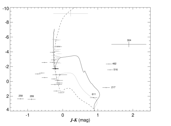
5 Multiplicity
We can use the total number of probable physical companions (column 3 of Table 5) to determine the multiplicity properites of our sample of 74 massive stars in Cyg OB2. There are 26 single (), 27 binary (), 12 triple (), and 9 higher multiplicity systems (). Note that we have essentially double counted the numbers in two cases where companions occur in two adjacent and overlapping fields, MT 213 + MT 217 (Schulte 4A,B) and MT 462 + MT 465 (Schulte 8A,B). The target with the largest number of companions (4) is MT 421 (Schulte 50) that resides at the center of a tentatively identified star cluster (Bica et al., 2003), so it it possible that some of the companions that met the criterion are cluster members that are not directly orbiting the central star.
The total multiplicity fraction (number of targets with any companion divided by the number of targets) and companion frequency (total number of companions divided by the number of targets) are summarized in Table 6 with uncertainties estimated as described by Aldoretta et al. (2015). The columns list the sample, a reference code, the number of primary targets , the range in physical separation of the detected companions given as the logarithm (base 10) of separation in Astronomical Units , the maximum magnitude difference of companions (max), , and . The top section of Table 6 lists our results and those of prior studies for companions that are angularly resolved. The lower section gives similar statistics by including closer systems discovered as spectroscopic binaries and/or eclipsing and ellipsoidal binaries (SB/E) in order to estimate the multiplicity properties over the full range of separation. The combined resolved and SB/E companion numbers are listed in column 6 of Table 5, and the resulting statistics are shown in the first row of the lower section of Table 6. The multiplicity fraction increases from to 0.65 by adding the known closely separated binaries, and likewise the companion frequency increases from to 1.11 with inclusion of the close systems. There are 29 known spectroscopic systems among our sample of stars (column 5 of Table 5), and resolved companions are more common in this subset ( and ) than among the full sample ( and ).
| Sample | Ref. aa 1. This paper and Caballero-Nieves et al. (2014); 2. Peter et al. (2012); 3. Gravity Collaboration et al. (2018); 4. Lafrenière et al. (2014); 5. Rizzuto et al. (2013); 6. Duchêne et al. (2001); 7. Aldoretta et al. (2015); 8. Sana et al. (2014); 9. Pomohaci et al. (2019); 10. This paper, Caballero-Nieves et al. (2014), and Kobulnicky et al. (2014). | (max) | ||||
|---|---|---|---|---|---|---|
| (AU) | (mag) | |||||
| Resolved Companions | ||||||
| Cyg OB2 | 1 | 74 | [2,4] | 9 | ||
| Cep OB2/3 | 2 | 148 | [2,3] | 7 | 0.25 | 0.27 |
| Orion Trapezium | 3 | 16 | [0,3] | 5 | 0.69 | 1.38 |
| Young Stars in Upper Sco | 4 | 91 | [1,3] | 10 | ||
| Sco OB2 B-type | 5 | 58 | [0,1] | 3 | 0.26 | 0.26 |
| NGC 6611 | 6 | 60 | [2,3] | 6 | ||
| Galactic OB in clusters/assoc. | 7 | 214 | [1,3] | 5 | ||
| Southern O-type | 8 | 96 | [0,4] | 8 | 1.5 | |
| Massive YSOs | 9 | 32 | [3,5] | 5 | ||
| Resolved + SB/E Companions | ||||||
| Cyg OB2 (all) | 10 | 74 | [,4] | 9 | ||
| Cyg OB2 () | 10 | 38 | [,4] | 9 | ||
| Cyg OB2 () | 10 | 27 | [,4] | 9 | ||
| Galactic OB in clusters/assoc. | 7 | 214 | [,4] | 5 | ||
| Southern O-type | 8 | 96 | [,4] | 8 | 2.1 | |
It is important to bear in mind that our reported statistics on angularly resolved binaries only include those companions above both the dotted (detection limited) and dashed lines (background limited) in Figure 1, so the and results in Table 6 should be regarded as lower limits because we miss systems outside of these limits. In particular, there is a systematic bias against detection of close and faint companions (Fig. 1). Consequently, it is very difficult to derive distributions of binary separation and mass ratio from our results. Furthermore, the magnitude-dependent characteristics of these limits may introduce some biases into our results, for example, with respect to stellar mass.
There is a well-known trend for the multiplicity fraction to increase with stellar mass (Duchêne & Kraus, 2013; Sana et al., 2014), and it is worthwhile examining whether or not this trend exists within our sample of Cyg OB2 stars. We divided the stars with mass estimates (column 8 of Table 5) into those below and above , and the statistics for these groups are given for the combined resolved plus SB/E companion numbers in rows 2 and 3 of the lower section of Table 6. We see that both and are larger in the higher mass group as expected for the trend of increasing multiplicity with stellar mass. We caution, however, that this mass dependence is partially due to selections effects. We show in Figure 1 the dividing lines for meeting the criterion for target stars with bright and faint magnitudes. These trends show that at larger separation the criterion will reject more and more brighter companions because of confusion with the background field. At the fainter apparent magnitude of the lower mass stars in our sample, the exclusion of candidate binaries becomes even more severe, so we expect that the multiplicity fraction will be lower for lower mass stars because of the greater difficulty in distinguishing their companions from the background stars. Consequently, the apparent increase in and with stellar mass in Table 6 is probably overestimated. Indeed, the statistics for the high mass group are probably more representative of the actual numbers, because the selection limits are more generous for the brighter, massive targets.
The upper part of Table 6 compares our multiplicity results with other earlier investigations from adaptive optics, Lucky Imaging, and interferometry. All these samples consist of massive or very young stars, similar to the composition of our Cyg OB2 sample. However, each of these surveys is sensitive to a particular range in angular separation and maximum magnitude contrast (columns 4 and 5, respectively, in Table 6), and in general those studies that cover a broader range in separation and magnitude difference yield higher multiplicity frequencies. Our results for and fall well within the range of these earlier studies, and higher values are only found from recent VLTI interferometric studies of the nearby Orion Trapezium (Gravity Collaboration et al., 2018) and southern O-type stars (Sana et al., 2014), and these studies span a relatively large range in separation and contrast sensitivity.
The lower part of Table 6 compares the statistics for the combined wide and close binary samples of Cyg OB2 with those from two all-sky surveys. Our results are broadly consistent with those from the HST/FGS survey of O-type stars by Aldoretta et al. (2015) for their subset of cluster and association members and with the VLTI/PIONIER and NACO/Sparse Aperture Masking survey of southern sky O-stars by Sana et al. (2014). In particular, if we adopt the results from the high mass group as the least affected by selection effects (see above), then our and results for Cyg OB2 appear to be consistent with these other surveys. Taken together, these studies imply that the massive stars in clusters and associations have a very large multiplicity frequency compared to lower mass stars (Duchêne & Kraus, 2013).
The high incidence of multiple systems among the more massive stars indicates that the angular momentum of the natal cloud is preferentially transformed into orbital motion (Larson, 2010). The processes involved in massive star formation are still the subject of active investigation (Rosen et al., 2020). The turbulent core model envisions the collapse of a virial natal cloud that creates widely spaced binaries accompanied by a small number of low mass stars formed by cloud fragmentation (Rosen et al., 2019). The stellar cores are surrounded by large disks, and disk fragmentation can lead to the formation of bound stellar companions (Kratter & Matzner, 2006). Subsequent disk accretion onto these companions can lead to the formation of close binaries (Lund & Bonnell, 2018; Tokovinin & Moe, 2020) that have much smaller separations than those investigated here. Alternatively, the competitive accretion model (Bonnell & Bate, 2006) suggests that massive stars form by accretion onto a cluster of low mass seeds in the dense, central regions of the natal cloud. These models tend to form star clusters where three-body encounters can create massive binaries over a wide range in separation (Wall et al., 2019). Both the turbulent core and competitive accretion models predict an increased binary fraction among more massive stars, but with somewhat different distributions in separation and mass ratio (Peter et al., 2012; Gravity Collaboration et al., 2018).
The subsequent dynamical interactions in small number clusters will generally lead to the formation a single, wide massive binary and the ejection of lower mass single stars (Griffiths et al., 2018). Wide binaries with separations of 100 to 10,000 AU are large enough for frequent gravitational encounters to occur in dense environments, and the large numbers of such wide binaries in Cyg OB2 indicates that they have survived potential disruptive encounters. Griffiths et al. (2018) argue that star formation in Cyg OB2 probably occurred in many well-separated locations in the natal cloud, so that close encounters with other cluster stars did relatively little damage to these wide binaries. This conclusion is bolstered by the fact that the binary frequency found in massive Young Stellar Objects (representing the frequency at birth) is similar to the present day binary frequency in Cyg OB2 (Table 6) even after several million years of dynamical evolution.
6 Conclusions
Our near-IR adaptive optics survey of the Cyg OB2 association has yielded astrometry and photometry for the fields surrounding 74 of its massive O- and B-type members. We find that of the sample of stars have a companion that is probably physically related. These companions have projected separations in the range from 100 to 19,000 AU, and the faintest companions detected are probably stars based upon their positions in the color - magnitude diagram. Many other closer companions must exist, and we included spectroscopic binary results from studies by Kobulnicky et al. (2014) that primarily sample systems with a semimajor axis range of 0.1 to 1 AU. The combined binary fraction is large even without accounting for systems in the relatively unexplored separation range of 1 to 100 AU. The derived multiplicity fraction is and the companion frequency is . We emphasize that these are lower limits to the actual fractions because our observations miss both very close and faint companions and because the fainter companions are indistinguishable from background stars. Nevertheless, our results are broadly consistent with earlier surveys of massive stars that include both spectroscopic (close) and resolved (wide) binaries. For example, the HST/FGS survey of O-type stars by Aldoretta et al. (2015) yielded and among cluster and association stars, and the VLTI/PIONIER and NACO/Sparse Aperture Masking survey of O-stars by Sana et al. (2014) led to and . This very high incidence of bound companions is consistent with the idea that massive star formation directs the angular momentum of the natal cloud into the creation of binary orbital motion.
The NIRI survey will help in the selection of targets for future adaptive optics and integral field unit spectroscopy observations to determine the physical properties of the companions. The close companion stars detected in the NIRI survey are especially interesting because their flux is blended into that of the main target for most ground-based observations that lack high angular resolution. Thus, the NIRI results can help correct the placement of these stars in the H-R diagram and can inform the interpretation of spectroscopy of hierarchical triples and other composite spectrum targets (see the case of MT 429; Kiminki et al. 2012). Finally, the closest resolved binaries hold the potential for orbital solutions and mass determination of the most massive stars. For example, S 5 = Cyg OB2 #5 is an hierachical system consisting of a central massive close binary, nearby tertiary, plus the two distant resolved companions (Rauw et al., 2019). The brightest and presumably most massive star in Cyg OB2 is MT 304 = Cyg OB2 #12, and both the close companion found by HST/FGS and the more distant companion found in the NIRI survey were detected in speckle observations by Maryeva et al. (2016), who claim that the close component has already displayed some orbital motion. The orbital period is probably yr, so continued high angular resolution observations hold the promise of weighing the most massive star in Cyg OB2 and one of the most massive stars in the Galaxy.
Appendix A NIRI/ALTAIR Astrometry Calibration
Each NIRI observation comes with World Coordinate System (WCS) information in the FITS header that is retained through the image reduction and coaddition process. These keywords list the pointing position and the right ascension and declination changes with pixel spacing along both axes. In principle, these can be used with the positions of stars in the merged image that were measured with SExtractor to derive the celestial coordinates . However, there are several complications that need to be considered. First, the pixel scale changed with the introduction of the field lens according to the Gemini Web site444http://www.gemini.edu/sciops/instruments/niri/imaging/pixel-scales-and-fov (see Table 7), but this change was neglected in the WCS header keywords. Second, there is an apparent barrel distortion in the NIRI camera images that causes stars at the periphery to appear closer to the center than they should based upon a strict linear plate scale (see notes at the Gemini Web site). Finally, it is important to make an independent check on the field rotation parameter in the FITS header.
We decided to verify the pixel scales and rotational zero point through a comparison of the relative positions with astrometry of the targets from the UK Infrared Telescope Infrared Deep Sky Survey (UKIDSS; Lawrence et al. 2007). The celestial coordinates in UKIDSS (J2000 equinox) are based upon stellar positions in the 2MASS survey (Skrutskie et al., 2006) and hence are indirectly related to the International Reference Coordinate System through the Tycho-2 system used by 2MASS (Lodieu et al., 2007).
Our goal was to obtain plate solutions for the field rotation and the - and -axis pixel scales from our positions and the corresponding UKIDSS coordinates for as many fields as possible. The first step was to remove the barrel distortion effects. We assumed that the main target occupied the axial central position, and that the radial distance of any other star from the image center equals the uncorrected linear distance from the main target. However, this is an approximation, because the dither pattern placed the target in the center in only one of the nine dither locations, and the star is displaced by 0 or pixels in and for the other dither placements. In fact, the distortion correction should actually be made before image coaddition to avoid variations in radial distance between the target and image center in the individual frames, but the dither offsets are small enough for our observations that the positional smearing that results from coaddition before barrel distortion correction only amounts to about one pixel at the edge of the FOV. The true radial distance corrected for barrel distortion is
where and is given in pixels (see Gemini Web site). Then the relative position from center may be transformed to a barrel distortion corrected position at
and
Next we obtained UKIDSS -band source data for the nominal position of the main target (from 2MASS) using a 15 arcsec search radius555http://surveys.roe.ac.uk:8080/wsa/region_form.jsp. The stellar positions were extracted from the UKIDSSDR7PLUS data release of the UKIDSS Galactic Plane Survey. We used the preliminary WCS header data to transform to to then match our targets with the sources in UKIDSS (where possible) based upon similar coordinates and magnitudes. Finally, we used the positional and coordinate data to obtain a plate solution using the IDL procedure astromit.pro (written by R. Cornett and W. Landsman666http://www.astro.washington.edu/docs/idl/idllib/obsolete/sunuit/lib/old/astromit.pro). The results for each field were collected in a file that listed the rotation angle and pixel scale in and for both the preliminary WCS data and the fit of the UKIDSS coordinates, plus the number of stars used in the fit.
We found that there were 49 fields where four or more stars were matched by sources in UKIDSS, and we used these to determine mean values of the pixel scales and rotational offsets that are summarized in Table 7 according to the field lens position (out for the 2005 observations and in for those from 2008). The first two rows give the expected pixel scales from the Gemini Web site and the work of Stoesz (2006), and the next two rows show the average of the and pixel scales according to the preliminary WCS keywords and the fit of the UKIDSS astrometry, respectively. The uncertainties quoted are the standard deviations of the mean in each case. We see that the pixel scales are close to the expected values, and the ratio of the fitted to WCS pixel scales (given in the fifth row as the WCS scale factor) is slightly less than one. Finally, there is a small but non-zero offset between the field rotational angle from the preliminary WCS keyword and the fits of the UKIDSS astrometry, .
| Parameter | Field lens out | Field lens in |
|---|---|---|
| Pixel scale [Gemini WWW] (mas pix-1) | 21.9 | 21.4 |
| Pixel scale [Stoesz 2006] (mas pix-1) | ||
| Pixel scale [WCS] (mas pix-1) | ||
| Pixel scale [fit] (mas pix-1) | ||
| WCS scale factor from fit | ||
| (deg) | ||
| Number of fields | 6 | 43 |
We used these calibration results to determine the to transformation using the IDL procedure xyad.pro777http://idlastro.gsfc.nasa.gov/ftp/pro/astrom/xyad.pro (written by W. Landsman) that we modified by performing the barrel distortion correction (see above), making a small rotation of the positions using for the lens in/out solutions in Table 7, and then rescaling the WCS pixel scales using the WCS scale factors for the lens in/out solutions in Table 7. The relative coordinates were then transformed to absolute using the 2MASS coordinates for the main target (J2000 equinox and ignoring the effects of proper motion between the times of the 2MASS survey and our observations). We caution that in some cases the 2MASS coordinates may actually represent the center of light position between the main target and a close companion, so that in such cases all the estimates may have systematic offsets. The relative positions should be regarded as our fundamental astrometric measurements. The target MT421 (Cyg OB2-22) was also observed by Maíz Apellániz (2010) using the Advanced Camera for Surveys (ACS) High Resolution Camera (HRC) on Hubble Space Telescope (red F850LP filter), and we compared the separations and position angles of the companions observed with HST and our calibrated astrometry to verify our calibration process. We found that the mean difference in fractional separation for five companions was and the mean difference in position angle was deg. Thus, our calibration of the astrometry leads to pixel scales that agree at the level and to systematic rotational differences at the deg level. The standard deviation between the rectilinear positions from the HST and NIRI astrometry is about 0.008 arcsec for these five companion stars, and this may represent the magnitude of any high-order geometric distortions that may exist in the NIRI ALTAIR astrometry system.
Appendix B NIRI/ALTAIR Photometry Calibration
The NIRI/ALTAIR images suffer from angular anisoplanatism that causes the point-spread function (PSF) to change from the center to the edge of the image. Stellar images near the periphery have relatively more flux in the halo surrounding the core than does a star image at the center. We measured stellar fluxes using aperture photometry with SExtractor for a series of apertures with diameters ranging from 5 to 80 pixels, and these represent a radial integration of the stellar PSF. Figure 4 shows an encircled energy (EE) plot of total flux measured versus aperture diameter for the case of a 2005 -band observation of MT 465. The solid line represents the EE curve for the target at the center of image and the dotted line shows the EE curve for another star offset by 431 pixels from the main target. We see that the PSF degradation of the offset star image results in a relative reduction in measured flux that is larger at smaller aperture size. Consequently, if we adopted a fixed aperture diameter of say 10 pixels for all our measurements, then we would systematically underestimate the flux of stars towards the edge of the field. On the other hand, if we used a larger diameter aperture (60 pixels or larger), then the differences in the EE flux with position would be insignificant. Unfortunately, the large aperture option is only practical with the brightest and isolated stars because the stellar signal becomes overwhelmed by background noise for faint stars measured with large apertures (often causing the EE curve to decline with increasing aperture; Howell 1989). Hence, we must apply an aperture correction scheme that accounts for the PSF degradation of our measurements.

The amount of PSF degradation depends on the radial position of the star, the jitter introduced by the coaddition of the individual frames, whether or not the NIRI field lens was used, and the air mass and seeing conditions at the time of the observation. Cresci et al. (2005) argue that a first order correction can be made for PSF degradation by considering a family of PSFs characterized by the ratio of the offset angle to the isoplanatic angle (dependent on air mass and seeing). Because the isoplanatic angle is inversely proportional to the astronomical seeing, this suggests that we may parameterize the changes in the EE curves using a parameter , where is the offset position from the target at the center of the image (measured in pixels) and is the FWHM of the astronomical seeing (recorded in the NIRI/ALTAIR header files as keyword AOSEEING). We first tested this idea by calculating EE curves for synthetic PSFs for NIRI/ALTAIR created with the PAOLA software package (Jolissaint, 2010), and we found that the ratio (where is the normalized enclosed energy for aperture and is the same for the main target at center) did indeed decline in an approximately linear fashion with both increases in radial offset and seeing. However, the observed PSFs have sufficiently different core structure from the model PSFs (presumably due to jitter that is not included in the models) that we decided to calibrate the change in the EE curves directly from our observations.
We implemented the aperture correction using the differential magnitude approach outlined by Stetson (1990) in which the instrumental magnitude difference between two apertures is
where is the flux estimated by SExtractor for an aperture of diameter . Uncertainties in were set by the flux uncertainties according to the from equation (1) of Howell (1989). This differential version of the EE curve is shown in the lower part of Figure 4. The advantange of using the differential form is that this magnitude difference may be estimated for the smaller apertures even for those faint stars where the EE curve is unreliable at larger apertures because of background noise (Stetson, 1990).
We then gathered measurements for all the aperture pairs for image samples selected by date (to account for the use or not of the field lens) and by filter band. In each case we formed the difference between for a given star and that for the central reference target, and we collected the offset parameter . The uncertainties in are estimated as , which reflects the typical scatter in seeing estimates among the subexposures. An uncertainty weighted fit was made of the function
for the first-order model of PSF degradation with parameter . The derived constants and their uncertainties are collected in Table 8 for each year and filter sample. The second row in the header indicates the associated aperture pair (by diameter in pixels) for each column. The PSF degradation trends are largest in the smaller aperture pairs, shorter wavelength filters, and data from 2005 when the AO field lens was not used. We also list in Table 8 similar coefficients for the PSF degradation observed in the PHARO images (made in 2009), but these should not be directly compared with the NIRI/ALTAIR results because the pixel scale is different and no seeing estimate was reported at the time, but based on AO performance, we estimate the data were taken in approximately seeing (Dekany et al., 2007).
| Image | ||||||||
|---|---|---|---|---|---|---|---|---|
| Set | (5–10) | (10–20) | (20–30) | (30–40) | (40–50) | (50–60) | (60–70) | (70–80) |
| 2005 | ||||||||
| 2005 | ||||||||
| 2005 | ||||||||
| 2008 | ||||||||
| 2008 | ||||||||
| 2009 | ||||||||
| 2009 | ||||||||
| 2009 | ||||||||
| (mag) | 0.162 | 0.049 | 0.022 | 0.010 | 0.009 | 0.010 | 0.014 | 0.017 |
Note. — Any negative values are assigned zero in practice.
We used the observed PSF degradation trends to estimate a model differential magnitude curve for each target’s position according to
where is the magnitude difference between apertures and for the central reference star, is the coefficient for a given date and filter (given in Table 8), and is the radial distance – seeing product. It is important to check how well this approximate treatment works in practice, so we compared the predicted curve with those observed for a subsample of 16 very bright and radially offset stars where the uncertainties due to photon and background noise are insignificant. The standard deviations of the observed minus model curves, , are given with each entry in Table 8, and these represent how well we might expect the model to perform in our application. In general these standard deviations are small but they are worse for the smallest aperture pairs where structure variations in the PSF are most pronounced. The full uncertainty in our estimate is given by
where the final term accounting for the off-axis correction is
The approximation used in the last step assumes that all the uncertainty in the product stems from the seeing uncertainty . The uncertainties in the coefficients are given with each entry of Table 8, and we adopt .
Now with the off-axis aperture curves in hand, we may estimate the magnitude difference between target and central reference star using an aperture correction as given by
where we refer all the fluxes to that in the largest, 80 pixel diameter aperture of the reference star. The uncertainty associated with this magnitude difference is
where is the uncertainty in the flux measurement expressed as a magnitude and are the uncertainties in the adopted curve as given above. Thus, we arrive at nine estimates of the magnitude difference and associated uncertainty from the measurements made in nine apertures. We select the estimate with the smallest uncertainty for our purposes in this paper, so that we can adopt the best compromise between large apertures for the bright stars (where the flux uncertainties are small compared to the aperture correction uncertainties) and smaller apertures for the fainter stars (where the flux uncertainties become huge in the large apertures). Note that stars at the periphery of the fields (i.e. stars that were not in all frames due to dithering) will have larger uncertainties than reported in Table 4.
We checked our scheme by comparing our derived differential -band magnitudes with those from the UKIDSS catalog for the populous field surrounding star MT 421. The individual stars were matched between the NIRI and UKIDSS sources according to our astrometry solution. Unfortunately, MT 421 itself is saturated in the UKIDSS data, so it is not possible to form magnitude differences from the UKIDSS data alone. Instead, we found the best fit magnitude offset needed to match the NIRI magnitude differences, and the implied magnitude of MT 421 is which is similar to the estimate from 2MASS, . We find that our corrected magnitudes and those from UKIDSS are in satisfying agreement with no evidence of systematic differences with magnitude. Furthermore, the scatter about the expected one-to-one relation is comparable to our uncertainty estimates, which suggests that our analytical representation of the uncertainties is reliable.
References
- Albacete Colombo et al. (2007) Albacete Colombo, J. F., Caramazza, M., Flaccomio, E., Micela, G., & Sciortino, S. 2007, A&A, 474, 495
- Aldoretta et al. (2015) Aldoretta, E. J., Caballero-Nieves, S. M., Gies, D. R., et al. 2015, AJ, 149, 26
- Bertin & Arnouts (1996) Bertin, E., & Arnouts, S. 1996, A&AS, 117, 393
- Bica et al. (2003) Bica, E., Bonatto, C., & Dutra, C. M. 2003, A&A, 405, 991
- Bonnell & Bate (2006) Bonnell, I. A., & Bate, M. R. 2006, MNRAS, 370, 488
- Bressan et al. (2012) Bressan, A., Marigo, P., Girardi, L., et al. 2012, MNRAS, 427, 127
- Caballero-Nieves et al. (2014) Caballero-Nieves, S. M., Nelan, E. P., Gies, D. R., et al. 2014, AJ, 147, 40
- Comerón et al. (2008) Comerón, F., Pasquali, A., Figueras, F., & Torra, J. 2008, A&A, 486, 453
- Comerón et al. (2002) Comerón, F., Pasquali, A., Rodighiero, G., et al. 2002, A&A, 389, 874
- Correia et al. (2006) Correia, S., Zinnecker, H., Ratzka, T., & Sterzik, M. F. 2006, A&A, 459, 909
- Cresci et al. (2005) Cresci, G., Davies, R. I., Baker, A. J., & Lehnert, M. D. 2005, A&A, 438, 757
- Czekaj et al. (2014) Czekaj, M. A., Robin, A. C., Figueras, F., Luri, X., & Haywood, M. 2014, A&A, 564, A102
- Dekany et al. (2007) Dekany, R., Bouchez, A., Roberts, J., et al. 2007, in Advanced Maui Optical and Space Surveillance Technologies Conference, E64
- Dekany et al. (2013) Dekany, R., Roberts, J., Burruss, R., et al. 2013, ApJ, 776, 130
- Duchêne & Kraus (2013) Duchêne, G., & Kraus, A. 2013, ARA&A, 51, 269
- Duchêne et al. (2001) Duchêne, G., Simon, T., Eislöffel, J., & Bouvier, J. 2001, A&A, 379, 147
- Fitzpatrick (1999) Fitzpatrick, E. L. 1999, PASP, 111, 63
- Gravity Collaboration et al. (2018) Gravity Collaboration, Karl, M., Pfuhl, O., et al. 2018, A&A, 620, A116
- Griffiths et al. (2018) Griffiths, D. W., Goodwin, S. P., & Caballero-Nieves, S. M. 2018, MNRAS, 476, 2493
- Hanson (2003) Hanson, M. M. 2003, ApJ, 597, 957
- Hayward et al. (2001) Hayward, T. L., Brandl, B., Pirger, B., et al. 2001, PASP, 113, 105
- Hodapp et al. (2003) Hodapp, K. W., Jensen, J. B., Irwin, E. M., et al. 2003, PASP, 115, 1388
- Howell (1989) Howell, S. B. 1989, PASP, 101, 616
- Jolissaint (2010) Jolissaint, L. 2010, Journal of the European Optical Society, 5
- Kiminki et al. (2015) Kiminki, D. C., Kobulnicky, H. A., Vargas Álvarez, C. A., Alexander, M. J., & Lundquist, M. J. 2015, ApJ, 811, 85
- Kiminki et al. (2007) Kiminki, D. C., Kobulnicky, H. A., Kinemuchi, K., et al. 2007, ApJ, 664, 1102
- Kiminki et al. (2012) Kiminki, D. C., Kobulnicky, H. A., Ewing, I., et al. 2012, ApJ, 747, 41
- Kobulnicky et al. (2012) Kobulnicky, H. A., Smullen, R. A., Kiminki, D. C., et al. 2012, ArXiv e-prints
- Kobulnicky et al. (2014) Kobulnicky, H. A., Kiminki, D. C., Lundquist, M. J., et al. 2014, ApJS, 213, 34
- Kratter & Matzner (2006) Kratter, K. M., & Matzner, C. D. 2006, MNRAS, 373, 1563
- Lafrenière et al. (2014) Lafrenière, D., Jayawardhana, R., van Kerkwijk, M. H., Brandeker, A., & Janson, M. 2014, ApJ, 785, 47
- Larson (2010) Larson, R. B. 2010, Reports on Progress in Physics, 73, 014901
- Lawrence et al. (2007) Lawrence, A., Warren, S. J., Almaini, O., et al. 2007, MNRAS, 379, 1599
- Le Bouquin et al. (2017) Le Bouquin, J. B., Sana, H., Gosset, E., et al. 2017, A&A, 601, A34
- Lodieu et al. (2007) Lodieu, N., Hambly, N. C., Jameson, R. F., et al. 2007, MNRAS, 374, 372
- Lund & Bonnell (2018) Lund, K., & Bonnell, I. A. 2018, MNRAS, 479, 2235
- Maíz Apellániz (2010) Maíz Apellániz, J. 2010, A&A, 518, A1
- Maíz Apellániz et al. (2016) Maíz Apellániz, J., Sota, A., Arias, J. I., et al. 2016, ApJS, 224, 4
- Maíz Apellániz et al. (2019) Maíz Apellániz, J., Trigueros Páez, E., Negueruela, I., et al. 2019, A&A, 626, A20
- Maryeva et al. (2016) Maryeva, O. V., Chentsov, E. L., Goranskij, V. P., et al. 2016, MNRAS, 458, 491
- Mason et al. (2009) Mason, B. D., Hartkopf, W. I., Gies, D. R., Henry, T. J., & Helsel, J. W. 2009, AJ, 137, 3358
- Mason et al. (2001) Mason, B. D., Wycoff, G. L., Hartkopf, W. I., Douglass, G. G., & Worley, C. E. 2001, AJ, 122, 3466
- Massey & Thompson (1991) Massey, P., & Thompson, A. B. 1991, AJ, 101, 1408
- Muntean et al. (2009) Muntean, V., Moffat, A. F. J., Chené, A. N., & de La Chevrotière, A. 2009, MNRAS, 399, 1977
- Negueruela et al. (2008) Negueruela, I., Marco, A., Herrero, A., & Clark, J. S. 2008, A&A, 487, 575
- Peter et al. (2012) Peter, D., Feldt, M., Henning, T., & Hormuth, F. 2012, A&A, 538, A74
- Pomohaci et al. (2019) Pomohaci, R., Oudmaijer, R. D., & Goodwin, S. P. 2019, MNRAS, 484, 226
- Raghavan et al. (2010) Raghavan, D., McAlister, H. A., Henry, T. J., et al. 2010, ApJS, 190, 1
- Rauw et al. (2019) Rauw, G., Nazé, Y., & Campos, F. 2019, A&A, 627, A2
- Richardson et al. (1998) Richardson, E. H., Fletcher, J. M., Morbey, C. L., Oschmann, J. M., & Pazder, J. S. 1998, in Proc. SPIE, Vol. 3353, Adaptive Optical System Technologies, ed. D. Bonaccini & R. K. Tyson, 600–610
- Rizzuto et al. (2013) Rizzuto, A. C., Ireland, M. J., Robertson, J. G., et al. 2013, MNRAS, 436, 1694
- Roberts & Singh (1998a) Roberts, S., & Singh, G. 1998a, in Adaptive Optical System Technologies, Vol. 3353, 611–620
- Roberts & Singh (1998b) Roberts, S., & Singh, G. 1998b, in Society of Photo-Optical Instrumentation Engineers (SPIE) Conference Series, Vol. 3353, Proc. SPIE, ed. D. Bonaccini & R. K. Tyson, 611–620
- Rosen et al. (2019) Rosen, A. L., Li, P. S., Zhang, Q., & Burkhart, B. 2019, ApJ, 887, 108
- Rosen et al. (2020) Rosen, A. L., Offner, S. S. R., Sadavoy, S. I., et al. 2020, Space Sci. Rev., 216, 62
- Rygl et al. (2012) Rygl, K. L. J., Brunthaler, A., Sanna, A., et al. 2012, A&A, 539, A79
- Sana et al. (2012) Sana, H., de Mink, S. E., de Koter, A., et al. 2012, Science, 337, 444
- Sana et al. (2013) Sana, H., de Koter, A., de Mink, S. E., et al. 2013, A&A, 550, A107
- Sana et al. (2014) Sana, H., Le Bouquin, J.-B., Lacour, S., et al. 2014, ApJS, 215, 15
- Schulte (1958) Schulte, D. H. 1958, ApJ, 128, 41
- Skrutskie et al. (2006) Skrutskie, M. F., Cutri, R. M., Stiening, R., et al. 2006, AJ, 131, 1163
- Stetson (1990) Stetson, P. B. 1990, PASP, 102, 932
- Stoesz (2006) Stoesz, J. A. 2006, PhD thesis, University of Victoria, Canada
- Straižys & Laugalys (2008) Straižys, V., & Laugalys, V. 2008, Baltic Astronomy, 17, 143
- ten Brummelaar et al. (2000) ten Brummelaar, T., Mason, B. D., McAlister, H. A., et al. 2000, AJ, 119, 2403
- ten Brummelaar et al. (1996) ten Brummelaar, T. A., Mason, B. D., Bagnuolo, Jr., W. G., et al. 1996, AJ, 112, 1180
- Tokovinin & Moe (2020) Tokovinin, A., & Moe, M. 2020, MNRAS, 491, 5158
- Torres-Dodgen et al. (1991) Torres-Dodgen, A. V., Carroll, M., & Tapia, M. 1991, MNRAS, 249, 1
- van der Hucht (2001) van der Hucht, K. A. 2001, New A Rev., 45, 135
- Wall et al. (2019) Wall, J. E., McMillan, S. L. W., Mac Low, M.-M., Klessen, R. S., & Portegies Zwart, S. 2019, ApJ, 887, 62
- Wright & Drake (2009) Wright, N. J., & Drake, J. J. 2009, ApJS, 184, 84
- Wright et al. (2012) Wright, N. J., Drake, J. J., Drew, J. E., et al. 2012, ApJ, 746, L21
- Wright et al. (2015) Wright, N. J., Drew, J. E., & Mohr-Smith, M. 2015, MNRAS, 449, 741
- Zinnecker & Yorke (2007) Zinnecker, H., & Yorke, H. W. 2007, ARA&A, 45, 481