A heavy molecular weight atmosphere for the super-Earth Men c
Abstract
Strongly irradiated exoplanets develop extended atmospheres that can be utilized to probe the deeper planet layers. This connection is particularly useful in the study of small exoplanets, whose bulk atmospheres are challenging to characterize directly. Here we report the 3.4-sigma detection of C ii ions during a single transit of the super-Earth Men c in front of its Sun-like host star. The transit depth and Doppler velocities are consistent with the ions filling the planet’s Roche lobe and moving preferentially away from the star, an indication that they are escaping the planet. We argue that Men c possesses a thick atmosphere with abundant heavy volatiles (50% by mass of atmosphere) but that needs not be carbon rich. Our reasoning relies upon cumulative evidence from the reported C ii detection, the non-detection of H i atoms in a past transit, modeling of the planet’s interior and the assumption that the atmosphere, having survived the most active phases of its Sun-like host star, will survive another 0.2–2 Gyr. Depending on the current mass of atmosphere, Men c may still transition into a bare rocky core. Our findings confirm the hypothesized compositional diversity of small exoplanets, and represent a milestone towards understanding the planets’ formation and evolution paths through the investigation of their extended atmospheres.
1 Introduction
Small exoplanets of sizes between Earth and Neptune are ubiquitous in the galaxy (Batalha, 2014),
yet intriguingly absent in our Solar System.
Even when their masses and radii are accurately known
(Fulton et al., 2017),
little can be confidently stated about their bulk compositions
(Seager et al., 2007; Valencia et al., 2010, 2013; Rogers & Seager, 2010; Nettelmann et al., 2011)
or the processes through which they form and evolve.
Men c is a close-in transiting super-Earth (Gandolfi et al., 2018; Huang et al., 2018)
(mass /=4.520.81; radius /=2.060.03;
orbital distance 0.067020.00109 AU)
expected to develop an extended atmosphere under the
significant XUV (=X-ray + Extreme Ultraviolet) stellar radiation that it receives (King et al., 2019; García Muñoz et al., 2020),
and is thus an ideal target to investigate the composition of small exoplanets.
Orbiting a Sun-like star, its study also potentially conveys insight into
our own Solar System.
Whereas planets with
radii 1.6 are likely rocky (composed of iron and silicates)
and those with 3 are expected to have a non-negligible amount of
light volatiles (H2/He) (Otegi et al., 2020),
Men c’s bulk density is consistent with an atmosphere that contains an admixture of light and
heavy (e.g. H2O, CO2, CH4, NH3) volatiles
(Rogers, 2015; Otegi et al., 2020),
which raises the interesting possibility that it may not be H2/He-dominated.
Compositional diversity is indeed predicted by theory (Fortney et al., 2013; Mordasini et al., 2015), and supported by the scatter in the
– statistics of known exoplanets (Hatzes & Rauer, 2015; Otegi et al., 2020).
Disentangling the composition of selected small exoplanets
is the key next step, and calls for a multiple line of evidence
approach that goes beyond and measurements.
Transmission spectroscopy at visible-infrared wavelengths provides
additional insight when gas absorption bands are revealed (Benneke & Seager, 2012).
However, when the measured spectrum is featureless (Guo et al., 2020),
it is difficult to discriminate between
atmospheres enshrouded by high-altitude clouds and atmospheres with abundant heavy volatiles.
Furthermore, the precision required for visible-infrared spectroscopy approaches the limit of
current and upcoming telescopes when
the band-to-continuum contrast drops below 20 parts per million (as for Men c).
Here, we alternatively constrain Men c’s bulk composition with
far-ultraviolet (FUV) transmission spectroscopy of selected atoms in its extended atmosphere
complemented with modeling of its interior structure and atmospheric mass loss.
The manuscript is structured as follows. In Section 2, we present new FUV transmission spectroscopy measurements of Men c and argue that the reported dimming originates in the planet’s atmosphere. In Section 3, we describe our upper atmosphere modeling, with emphasis on the net mass loss rate, the neutral/ionized state of the escaping hydrogen atoms, and their impact on atmospheric stability and detectability of hydrogen atoms. In Section 4, we describe our planetary interior modeling, which we use to estimate the atmospheric mass for different bulk compositions. Lastly, we invoke in Section 5 an argument of stability that connects the atmospheric mass with a time scale for the planet to lose it to escape. By requiring that this time scale is not much smaller than the system’s age, which would suggest fine-tuning in the evolution/current state of the planet, we are able to constrain Men c’s present-day atmospheric composition. Appendices A–D provide additional technical details.
2 HST/COS observations
We observed one FUV transit of Men c
with the Cosmic Origins Spectrograph (COS) aboard the Hubble Space Telescope (HST)
over five consecutive orbits (Program: GO-15699).
The first two orbits occurred before transit, the third orbit covered the ingress,
and the last two orbits occurred in transit with respect to the updated ephemeris.
For unknown reasons, the third observation returned no data.
The data were obtained in time-tag mode with the G130M grating centered at 1291 Å.
Each exposure lasted 3025 s, except the first one that was
2429 s because of target acquisition prior to the science observation.
Each spectrum covers the 1135–1429 Å range, with a gap between 1274 and 1291 Å.
For optimal stability during the observation,
we adopted one single instrumental Fixed Pattern position (FP-POS=3).
We downloaded the data from MAST, which were calibrated and extracted by calcos version 3.3.7111
https://www.stsci.edu/hst/instrumentation/cos/documentation/calcos-release-notes.
Each spectrum covers several stellar
lines of abundant elements (i.e., hydrogen, carbon, nitrogen, oxygen, silicon).
The lines of the O i 1302–1306 Å triplet, contaminated by geocoronal airglow,
were treated separately.
The H i Ly line was also severely affected by geocoronal airglow contamination
(HST/COS is particularly prone to this problem)
and gain sag and was not analyzed.
For each of the other spectral features,
we integrated the flux in wavelength to obtain a transit light curve for each line
and ion.
We either considered each line separately or added together the flux
from different lines of the same multiplet to increase the S/N
(i.e., for C iii, N v, C ii, and Si iv).
In this way, we constructed a transit light curve for each line and ion.
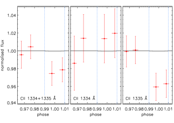
Among all light curves, we recorded a significant flux drop during transit only
for the triplet of C ii at 1334–1335 Å.
This feature is composed of a resonance line at 1334.532 Å and a doublet of components at
1335.663 and 1335.708 Å arising from an excited state (0.007863 eV).
This is why for nearby stars only the bluest line of the triplet is affected by ISM absorption
(furthermore in the nearby ISM, C ii is the dominant C ion (Frisch & Slavin, 2003)).
The C ii 1335-Å doublet is unresolved with COS and the line at 1335.663 Å is about
10 weaker than the line at 1335.708 Å, which is the strongest of the triplet.
The resonance line at 1334.532 Å is intrinsically about 1.8 times weaker than the
1335.708 Å line.
In our analysis we ignored the weakest component at
1335.663 Å. The light curves obtained from splitting the two main lines further
indicated that the absorption signal was induced by the C ii 1335 Å line
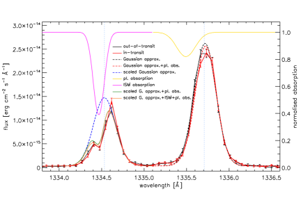
(Figure 1, top).
Considering only the C ii 1335 Å line, the transit depth integrated across the
whole line (i.e., 146 km/s from the line center) is 3.91.1%.
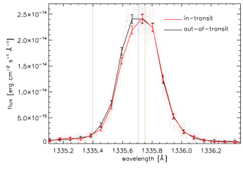
We averaged the in-transit and out-of-transit data separately to obtain one
master in-transit and one master out-of-transit spectrum and identify the velocities at
which the absorption in the C ii 1335 Å feature occurs.
Figure 1 (bottom) compares the in- and out-of-transit spectra.
The C ii 1335 Å feature shows in-transit dimming for velocities between 70 and 10 km/s.
The corresponding transit depth over this velocity range is 6.82.0% (3.4 sigma detection).
The corresponding flux drop at the 1334 Å line could not be detected because of interstellar medium absorption (ISM).
We also unsuccessfully looked for absorption in this same velocity range for all the other stellar features
(Table 1).
Appendix A provides further insight into the COS data analysis,
and discusses the masking of the C ii 1334 Å line by the ISM,
the unlikeliness that the reported in-transit dimming is caused by random fluctuations
in the stellar line shape and the search for in-transit dimming at the O i 1302–1306 Å triplet.
Our tests suggest that the stellar C ii line does not exhibit intrinsic temporal variations
and therefore that the C ii 1335 Å line dimming is caused by the planet transit.
Ideally, future HST/COS observations over one or more transits will confirm the above.
The confirmation is obviously important for Men c but also to set useful precedents
in the investigation of other small exoplanets with FUV transmission spectroscopy.
We attribute the dimming of the C ii 1335 Å line to absorption by
C ii ions escaping Men c along with other gases,
even though the signatures of the other gases are not directly seen in our data.
Our detection adds to a growing list of exoplanets with extended atmospheres
(Vidal-Madjar et al., 2003; Fossati et al., 2010; Ben-Jaffel & Ballester, 2013; Linsky et al., 2010; Ehrenreich et al., 2015; Bourrier et al., 2018b).
Unlike Men c, there is strong evidence that these other exoplanets’ atmospheres
are H2/He-dominated.
The transit depth and Doppler velocities reported here are consistent with the C ii ions being swept by
the stellar wind into a 15-wide
(about the extent of the Roche lobe in the substellar direction,
and closer to the planet than the interface between the planetary and stellar winds)
tail and accelerated to high velocities, a scenario suggested by
3D models of Men c and other exoplanets (Shaikhislamov et al., 2020a, b).
We found by means of a simplified phenomenological model of Men c’s tail (Appendix B) that the
C ii measurements can be explained if the planet loses carbon at a rate 108 g s-1,
requiring that the atmosphere contains this atom in at least solar abundance.
A tail-like configuration facilitates the detection, but
saturation of the absorption signal impedes setting tighter constraints
on the C ii abundance when it becomes supersolar. In summary,
we cannot yet conclude
whether carbon is a major or minor constituent of Men c’s atmosphere.
Future 3D modeling that incorporates all the relevant physics for the escaping
atmosphere (including the C ii ions) and its interaction with the star
may help discern amongst atmospheric compositions with various carbon abundances.
3 Extended atmosphere
A prior observation of Men c with the HST Space Telescope Imaging Spectrograph (STIS) revealed no evidence for in-transit absorption of the stellar Ly line (García Muñoz et al., 2020). When present, absorption in the Ly wings is primarily caused by energetic neutral atoms (ENAs) (Holmström et al., 2008; Tremblin & Chiang, 2013), which are fast neutral hydrogen atoms generated when the low-velocity neutral hydrogen escaping the planet and the high-velocity protons in the stellar wind exchange charge:
3D modeling shows that if Men c’s atmosphere is H2/He-dominated,
large amounts of ENAs are generated that produce measurable Ly transit depths
(Shaikhislamov et al., 2020b).
Conversely,
reduced ENA generation occurs if either the flux of stellar wind protons or the flux
of neutral hydrogen from the planet are weak. The arrangement of C ii ions
into a tail suggests that the stellar wind is not weak, and thus we disfavor the first
possibility.
A weak neutral hydrogen flux from the planet (the slow component of the above reaction)
suggests that hydrogen is not the major
atmospheric constituent or that it ionizes before interacting with
the stellar wind.
We investigated Men c’s extended atmosphere and mass loss with a photochemical-hydrodynamic model (García Muñoz et al., 2020).
The model takes as input the volume mixing ratio (vmr)
at the 1 bar pressure level for each species in the chemical network.
Photo-/thermochemical considerations (Moses et al., 2013; Hu & Seager, 2014) dictate the most
abundant molecules in the bulk atmosphere given the equilibrium temperature and the
fractions of hydrogen, helium, carbon and oxygen nuclei (, ,
, ;
defined as the number of nuclei (symbol ∗) of each element divided by the total number of nuclei).
For Men c’s 1150 K,
the bulk atmosphere composition is dominated by H2 provided that 1.
For lower values,
other molecules become abundant, such as H2O, CO, CO2 and O2 if
/1, or C2H2 and CO if /1.
To identify the dominant gases
in the bulk atmosphere for given sets of nuclei fractions and specify their
vmrs at the 1 bar pressure level,
we used a published study of super-Earths and
sub-Neptunes (Hu & Seager, 2014) (in particular their Figure 7).
We considered bulk compositions in which hydrogen nuclei dominate,
and compositions in which carbon and oxygen nuclei are also abundant and combine into
various molecules.
Table 2 of Appendix C summarizes
the implemented vmrs and other derived information
for the battery of 30 atmospheric runs (labelled as cases 01–30) that we performed.
Further details on our extended atmosphere modeling are provided in Appendix C.
For the conditions explored here,
the minimum and maximum loss rates are 1 and 3% /Gyr. The loss rates
depend weakly on composition even though the partitioning into different escaping nuclei can be very different.
Our models indicate that the neutral hydrogen flux (the slow component for ENA generation, see above)
at a reference location defined by the sonic point
is (Mach=1)5 g s-1
for H2/He-dominated atmospheres.
From published 3D models for H2/He-dominated atmospheres
incorporating ENAs (Shaikhislamov et al., 2020b; Holmström et al., 2008),
we estimate that a neutral hydrogen flux about 1/4 that value will bring the ENA generation
in line with the non-detection of Ly absorption.
Thus,
we set (Mach=1)1.25 g s-1 as the approximate
threshold for bulk compositions
consistent with insufficient ENA generation and therefore with the
non-detection of Ly absorption.
Refining this approximate threshold requires the 3D modeling of Men c’s atmosphere
for a diversity of bulk compositions, which should be the focus of future
investigations. Although welcome, such refinements will not modify the key
findings of this work.
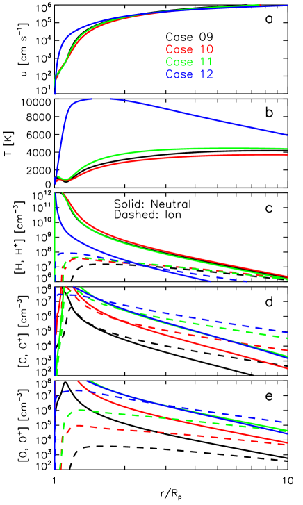
The flux (Mach=1) depends strongly on the
mass fraction of heavy volatiles in the atmosphere (=mass of heavy volatiles
relative to the mass of all volatiles), especially for 0.4 when hydrogen
becomes preferentially ionized due to high temperatures (Figure 2)
(see also Fig. 4 in García Muñoz et al., 2020).
Remarkably, (Mach=1) depends weakly on
the identity of the gases contributing to ,
and indeed the calculated fluxes are comparable for each subset of atmospheric runs with
different / ratios.
We exploit the model-predicted –(Mach=1) relation
(purple line in Fig. 3, right axis: top panel for cases 01-06;
bottom panel for cases 07-12)
to infer that Men c’s atmosphere has a high
(0.85 based on our approximate threshold for (Mach=1),
although the precise is subject to the prescribed threshold),
as otherwise the HST/STIS observation would have revealed Ly absorption.
The trend for –(Mach=1) in Fig. 3
reflects that the partitioning between neutral and ionized hydrogen varies by a larger factor
than the net mass loss rate (which varies by 3 for the explored ).
4 Bulk atmosphere
We built interior structure models of Men c that are consistent with its
, and using a tested methodology (Nettelmann et al., 2011; Poser et al., 2019).
The models are organized into a rocky core of iron and silicates in terrestrial proportions,
and an atmosphere on top containing H2/He plus a single heavy volatile
(CO2 or H2O, thus bracketing a broad range of molecular weights).
This core composition produces – curves for atmosphereless objects
consistent with the known exoplanets
that presumably lack a volatile envelope (Otegi et al., 2020).
When considering H2O as the dominant heavy volatile, it is assumed that
another carbon-bearing molecule present in trace amounts carries the carbon detected in
the HST/COS data. We assume that all gases remain well mixed,
which is justifiable for reasonable values of the eddy diffusion
coefficient in the atmosphere and the mass loss rates estimated here (García Muñoz et al., 2020).
The H2/He mass fraction is kept constant to the protosolar value,
but is varied to explore atmospheres with different abundances of heavy volatiles.
We can thus pair the interior structure models and the upper atmosphere
models on the basis of their corresponding and the dominating molecules (or more generally the
/ ratio in the upper atmosphere).
The models consider a present-day intrinsic temperature (, which specifies the heat flux from the
interior through Stefan-Boltzmann’s law ) and an extra opacity
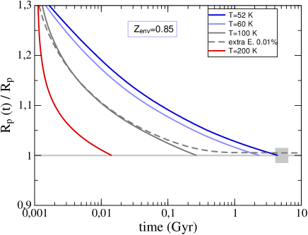
as adjustable parameters. We find that for 100 K all plausible atmospheres are relatively
light and would reach the current state within a time much shorter than the system’s age
(5.21.1 Gyr) and then would continue cooling and contracting
(Fig. 8, top left).
We consider this temperature to be a conservative upper bound.
Remarkably, for all other parameters being the same,
a higher translates into a less massive atmosphere that is easier to lose.
Indeed, increasing
causes larger scale heights and in turn larger atmospheric volumes for the same atmospheric mass.
The best match betwen evolution models that include stellar irradiation
as the sole external energy source and the measured after cooling for 3 Gyr
occurs for =44–52 K (Fig. 8, top left),
in which case the atmosphere has reached equilibrium with the incident irradiation.
In what follows, we focus on the range =44–100 K.
Key model outputs are the atmosphere and core masses
(+=) and the core radius ().
These quantities (, ) are determined with no prior assumption
on their values by iteratively solving
the interior structure equations so that upon convergence the model complies with the specified planet mass and radius
constraints.
For reference, the core size turns out to be always /1.6 for 1,
but can be 1.4 for (H2O)=0.9 and
1 for (CO2)=0.9.
Appendix D provides additional insight into the interior structure model.
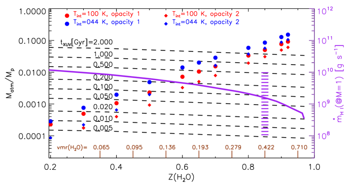
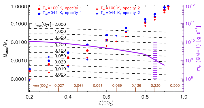
H2/He-dominated atmospheres (1) are more voluminous but overall contribute little mass (Figure 3, left). For example, /210-3 for (H2O) or (CO2)=0.3. In turn, an atmosphere with abundant heavy volatiles must be massive to compensate for its reduced scale height. Thus, /710-2 for (H2O)=0.8, and as high as 0.2 for (CO2)=0.8. However, not every atmospheric composition consistent with the interior models is stable over long timescales. We estimated the mass of atmosphere that is lost over a range of times as / (dashed lines, Figure 3), where is the loss rate predicted by our photochemical-hydrodynamic models and that varies as the stellar XUV luminosity and the planet orbital distance evolve. We incorporate these effects into , which must be viewed as an equivalent time based on the current stellar luminosity and orbit.
5 Atmospheric stability and composition
Using arguments of atmospheric stability to constrain Men c’s interior
requires an appropriate timescale over which the atmosphere will survive.
We first adopted a survival time of 2 Gyr, which is a moderate fraction of the
time left before the star exits the main sequence (5 Gyr) and assumes that
Men c is not near catastrophic mass loss.
This choice implicitly assumes that if the atmosphere survived the
100–1000 enhancement in XUV luminosity experienced in the early
life of its host star, then its end might not be imminent.
Under this hypothesis, we infer (Figure 3)
that (H2O)0.73 and (CO2)0.65.
These are conservative bounds based on the uppermost sets of
interior model curves for each heavy volatile, and correspond to volume mixing ratios vmr(H2O)0.26 (molecular weight
6.4 g mol-1) and vmr(CO2)0.09 (6 g mol-1).
A ten-fold shorter survival time results in
(H2O)0.50 (vmr(H2O)0.11; 4.1 g mol-1) and
(CO2)0.45 (vmr(CO2)0.04; 4 g mol-1).
The inferred heavy mass fractions are approximately consistent with the non-detection
of Ly absorption, which renders independent support to our findings. It ultimately confirms
that a thick atmosphere with more than half its mass in
heavy volatiles is a realistic scenario for Men c.
For comparison, maximum values of vmr(H2O)0.09–0.15 have been inferred
from infrared spectroscopy for the only other exoplanet with 3
at which H2O has been detected (Benneke et al., 2019; Tsiaras et al., 2019; Madhusudhan et al., 2020).
Thus, Men c becomes the exoplanet with the highest abundance of heavy volatiles known to
date, and its case suggests that even higher abundances might be expected
for other small exoplanets.
It is uncertain how the planet acquired such a heavy atmosphere, although high-
atmospheres are natural outcomes of formation models (Fortney et al., 2013).
Assuming that water is the dominant heavy volatile, it is plausible that Men c might have formed beyond the snow line
and reached its current orbit following high-eccentricity migration and tidal circularization.
The idea is supported by Men c being on a misaligned orbit with respect
to the stellar spin axis (Kunovac Hodžić et al., 2020)
and the fact that the system contains a far-out gas giant on an eccentric, inclined orbit
(Damasso et al., 2020; De Rosa et al., 2020; Xuan & Wyatt, 2020).
Men c lies near the so-called radius gap (Owen & Wu, 2013; Fulton et al., 2017)
that separates the population of planets
that presumably lost their volatiles through atmospheric escape
(peak at /1.5)
from those that were able to retain them (peak at /2.5).
The planet may still lose up to 10% of its mass
in the future 5 Gyr if it remains on its current (and stable) orbit (De Rosa et al., 2020; Xuan & Wyatt, 2020).
This is more than what the planetary interior models predict for /
for some plausible atmospheric configurations.
It is thus likely that we are witnessing Men c while crossing the radius gap.
Indeed, Figure 3 suggests that this will happen unless
the actual (H2O)0.85 or (CO2)0.80.
In that event, and because /1 for such unstable
configurations, the remnant core will collapse onto the empirical
– curve for atmosphereless objects.
| Ion | Wavelength | In-transit | Statistical |
| [Å] | absorption [] | significance | |
| C ii | 1335.7 | 6.762.00 | 3.39 |
| O i | 1302.168 | 3.6540.65 | 0.09 |
| O i | 1304.858 | 8.336.32 | 1.32 |
| O i | 1306.029 | 5.173.66 | 1.41 |
| Si iii | 1206.5 | 1.492.01 | 0.74 |
| N v | 1238.821 | 0.825.37 | 0.15 |
| N v | 1242.804 | 17.269.97 | 1.73 |
| Si ii | 1265.002 | 3.384.94 | 0.68 |
| Cl i | 1351.656 | 6.127.65 | 0.80 |
| O i | 1355.598 | 7.365.87 | 1.25 |
| Si iv | 1393.755 | 8.413.09 | 2.72 |
| Si iv | 1402.770 | 0.535.07 | 0.11 |
| All ions excluding | 2.671.27 | 2.10 | |
| C ii and O i triplet |
Appendix A Preparation of the observations and data analysis
We improved the published transit ephemeris (Gandolfi et al., 2018)
using TESS data from Sectors 1, 4, 8, 11–13 and the code pyaneti (Barragán et al., 2019),
which allows for parameter estimation from posterior distributions.
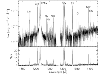
Figure 4 shows the spectrum obtained during the second HST observation (top),
marking the stellar features at which we looked for absorption in the 70 to 10 km/s velocity range,
and the resulting signal-to-noise ratio per spectral bin (middle).
The bottom panel compares the in- and out-of-transit spectra.
Having detected absorption of the C ii 1335 Å feature, we looked for a
similar signal at the C ii 1334 Å line, without success.
Next, we show that the absorption signal at 1334 Å is hidden by ISM contamination
(Figure 4, bottom), which affects the S/N.
We first fitted the C ii 1335 Å stellar feature using a Gaussian profile
and the out-of-transit spectrum (black dashed line) and then employed a further Gaussian profile to
fit the position and strength of the planetary
absorption on the in-transit spectrum (yellow solid line).
We obtained that the Gaussian profile simulating the planetary absorption lies at a velocity of
about 48.5 km/s with respect to the position of the main C ii 1335 Å feature,
has a normalized amplitude of 0.18, and a width of 0.11 Å.
These fits were performed considering the unbinned spectra.
We then derived the strength of the C ii 1334 Å line, prior to ISM absorption by
scaling the Gaussian fit to the C ii 1335 Å feature by the ratio of the oscillator
strength times the statistical weight of the two lines (about 1.8; blue dashed line).
We further simulated the C ii ISM absorption profile at the position of the C ii
1334 Å resonance line employing a Voigt profile (purple solid line),
in which we set the position of the line equal to that obtained
from the reconstruction of the stellar Ly line (García Muñoz et al., 2020)
and a C ii ISM column density equal to that of hydrogen
scaled to the expected ISM carbon-to-hydrogen abundance ratio and ISM C ionization fraction
(Frisch & Slavin, 2003) (green solid line).
Figure 4 (bottom) indicates that the simulated profile is a good
match to the out-of-transit spectrum, particularly accounting for the uncertainties
involved in inferring the C ii ISM column density. Finally, we added to this line the
planetary absorption obtained from fitting the C ii 1335 Å feature,
rescaled by 1.8 (orange solid line).
Lastly, Figure 4 (bottom) shows that the difference between the simulated
C ii 1334 Å line profiles before and after adding the planetary absorption is
significantly smaller than the observational uncertainties and hence undetectable in the data.
In summary, reduced S/N due to ISM contamination hides the planetary absorption signal at 1334 Å.
To estimate the likelihood that our C ii signal is due to intrinsic stellar
variability, we did a Monte Carlo simulation where we assumed the population of
intrinsic stellar variability between the mean in-transit and mean out-of-transit spectrum
is represented by the measured in-transit absorption from each line (Table 1).
We excluded from this representative population the C ii lines because of the putative
planetary absorption and the O i triplet because the noise properties and intrinsic
variability of these airglow-contaminated lines are different.
For the remaining eight emission lines, we calculate a weighted mean of
2.671.27% for the in-transit absorption. We made 106 realizations of nine emission
lines (the eight ’unaffected’ lines of the representative population plus C ii 1335.7 Å,
the line with the 3.4-sigma in-transit absorption) each with in-transit absorption
randomly drawn from a normal distribution with mean 2.67% and standard deviation 1.27%.
We find that the likelihood of 1 or more emission lines having an absorption 6.76%
due to intrinsic stellar variability as measured by our COS spectra is 2%.
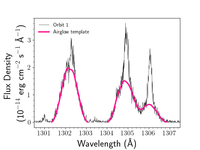
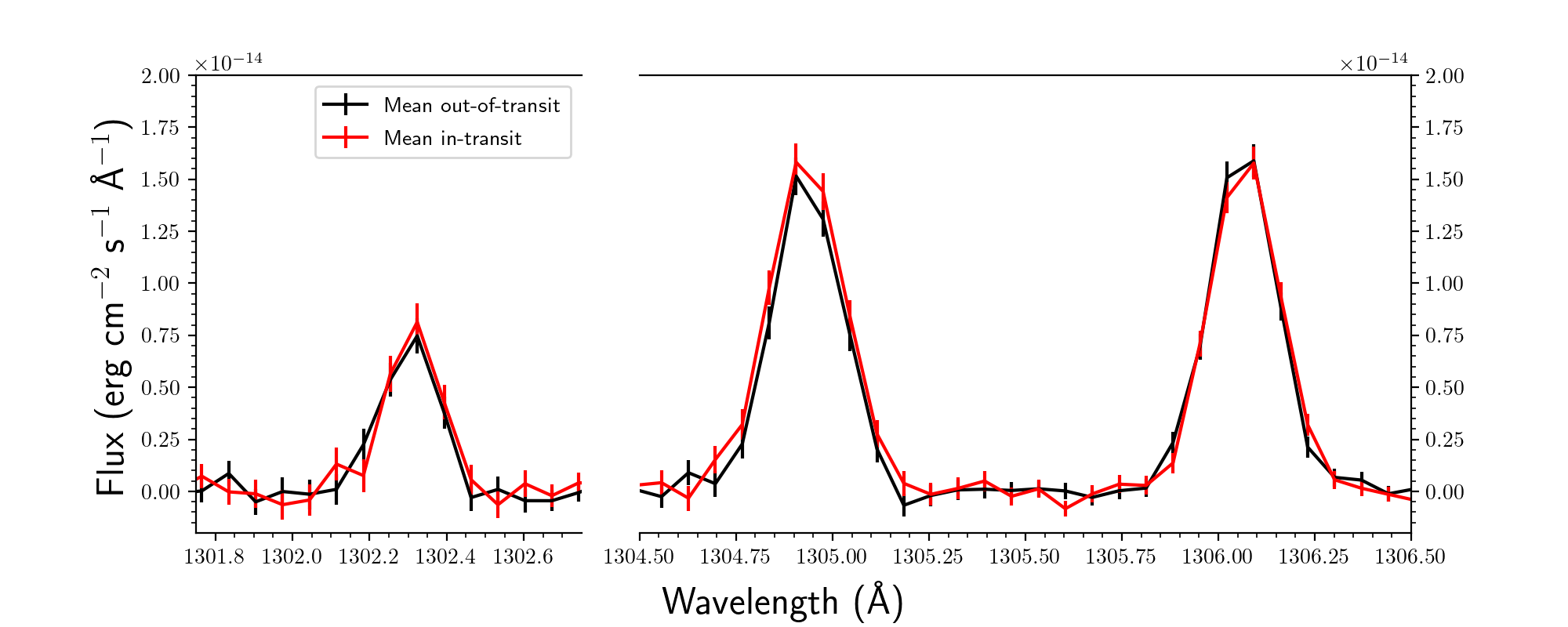
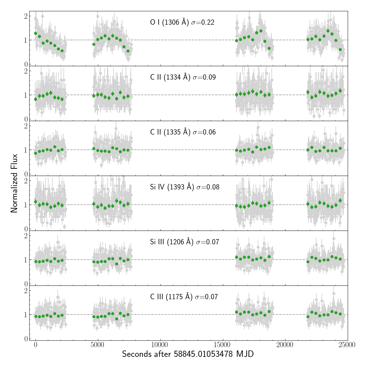
We inspected the O i lines for evidence of planetary absorption. The O i triplet at 1302–1306 Å is comprised of three emission lines that share an upper energy level. O i 1302.168 Å is the resonance line, and is significantly affected by ISM absorption. O i 1304.858 and 1306.029 Å each have similar oscillator strengths to the resonance line. COS’s wide aperture leads to significant contamination of each line of the O i triplet by geocoronal airglow. We corrected each orbit’s pipeline-reduced x1d spectrum’s O i emission lines for geocoronal airglow by performing a least-squares fit of the airglow templates downloaded from MAST (Bourrier et al., 2018a) to the spectrum (Figure 5, top). We created mean in-transit and out-of-transit spectra in the same way as the C ii lines, and measured absorptions in each of the three lines (shortest wavelength to longest wavelength) of 3.6540.65 %, 8.336.32%, and 5.173.66% over the same velocity range as C ii (Figure 5, bottom). No significant variation was observed in the O i triplet. The O i line at 1355 Å similarly does not show any significant variation between in-transit and out-of-transit. Lastly, we produced time series for the flux of some stellar lines (Figure 6). The series reveals no obvious variability that could cause a false transit detection.
Appendix B Phenomenological model of the ion tail
Our nominal transit depth for C ii of 6.8% translates into a
projected area equivalent to a
disk of radius /=15.1.
This is about the extent of Men c’s Roche lobe in the substellar direction
(/=13.3).
The spectroscopic velocity of 10 km/s for the C ii ions is consistent with our photochemical-hydrodynamic predictions,
and likely traces absorption in the vicinity of the planet’s dayside
as the gas accelerates toward the star.
Comparable velocities are predicted by 3D models on the
planet’s dayside (Shaikhislamov et al., 2020b)
before the escaping gas interacts with the impinging stellar wind.
Negative velocities of 70 km/s (and probably faster, as the stellar line becomes
weak and the S/N poor at the corresponding wavelengths)
suggest that the C ii ions are accelerated away from the star by other mechanisms such as
tidal forces and magnetohydrodynamic interactions with the stellar wind.
For reference,
the velocity of the solar wind at the distance of Men c is on the order of 250 km/s
(Shaikhislamov et al., 2020b).
There is observational evidence for HD 209458 b,
GJ 436 b and GJ 3470 b that their escaping atmospheres
also result in preferential blue absorption (particularly the latter two)
(Vidal-Madjar et al., 2003; Ehrenreich et al., 2015; Bourrier et al., 2018b).
Models considering the 3D geometry of the interacting stellar and planet winds
also favor blue absorption,
especially when the stellar wind is stronger (Shaikhislamov et al., 2020a, b) and arranges
the escaping atoms into a tail trailing the planet.
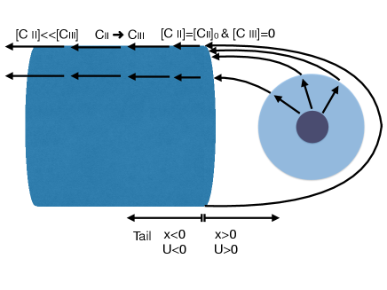
We consider a C ii tail to be realistic scenario for Men c.
To gain intuition, we have built the phenomenological model
of Men c’s tail sketched in Figure 7 (top).
The C ii ions are injected into a cylindrical tail of fixed radius 15
and are subject to a prescribed velocity =( /) km/s
that varies in the tail direction.
This geometry surely simplifies the true morphology of the escaping gas,
which is likely to resemble an opening cone tilted with respect to the star-planet line
(Shaikhislamov et al., 2020b). This crude description allows us at the very least to
obtain analytical expressions for some of the relevant diagnostics.
Here, =10 km/s (a typical value from the photochemical-hydrodynamic simulations;
Figure 2) and is an acceleration time scale.
(Note: 0 in the tail, and the ions are permanently accelerating.)
Related accelerations have been predicted by physically-motivated 3D
models (Ehrenreich et al., 2015; Shaikhislamov et al., 2020a, b), under
the combined effect of gravitational, inertial and radiative forces.
Magnetic interactions with the stellar wind might additionally affect ion acceleration.
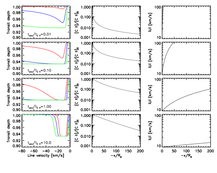
The C ii ions photoionize further into C iii with a time scale 20 hours (calculated for unattenuated radiation from Men at wavelengths shorter than the 508-Å threshold and the corresponding C ii cross section (Verner & Yakovlev, 1995)). The collision of stellar wind particles with the planetary C ii ions might ionize further the latter (ionization potential of 24 eV), especially at the mixing layer between the two flows (Tremblin & Chiang, 2013), but it remains unclear whether collisional ionization can compete on the full-tail scale with photoionization. This should be assessed in future work. The continuity equations that govern the model are:
As the flow accelerates through the tail, the total density decays and the C ii ions are converted into C iii. The solution for the C ii ion number density is:
This highly simplified exercise aims to estimate reasonable values
for the free parameters [C ii]0 and that reproduce
the transit depth and Doppler velocities from the COS data.
To produce the wavelength-dependent opacity,
we integrate [C ii]() along the line of sight keeping track of the Doppler shifts introduced
by the varying ().
We represent the C ii cross section at rest for the 1335.7 Å line by
a Voigt lineshape with thermal (=6000 K, a reference temperature in the tail;
our findings do not depend sensitively on this temperature,
as the absorption over a broad range of velocities is caused by the bulk velocity of the ions
rather than by their thermal broadening) and natural
(Einstein coefficient =2.88108 s-1) broadening components,
and a fractional population of the substate from which the line arises based on
statistical weights and equal to 2/3.
Figure 7 (bottom) shows how [C ii]0 and /
affect the absorption of the stellar line.
Absorptions consistent with the measurements are generally found for
[C ii]0104 cm-3 and /1, and
result in C ii tails longer than 50 and large amounts of C ii
moving at 70 km/s.
A key outcome of the model is that
for /1 the C ii ion photoionizes too quickly to
produce significant absorption at the faster velocities. This could in principle be
compensated with increasing amounts of C ii ions entering the tail, but the
photochemical-hydrodynamic model indicates that it is not possible to go
beyond [C ii]0106 cm-3 without obtaining unrealistically large
escape rates.
For [C ii]0104106 cm-3, the mass fluxes of carbon atoms through the
tail range from 108 to 1010 g s-1.
These mass fluxes are comparable to the loss rates of carbon nuclei predicted by our
photochemical-hydrodynamic model for atmospheres that
have carbon abundances larger than solar (Table 2).
This sets a weak constraint on the carbon abundance that
prevents us for the time being from
assessing whether carbon is a major constituent of Men c’s atmosphere.
This insight into Men c’s carbon abundance, even though of limited diagnostic value, is consistent with the interpretation of in-transit absorption by C ii at the hot Jupiter HD 209458 b (Vidal-Madjar et al., 2004; Ben-Jaffel & Sona Hosseini, 2010; Linsky et al., 2010). Both HD 209458 b and Men c transit Sun-like stars and exhibit similar transit depths. 3D models of HD 209458 b (Shaikhislamov et al., 2020a) show that its C ii absorption signal is explained by carbon in solar abundance. Because the predicted mass loss rate of HD 209458 b is an order of magnitude higher than for Men c (a result mainly from its lower density), a reasonable guess is that a 10 solar enrichment for Men c will result in comparable transit depths. Future 3D modeling of the interaction of the C ii ions with the stellar wind and the planet’s magnetic field lines should help refine these conclusions.
Appendix C Photochemical-hydrodynamic model
We investigated Men c’s extended atmosphere
with a 1D photochemical-hydrodynamic model that
solves the gas equations at pressures 1 bar (García Muñoz et al., 2020).
Heating occurs from absorption of stellar photons by the atmospheric neutrals.
Cooling is parameterized as described in our previous work, and
includes emission from H in the infrared,
Ly in the FUV, atomic oxygen at 63 and 147 m, and rotational cooling from
H2O, OH and CO also in the infrared.
We adopted a NLTE formulation of H cooling that
captures the departure of the ion’s population from equilibrium at low H2 densities.
We included a parameterization of CO2 cooling at 15 m (Gordiets et al., 1982).
The model considers 26 chemicals
(H2, H, He, CO2, CO, C, H2O, OH, O, O2,
H, H+, H, He+, HeH+, CO, CO+, C+, HCO, HCO+,
H2O+, H3O+, OH+, O+, O and electrons) that
participate in 154 chemical processes.
It does not include hydrocarbon chemistry,
although this omission is not important as hydrocarbons are
rapidly lost at low pressures in favor of other carbon-bearing species
(Moses et al., 2013).
To explore a broad range of compositions, we adopted nuclei fractions
and such that
+ goes from a few times 10-6 to 0.4,
and / ratios from 0.1 to 10.
We imposed =0.1.
By definition +++=1, and
thus the composition is specified by only two nuclei fractions.
With the above information, we estimated the corresponding vmrs from Figure 7 of Hu & Seager (2014)
and assigned them as boundary conditions of our extended atmosphere model.
For the other gases, we adopted zero vmrs.
Hydrocarbons (e.g. C2H2, CH4) become abundant in the bulk atmosphere
for /2.
Because our model does not currently include hydrocarbons,
we transferred all the C nuclei at the base of the extended atmosphere
from C2H2 and CH4 into CO and C.
Table 2 summarizes 30 cases, each for a different bulk atmospheric composition. For cases 05-06 and 11-12 we first assumed for their vmrs in the bulk atmosphere:
-
•
(05) H2: 7.6610-1; He: 1.6610-1; CO: 6.9010-3; H2O: 6.2110-2.
-
•
(06) He: 1.4610-1; CO2: 9.7610-2; H2O: 7.3210-1; O2: 2.4410-2.
-
•
(11) H2: 7.8810-1; He: 1.6310-1; CO: 2.4810-2; H2O: 2.4810-2.
-
•
(12) H2: 4.4710-1; He: 1.1810-1; CO2: 1.4510-1; CO: 1.4510-1; H2O: 1.4510-1.
However, our numerical experiments
showed that H2O (but also H2 and O2) were unstable for these cases,
and their number densities dropped by orders of magnitude in a few elements of the spatial grid.
This is evidence that these molecules chemically transform before reaching the bar pressure level.
To avoid numerical difficulties, in these four cases
we prescribed the vmrs at the bar pressure level by replacing the unstable molecules
by their atomic constituents while preserving the original nuclei fractions.
They are indicated with a in Table 2,
which lists the adopted vmrs.
The mass fraction of e.g. H2 and He
is given by the ratio vmr(H2)/(vmrs)
and vmr(He)/(vmrs),
with the summation extending over all species, respectively.
The mass fraction of heavy volatiles in the bulk atmosphere is calculated as
one minus the added mass fractions of H2 and He.
The right hand side of Table 2 summarizes the model outputs.
(Mach=1) quotes the mass flux of neutral
H i atoms at the sonic point. It departs from
the mass loss rate of H nuclei () if
at the sonic point hydrogen is ionized.
, , and
quote the mass loss rates of the specified nuclei and the net mass loss rate of the
atmosphere. All mass loss rates are calculated over a 4 solid angle.
Table 2 shows that (Mach=1) is about 5109 g s-1 for a H2/He atmosphere. 3D simulations of Men c’s extended atmosphere (Shaikhislamov et al., 2020b) show that the Ly absorption signal varies monotonically with the mass flux of protons in the stellar wind. According to their numerical experiments (their Figure 4), increases in the stellar wind flux by a factor of a few result in deeper transits by a similar factor of a few. Because ENA generation depends on both the flux of protons in the stellar wind and the flux of neutral hydrogen in the planet wind, we estimate that a factor of a few (we take 1/4) decrease in (Mach=1) with respect to the case of an H2/He atmosphere suffices to bring ENA generation to undetectable levels for HST/STIS. We take (Mach=1)=1.25109 g s-1 as our approximate threshold for non-detection of Ly absorption. A refined estimate of this threshold calls for 3D simulations over a variety of bulk atmospheric compositions.
Appendix D Interior structure model
As the adopted intrinsic temperature affects the predicted atmospheric
mass (because of its impact on the scale height), we constrain its possible values through thermal evolution calculations.
For an adiabatic planetary envelope that cools efficiently by convection
under the moderating effects of atmospheric opacity, a
pattern emerges: The lower the present-day and the more massive
the atmosphere is, the longer it takes to cool down to that state from an initial hot state
( much larger than 100 K)
after formation (time =0).
Figure 8 (top left) shows evolution tracks for
different present-day and a heavy volatile mass fraction
=0.85.
The largest that yields a cooling time in agreement with the system’s age
is 52 K, although =60 K might yield a solution
where the radius is matched within the measurement uncertainties.
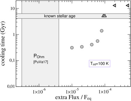
Assuming =100 K requires an extra heating source that maintains such a high heat flux
at present times. For inflated hot Jupiters, extra heating of 0.1% to a few percent of the
incident stellar irradiation is required to explain their large radius, which is consistent with Ohmic heating
(Thorngren & Fortney, 2018).
For Men c, less extra heating is required
(0.01; gray dashed curve). However, the mechanism that may provide this extra heating to
the smaller Men c is not obvious.
While Ohmic heating may occur at sub-Neptunes (Pu & Valencia, 2017),
the predicted amount falls short by two orders of magnitude of what is needed for Men c
(Figure 8, top right).
Another option is tidal heating provided that the planet is on an eccentric orbit, although
the orbital eccentricity remains poorly constrained
(Gandolfi et al., 2018; Huang et al., 2018; Damasso et al., 2020).
For an eccentricity = and tidal quality factor 103 we find
that tidal heating affects negligibly the planetary cooling.
Tidal heating however becomes effective at extending the cooling time of an atmosphere with
=100 K up to the current system’s age if, for example, =0.02 and
103 (about three times the Earth’s tidal quality factor),
or if =0.1 and 5104 (about the Saturn/Uranus/Neptune value).
Further, we estimated the circularization time for these two configurations
(Jackson et al., 2008) to be =0.6 and 30 Gyr respectively.
Even the shortest of them is on the order of our prescribed survival time. It is thus
reasonable to expect that the recent history of Men c’s atmosphere may have occurred
while the planet followed an eccentric orbit that could have sustained 100 K.
It is also conceivable that the outer companion in the Men planetary system may
endow a non-negligible eccentricity to the innermost planet’s orbit
(De Rosa et al., 2020; Kunovac Hodžić et al., 2020; Xuan & Wyatt, 2020), as is found in some
close-in sub-Neptune-plus-cold Jupiter systems.
Importantly, to the effects of planet mass loss,
higher values that imply
lower are less likely to survive over time scales of Gigayears, which sets
a limit to how high can be given that Men c still hosts an atmosphere.
Finally, we adopt =100 K as a reasonable upper limit for Men c.
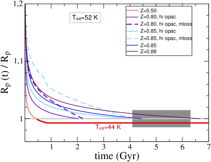
Figure 8 (bottom left) shows evolution tracks for from 0.5 to 0.88
at present-day =52 K. The lower the adopted , the less massive the atmosphere is
and the quicker it cools down and contracts.
Eventually, the planet adopts a state of (nearly) equilibrium evolution with the incident flux, where contraction
slows down and further cooling progresses on very long timescales.
In this state, the planet radiates ((100/1150)4610-5)
only 0.006% more than if it was in true equilibrium with the stellar irradiation.
Mass fractions 0.5 may be possible for present 44 K.
For comparison, Saturn has 77 K and Neptune 53 K, and thus we
do not expect that at Men c will be much higher than for them
given that its mass is much lower.
Also, a non-zero eccentricity may keep above such values.
Mass loss, fixed in the preparation of Figure 8 (bottom left) to
21010 g/s, prolongs the cooling time immediately after formation
but speeds up the contraction well into the future as the planet loses its envelope.
We have simulated the future evolution of Men c for some of the compositions
deemed realistic for present-day Men c with the goal of exploring whether the planet
will ever cross the radius valley.
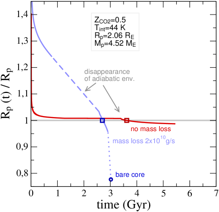
As an example, Figure 8 (bottom right) shows that for (CO2)=0.50 and
=44 K, Men c will turn into a bare rocky core in about 0.5 Gyr.
The same conclusion is found for other – combinations.
The interior structure model calculates the atmospheric pressure-temperature (–) profile using an analytical formulation (Guillot, 2010) that depends on the ratio =/ of constant visible and IR opacities in the –optical depth relation and on the local opacity. For the IR opacities, we take the Rosseland mean for solar composition (Freedman et al., 2008) as our baseline. In our opacity 1 setting, we adopt =0.123 and =1 (bracket denotes average over wavelength) which was confirmed to reproduce well the – profiles published for the H2/He/H2O atmosphere of K2-18 (Scheucher et al., 2020). As Men c’s atmosphere may also contain large abundances of CO2, our opacity 2 setting adopts =0.500 and =2, which is appropriate for a CO2-dominated atmosphere with some admixture of H2/He. Using two sets of opacities for each interior model calculation is a pragmatic way of bracketing the real opacity of Men c’s atmosphere. In a conservative spirit, our constraints on the planet’s bulk composition from the atmospheric stability argument utilize the opacity setting that results in the lowest .
Caption for Table 2.
Summary of photochemical-hydrodynamic model runs. Columns 2–4 quote the assumed nuclei fractions for H, C and O in the bulk atmosphere. Columns 6–13 quote the adopted vmrs at the bar pressure level for H2, H, He, CO2, CO, C, H2O and O, and 14 quotes the corresponding heavy mass fraction. Column 15 quotes the mass flux of H i atoms at the location of the sonic point, which occurs for all cases within the range /=3.5–4.6. Columns 16–20 quote the mass loss rates of H, He, C and O nuclei, and 21 quotes the net mass loss rate. : For these cases, we specified the vmrs at 1 bar considering that molecules such as H2, H2O and O2 become photochemically unstable before reaching the bar pressure level. We also assume that the 1-bar pressure level occurs at the radial distance 2.06 for the TESS radius of the planet. This neglects the vertical extent of the region between a few mbars and 1 bar, a reasonable approximation for moderate atmospheric temperatures. We impose that at the 1-bar level the temperature coincides with the planet’s (1150 K).
| Case | / | Volume mixing ratio at | (=1) | ||||||||||||||||
|---|---|---|---|---|---|---|---|---|---|---|---|---|---|---|---|---|---|---|---|
| H2 | H | He | CO2 | CO | C | H2O | O | [109gs-1] | [109gs-1] | ||||||||||
| 01 | 9.09(-1) | 3.64(-7) | 3.64(-6) | 0.1 | 8.3(-1) | 0.0 | 1.7(-1) | 0.0 | 6.7(-7) | 0.0 | 6.0(-6) | 0.0 | 5.2(-5) | 4.4 | 6.9 | 2.7 | 3.0(-5) | 4.1(-4) | 9.6 |
| 02 | 9.09(-1) | 3.64(-6) | 3.64(-5) | 0.1 | 8.3(-1) | 0.0 | 1.7(-1) | 0.0 | 6.7(-6) | 0.0 | 6.0(-5) | 0.0 | 5.2(-4) | 6.7 | 9.7 | 3.8 | 4.3(-4) | 5.9(-3) | 13.5 |
| 03 | 9.09(-1) | 3.64(-5) | 3.64(-4) | 0.1 | 8.3(-1) | 0.0 | 1.7(-1) | 0.0 | 6.7(-5) | 0.0 | 6.0(-4) | 0.0 | 5.2(-3) | 11.9 | 15.0 | 5.9 | 6.9(-3) | 9.3(-2) | 21.0 |
| 04 | 9.06(-1) | 3.64(-4) | 3.64(-3) | 0.1 | 8.3(-1) | 0.0 | 1.7(-1) | 0.0 | 6.7(-4) | 0.0 | 6.0(-3) | 0.0 | 5.2(-2) | 15.3 | 18.9 | 7.3 | 8.5(-2) | 1.3 | 27.4 |
| 05 | 8.73(-1) | 3.64(-3) | 3.64(-2) | 0.1 | 0.0 | 8.8(-1) | 8.8(-2) | 3.7(-3) | 0.0 | 0.0 | 0.0 | 2.9(-2) | 3.7(-1) | 8.4 | 11.5 | 4.5 | 5.9(-1) | 7.5 | 24.1 |
| 06 | 5.45(-1) | 3.64(-2) | 3.64(-1) | 0.1 | 0.0 | 5.9(-1) | 5.9(-2) | 3.9(-2) | 0.0 | 0.0 | 0.0 | 3.1(-1) | 9.7(-1) | 0.35 | 1.4 | 4.8(-1) | 8.2(-1) | 11.7 | 14.4 |
| 07 | 9.09(-1) | 1.33(-6) | 2.67(-6) | 0.5 | 8.3(-1) | 0.0 | 1.7(-1) | 0.0 | 2.4(-6) | 0.0 | 2.4(-6) | 0.0 | 4.8(-5) | 4.4 | 6.8 | 2.7 | 1.1(-4) | 2.9(-4) | 9.5 |
| 08 | 9.09(-1) | 1.33(-5) | 2.67(-5) | 0.5 | 8.3(-1) | 0.0 | 1.7(-1) | 0.0 | 2.4(-5) | 0.0 | 2.4(-5) | 0.0 | 4.8(-4) | 5.6 | 8.3 | 3.3 | 1.4(-3) | 3.6(-3) | 11.6 |
| 09 | 9.09(-1) | 1.33(-4) | 2.67(-4) | 0.5 | 8.3(-1) | 0.0 | 1.7(-1) | 0.0 | 2.4(-4) | 0.0 | 2.4(-4) | 0.0 | 4.8(-3) | 11.6 | 14.9 | 5.9 | 2.5(-2) | 6.7(-2) | 20.9 |
| 10 | 9.06(-1) | 1.33(-3) | 2.67(-3) | 0.5 | 8.3(-1) | 0.0 | 1.7(-1) | 0.0 | 2.4(-3) | 0.0 | 2.4(-3) | 0.0 | 4.6(-2) | 12.8 | 15.9 | 6.2 | 2.7(-1) | 7.1(-1) | 23.2 |
| 11 | 8.73(-1) | 1.33(-2) | 2.67(-2) | 0.5 | 8.1(-1) | 0.0 | 1.6(-1) | 2.5(-2) | 0.0 | 0.0 | 0.0 | 0.0 | 3.4(-1) | 9.3 | 12.5 | 4.5 | 1.9 | 5.4 | 23.3 |
| 12 | 5.45(-1) | 1.33(-1) | 2.67(-1) | 0.5 | 0.0 | 7.4(-1) | 7.4(-2) | 1.8(-1) | 0.0 | 0.0 | 0.0 | 0.0 | 9.0(-1) | 0.54 | 1.7 | 5.7(-1) | 3.5 | 9.3 | 14.6 |
| 13 | 9.09(-1) | 2.00(-6) | 2.00(-6) | 1 | 8.3(-1) | 0.0 | 1.7(-1) | 0.0 | 3.7(-6) | 0.0 | 0.0 | 0.0 | 4.4(-5) | 4.4 | 6.8 | 2.7 | 1.7(-4) | 2.2(-4) | 9.5 |
| 14 | 9.09(-1) | 2.00(-5) | 2.00(-5) | 1 | 8.3(-1) | 0.0 | 1.7(-1) | 0.0 | 3.7(-5) | 0.0 | 0.0 | 0.0 | 4.4(-4) | 4.8 | 7.3 | 2.8 | 1.8(-3) | 2.3(-3) | 10.1 |
| 15 | 9.09(-1) | 2.00(-4) | 2.00(-4) | 1 | 8.3(-1) | 0.0 | 1.7(-1) | 0.0 | 3.7(-4) | 0.0 | 0.0 | 0.0 | 4.4(-3) | 9.0 | 12.3 | 4.8 | 3.1(-2) | 4.1(-2) | 17.2 |
| 16 | 9.05(-1) | 2.00(-3) | 2.00(-3) | 1 | 8.3(-1) | 0.0 | 1.7(-1) | 0.0 | 3.7(-3) | 0.0 | 0.0 | 0.0 | 4.2(-2) | 10.7 | 13.3 | 5.3 | 3.4(-1) | 4.5(-1) | 19.4 |
| 17 | 8.73(-1) | 2.00(-2) | 2.00(-2) | 1 | 8.0(-1) | 0.0 | 1.6(-1) | 0.0 | 3.7(-2) | 0.0 | 0.0 | 0.0 | 3.1(-1) | 4.9 | 6.8 | 2.6 | 1.7 | 2.3 | 13.4 |
| 18 | 5.45(-1) | 2.00(-1) | 2.00(-1) | 1 | 5.2(-1) | 0.0 | 1.0(-1) | 0.0 | 3.8(-1) | 0.0 | 0.0 | 0.0 | 8.8(-1) | 0.45 | 1.3 | 0.4 | 3.7 | 4.9 | 10.3 |
| 19 | 9.09(-1) | 2.67(-6) | 1.33(-6) | 2 | 8.3(-1) | 0.0 | 1.7(-1) | 0.0 | 2.4(-6) | 2.4(-6) | 0.0 | 0.0 | 4.2(-5) | 4.7 | 7.3 | 2.9 | 2.4(-4) | 1.6(-4) | 10.2 |
| 20 | 9.09(-1) | 2.67(-5) | 1.33(-5) | 2 | 8.3(-1) | 0.0 | 1.7(-1) | 0.0 | 2.4(-5) | 2.4(-5) | 0.0 | 0.0 | 4.2(-4) | 4.6 | 7.1 | 2.8 | 2.3(-3) | 1.5(-3) | 9.9 |
| 21 | 9.09(-1) | 2.67(-4) | 1.33(-4) | 2 | 8.3(-1) | 0.0 | 1.7(-1) | 0.0 | 2.4(-4) | 2.4(-4) | 0.0 | 0.0 | 4.2(-3) | 4.7 | 7.2 | 2.8 | 2.4(-2) | 1.5(-2) | 10.0 |
| 22 | 9.05(-1) | 2.67(-3) | 1.33(-3) | 2 | 8.3(-1) | 0.0 | 1.7(-1) | 0.0 | 2.4(-3) | 2.4(-3) | 0.0 | 0.0 | 4.0(-2) | 5.2 | 7.2 | 2.8 | 2.4(-1) | 1.5(-1) | 10.4 |
| 23 | 8.73(-1) | 2.67(-2) | 1.33(-2) | 2 | 7.9(-1) | 0.0 | 1.6(-1) | 0.0 | 2.4(-2) | 2.4(-2) | 0.0 | 0.0 | 3.0(-1) | 4.4 | 5.4 | 2.1 | 1.8 | 1.2 | 10.5 |
| 24 | 5.45(-1) | 2.67(-1) | 1.33(-1) | 2 | 4.6(-1) | 0.0 | 9.2(-2) | 0.0 | 2.2(-1) | 2.2(-1) | 0.0 | 0.0 | 8.7(-1) | 0.48 | 1.3 | 0.5 | 6.1 | 3.9 | 11.8 |
| 25 | 9.09(-1) | 3.64(-6) | 3.64(-7) | 10 | 8.3(-1) | 0.0 | 1.7(-1) | 0.0 | 6.7(-7) | 6.0(-6) | 0.0 | 0.0 | 3.9(-5) | 4.8 | 7.5 | 2.9 | 3.4(-4) | 4.4(-5) | 10.4 |
| 26 | 9.09(-1) | 3.64(-5) | 3.64(-6) | 10 | 8.3(-1) | 0.0 | 1.7(-1) | 0.0 | 6.7(-6) | 6.0(-5) | 0.0 | 0.0 | 3.9(-4) | 4.8 | 7.5 | 3.0 | 3.4(-3) | 4.4(-4) | 10.5 |
| 27 | 9.09(-1) | 3.64(-4) | 3.64(-5) | 10 | 8.3(-1) | 0.0 | 1.7(-1) | 0.0 | 6.7(-5) | 6.0(-4) | 0.0 | 0.0 | 3.9(-3) | 5.0 | 7.8 | 3.1 | 3.6(-2) | 4.6(-3) | 10.9 |
| 28 | 9.05(-1) | 3.64(-3) | 3.64(-4) | 10 | 8.3(-1) | 0.0 | 1.7(-1) | 0.0 | 6.7(-4) | 6.0(-3) | 0.0 | 0.0 | 3.7(-2) | 5.3 | 7.9 | 3.1 | 3.7(-1) | 4.7(-2) | 11.4 |
| 29 | 8.73(-1) | 3.64(-2) | 3.64(-3) | 10 | 7.8(-1) | 0.0 | 1.6(-1) | 0.0 | 6.5(-3) | 5.8(-2) | 0.0 | 0.0 | 2.9(-1) | 5.1 | 6.6 | 2.6 | 3.1 | 4.0(-1) | 12.7 |
| 30 | 5.46(-1) | 3.64(-1) | 3.64(-2) | 10 | 3.9(-1) | 0.0 | 7.9(-2) | 0.0 | 5.3(-2) | 4.7(-1) | 0.0 | 0.0 | 8.7(-1) | 0.67 | 1.5 | 5.9(-1) | 11.1 | 1.4 | 14.6 |
Caption for Figure 8.
Top Left. Temporal evolution of planet radius () scaled by the measured =2.06 for models with (CO2)=0.85 and present-day values as labeled. Both and decrease with time as the planet cools. The gray box indicates the uncertainty in present radius (0.03) and stellar age (5.21.1 Gyr). For the gray dashed curve of K, the evolution calculations include an extra energy source that converts 0.01% of the incident energy flux into heating of the interior. Top Right. Cooling time, defined as the time to reach the measured planet radius . Symbols are placed at 5.1 Gyr (13 Gyr) if contraction is halted, i.e. if becomes independent of time and agrees with (remains larger than) the measured . All runs are for interior models with =100 K, =0.85, and no mass loss. Bottom Left. Same as top left panel but for models with a lower =52 K and values as labeled. The moderate =0.50 model seems to fall short in cooling time. However, evolving that model further to =44 K leads to equilibrium evolution and (t) still in agreement with the measured value. Bottom Right. Planet size evolution considering a fiducial mass loss of 21010 g s-1 (blue) and omitting mass loss (red) for (CO2)=0.5 and =44 K. Equilibrium is reached when mass loss is omitted. When mass loss is taken into account, the planet continues shrinking as it sheds its atmosphere until it turns into a bare rocky core, which is predicted to happen within 0.5 Gyr from now. The squares indicate potential present states of Men c, from where the evolution is calculated backward and forward in time.
References
- Batalha (2014) Batalha, N.M. 2014. PNAS, 111, 12647
- Barragán et al. (2019) Barragán, O., Gandolfi, D. & Antoniciello, G. 2019. Monthly Notices of the Royal Astronomical Society, Volume 482, Issue 1, p.1017-1030.
- Benneke & Seager (2012) Benneke, B. & Seager, S. 2012. Astrophys. J., 753:100
- Benneke et al. (2019) Benneke, B., Wong, I., Piaulet, C., Knutson, H.A., Lothringer, J., et al. 2019. Astrophys. J. Lett., 887:L14
- Ben-Jaffel & Ballester (2013) Ben-Jaffel, L. & Ballester, G.E. 2013. Astron. & Astrophys., 553:A52
- Ben-Jaffel & Sona Hosseini (2010) Ben-Jaffel, L. & Sona Hosseini, S. 2010. The Astrophysical Journal, Volume 709, Issue 2, pp. 1284-1296.
- Bourrier et al. (2018b) Bourrier, V., Lecavelier des Etangs, A., Ehrenreich, D., Sanz-Forcada, J., Allart, R., et al. 2018. A&A, 620:A147
- Bourrier et al. (2018a) Bourrier, V., Ehrenreich, D., Lecavelier des Etangs, A., Louden, T., Wheatley, P.J., et al. 2018. A&A, 615:A117
- Damasso et al. (2020) Damasso, M., Sozzetti, A., Lovis, C. Barros, S.C.C., Sousa, S.G. et al. 2020. Astronomy & Astrophysics, Volume 642, id.A31, 14 pp.
- De Rosa et al. (2020) De Rosa, R.J., Dawson, R. & Nielsen, E.L. 2020. Astronomy & Astrophysics, Volume 640, id.A73, 13 pp.
- Ehrenreich et al. (2015) Ehrenreich, D., Bourrier, V., Wheatley, P.J., Lecavelier des Etangs, A., Hébrard, G. 2015. Nature, 522:459
- Fortney et al. (2013) Fortney, J.J., Mordasini, C., Nettelmann, N., Kempton, E. M.-R., Greene, T.P. & Zahnle, K., 2013. Astrophys. J., 775:80
- Fossati et al. (2010) Fossati, L., Haswell, C.A., Froning, C.S., Hebb, L., Holmes, S., et al. 2010. Astrophys. J. Lett., 714:L222
- Fulton et al. (2017) Fulton, B.J., Petigura, E.A., Howard, A.W., Isaacson, H., Marcy, G.W. et al. 2017. Astron. J., 154:109
- Freedman et al. (2008) Freedman, R.S., Marley, M.S. & Lodders, K. 2008. The Astrophysical Journal Supplement Series, Volume 174, Issue 2, pp. 504-513 (2008).
- Frisch & Slavin (2003) Frisch, P.C. & Slavin, J.D. 2003. Astrophys. J., 594:844
- Gandolfi et al. (2018) Gandolfi, D., Barragán, O., Livingston, J. H., Fridlund, M., Justesen, A. B., et al., 2018. A&A Letters, 619, L10
- García Muñoz et al. (2020) García Muñoz, A., Youngblood, A., Fossati, L., Gandolfi, D., Cabrera, J. & Rauer, H. 2020. Astrophys. J. Lett., 888:L21
- Gordiets et al. (1982) Gordiets, B.F., Kulikov, Y.N., Markov, M.N. & Marov, M.Y. 1982. J. Geophys. Res., 87:4504
- Guo et al. (2020) Guo, X., Crossfield, I.J.M., Dragomir, D., Kosiarek, M.R., Lothringer, J. et al. 2020. Astronom. J., 159:239
- Guillot (2010) Guillot, T. 2010. Astronomy & Astrophysics, Volume 520, id.A27, 13 pp.
- Hatzes & Rauer (2015) Hatzes, A.P. & Rauer, H. 2015. The Astrophysical Journal Letters, Volume 810, Issue 2, article id. L25.
- Holmström et al. (2008) Holmström, M., Ekenbäck, A., Selsis, F., Penz, T., Lammer, H. & Wurz, P. 2008. Nature, Volume 451, Issue 7181, pp. 970-972 (2008).
- Huang et al. (2018) Huang, C.X., Burt, J., Vanderburg, A., Günther, M.N., Shporer, A. et al. 2018. Astrophys. J. Lett., 868:L39
- Jackson et al. (2008) Jackson, B., Greenberg, R. & Barnes, R. 2008. Astrophys. J., 678:1396-1406.
- King et al. (2019) King, G.W., Wheatley, P.J., Bourrier, V. & Ehrenreich, D. 2019. MNRAS, 484, L49
- Kunovac Hodžić et al. (2020) Kunovac Hodžić, V., Triaud, A.H.M.J., Cegla, H.M. & Chaplin, W.J. 2020. arXiv:2007.06410v1.
- Linsky et al. (2010) Linsky, J.L., Yang, H., France, K., Froning, C.S., Green, J.C., Stocke, J.T. & Osterman, S.N. 2010. Astrophys. J., 717:1291
- Madhusudhan et al. (2020) Madhusudhan, N., Nixon, M.C., Welbanks, L., Piette, A.A.A. & Booth, R.A. 2020. Astrophys. J. Lett., 891:L7
- Mordasini et al. (2015) Mordasini, C., Mollière, P., Dittkrist, K.-M., Jin, S. & Alibert, Y. 2015. Int. J. Astrob., 14:201
- Moses et al. (2013) Moses, J.I., Line, M.R., Visscher, C., Richardson, M.R., Nettelmann, N., et al. 2013. Astrophys. J., 777:34
- Hu & Seager (2014) Hu, R. & Seager, S. 2014. Astrophys. J., 784:63
- Nettelmann et al. (2011) Nettelmann, N., Fortney, J.J., Kramm, U. & Redmer, R. 2011. Astrophys. J., 733:2
- Otegi et al. (2020) Otegi, J.F., Bouchy, F. & Helled, R. 2020. A&A, 634, A43
- Owen & Wu (2013) Owen, J.E. & Wu, Y. 2013. Astrophys. J., 775:105
- Tremblin & Chiang (2013) Tremblin, P. & Chiang, E. 2013. MNRAS, 428:2565
- Poser et al. (2019) Poser, A.J., Nettelmann, N. & Redmer, R. 2019. Atmosphere, 10:664
- Pu & Valencia (2017) Pu, B. & Valencia, D. 2017. The Astrophysical Journal, Volume 846, Issue 1, article id. 47, 12 pp.
- Rogers & Seager (2010) Rogers, L.A. & Seager, S. 2010. Astrophys. J., 716:1208
- Rogers (2015) Rogers, L.A. 2015. Astrophys. J., 801:41
- Scheucher et al. (2020) Scheucher, M., Wunderlich, F., Grenfell, J.L., Godolt, M., Schreier, F., et al. 2020. The Astrophysical Journal, Volume 898, Issue 1, id.44
- Seager et al. (2007) Seager, S., Kuchner, M., Hier-Majumder, C.A. & Militzer, B. 2007. Astrophys. J., 669:1279-1297
- Shaikhislamov et al. (2020a) Shaikhislamov, I.F., Khodachenko, M.L., Lammer, H., Berezutsky, A.G., Miroshnichenko, I.B. & Rumenskikh, M.S. 2020. MNRAS, 491:3435
- Shaikhislamov et al. (2020b) Shaikhislamov, I.F., Fossati, L., Khodachenko, M.L., Lammer, H., García Muñoz, A., Youngblood, A., Dwivedi, N.K. & Rumenskikh, M.S. 2020. A&A, 639:A109
- Thorngren & Fortney (2018) Thorngren, D.P. & Fortney, J.J. 2018. The Astronomical Journal, Volume 155, Issue 5, article id. 214, 10 pp. (2018).
- Tsiaras et al. (2019) Tsiaras, A., Waldmann, I.P., Tinetti, G., Tennyson, J. & Yurchenko, S.N. 2019. Nature Astronomy, 3:1086
- Valencia et al. (2010) Valencia, D., Ikoma, M., Guillot, T. & Nettelmann, N. 2010. A&A 516:A20
- Valencia et al. (2013) Valencia, D., Guillot, T., Parmentier, V. & Freedman, R.S. 2013. Astrophys. J., 775:10
- Verner & Yakovlev (1995) Verner, D.A. & Yakovlev, D.G. 1995, A&A Suppl. 109:125
- Vidal-Madjar et al. (2003) Vidal-Madjar, A., Lecavelier des Etangs, A., Désert, J.-M., Ballester, G.E., Ferlet, R., Hébrard, G. & Mayor, M. 2003. Nature, 422, 143
- Vidal-Madjar et al. (2004) Vidal-Madjar, A., Désert, J.-M., Lecavelier des Etangs, A., Hébrard, G., Ballester, G. E., et al. 2004. The Astrophysical Journal, Volume 604, Issue 1, pp. L69-L72.
- Xuan & Wyatt (2020) Xuan, J.W. & Wyatt, M.C. 2020. Monthly Notices of the Royal Astronomical Society, Volume 497, Issue 2, pp.2096-2118.