A GPU-Accelerated Fast Summation Method Based on Barycentric Lagrange Interpolation and Dual Tree Traversal
Abstract
We present the barycentric Lagrange dual tree traversal (BLDTT) fast summation method for particle interactions. The scheme replaces well-separated particle-particle interactions by adaptively chosen particle-cluster, cluster-particle, and cluster-cluster approximations given by barycentric Lagrange interpolation at proxy particles on a Chebyshev grid in each cluster. The BLDTT is kernel-independent and the approximations can be efficiently mapped onto GPUs, where target particles provide an outer level of parallelism and source particles provide an inner level of parallelism. We present an OpenACC GPU implementation of the BLDTT with MPI remote memory access for distributed memory parallelization. The performance of the GPU-accelerated BLDTT is demonstrated for calculations with different problem sizes, particle distributions, geometric domains, and interaction kernels, as well as for unequal target and source particles. Comparison with our earlier particle-cluster barycentric Lagrange treecode (BLTC) demonstrates the superior performance of the BLDTT. In particular, on a single GPU for problem sizes ranging from =1E5 to 1E8, the BLTC has scaling, while the BLDTT has scaling. In addition, MPI strong scaling results are presented for the BLTC and BLDTT using =64E6 particles on up to 32 GPUs.
keywords:
fast summation, barycentric Lagrange interpolation, dual tree traversal, GPUs, MPI remote memory access1 Introduction
Long-range particle interactions are essential in many areas of computational physics, including calculation of electrostatic or gravitational potentials, as well as discrete convolution sums in boundary element methods. In this context consider the potential due to a set of particles,
| (1) |
where is a target particle, is a source particle with strength , and is an interaction kernel; for example, in electrostatics is a charge and is the Coulomb kernel. The cost of evaluating the potentials by direct summation scales like , which is prohibitively expensive for large systems, but several methods are available to reduce the cost. Among these are mesh-based methods in which the particles are projected onto a regular mesh, such as particle-particle/particle-mesh (P3M) [1] and particle-mesh Ewald (PME) [2], and tree-based methods in which the particles are partitioned into clusters with a hierarchical tree structure, such as Appel’s dual tree traversal (DTT) method [3], the Barnes-Hut treecode (TC) [4], and the Greengard-Rokhlin fast multipole method (FMM) [5, 6]. Other related methods for fast summation of particle interactions include panel clustering [7], hierarchical matrices [8], and multilevel summation [9]. The present approach employs features of the DTT, TC, and FMM, and next we outline key details of these methods.
1.1 Tree-based fast summation methods
Tree-based fast summation methods such as the DTT, TC, and FMM can be described as having two phases. In the precompute phase, the particles are partitioned into a hierarchical tree of clusters, and assuming the particle distribution is homogeneous, this phase generally scales like . In the compute phase, well-separated particle-particle interactions are approximated using for example monopole approximations [3, 4] or higher order multipole expansions [5, 10, 11]. Some differences in the compute phase of these methods are noted as follows. The TC traverses the tree for each target particle to identify well-separated particle-cluster pairs, while the DTT traverses two copies of the tree simultaneously to identify well-separated cluster-cluster pairs; both methods use a multipole acceptance criterion (MAC) for this purpose. The FMM passes information from one level to the next, with a uniform definition of the interaction list at each level; an upward pass computes cluster moments, and a downward pass computes potentials using multipole-to-local and local-to-local translations. The compute phase of the TC scales like , while the compute phase of the FMM [5, 6] and DTT [12, 11] scale like . Next we review developments relevant to the present work in more detail, including dual tree traversal methods, kernel-independent methods, and GPU implementations.
1.2 Dual tree traversal methods
The DDT methods employ cluster-cluster approximations. Early work by Appel developed a DTT-style method using monopole approximations [3]. A later algorithm independently developed by Dehnen for stellar dynamics used Taylor approximations [11]. Subsequent large-scale astrophysical simulations implemented parallel DTTs on many-core architectures [13, 14, 15, 16], and the DTT with Taylor approximations has been applied in molecular dynamics simulations of periodic condensed phase systems [17] and for polarizable force fields [18].
1.3 Kernel-independent methods
Tree-based fast summation methods originally relied on analytic series expansions specific to a given kernel . For example, in the case of the Coulomb and Yukawa kernels, multipole expansions were used in the FMM [6, 19], and Cartesian Taylor expansions were used in the TC [20, 21]. Alternative approximations for the Coulomb kernel were introduced involving numerical discretization of the Poisson integral formula [22] and multipole expansions at pseudoparticles [23]. Eventually kernel-independent methods were developed that require only kernel evaluations and are suitable for a large class of kernels. Among these, the kernel-independent FMM (KIFMM) uses equivalent densities defined on proxy surfaces [24], the black-box FMM (bbFMM) uses polynomial interpolation and SVD compression [25], and the barycentric Lagrange treecode (BLTC) uses barycentric Lagrange interpolation [26, 27]. A number of related proxy point methods have recently been developed using skeletonized interpolation [28] and interpolative decomposition [29, 30]. Several of the kernel-independent fast summation methods have been parallelized for multi-core CPU systems [31, 32, 33, 34, 35, 36, 30].
1.4 GPU implementations
Many modern HPC systems rely heavily on graphics processing units (GPUs) for high-throughput arithmetic. The direct sum in Eq. (1) is well suited for GPU computing; this is because the kernel evaluations can be computed concurrently, where the targets provide an outer level of parallelism, while the sources provide an inner level of parallelism. Early GPU implementations of direct summation achieved a 25 speedup over an optimized CPU implementation [37] and a 250 speedup over a portable C implementation [38]. However, these codes still scale like and there is great interest in implementing the sub-quadratic scaling tree-based methods on GPUs, although this is challenging due to the complexity of these methods in comparison with direct summation. In this direction there have been several GPU implementations of the TC and FMM [39, 40, 41, 42, 36, 43, 44, 45, 46, 47], but we know of only a few GPU implementations of the DTT [48, 49].
1.5 Present work
The present work contributes a GPU-accelerated tree-based fast summation method called barycentric Lagrange dual tree traversal (BLDTT). The BLDTT employs several techniques from previous tree-based methods, including (1) the DTT algorithmic structure [3, 11], (2) barycentric Lagrange interpolation [26, 27, 47], and (3) upward and downward passes similar to those in the FMM, but adapted to the context of barycentric Lagrange interpolation. The BLDTT has several additional features that should be noted. The algorithm replaces well-separated particle-particle interactions by adaptively chosen particle-cluster, cluster-particle, and cluster-cluster approximations, where the clusters are represented by proxy particles at Chebyshev grid points. The approximations are done with barycentric Lagrange interpolation and require only kernel evaluations, hence the BLDTT is kernel-independent. Similar to other tree-based fast summation methods, the BLDTT has a precompute phase and a compute phase; the precompute phase scales like with a small prefactor, while the compute phase scales like , so the observed scaling of the BLDTT is essentially .
As will be shown, the barycentric Lagrange approximations resemble the direct sum in Eq. (1) and they can be efficiently mapped onto GPUs. Based on this observation we present an OpenACC GPU implementation of the BLDTT with MPI remote memory access for distributed memory parallelization. The performance of the BLDTT is documented for calculations with different problem sizes, particle distributions, geometric domains, and interaction kernels, unequal target and source particles. Comparison with our earlier particle-cluster barycentric Lagrange treecode (BLTC) shows the superior performance of the BLDTT. In particular, on a single GPU for problem sizes ranging from =1E5 to 1E8, the BLTC has scaling, while the BLDTT has scaling. In addition, MPI strong scaling results are presented for the BLTC and BLDTT using =64E6 particles on up to 32 GPUs. The BLDTT code is part of the BaryTree library for fast summation of particle interactions available on GitHub [50].
The remainder of the paper is organized as follows. Section 2 describes the barycentric Lagrange dual tree traversal (BLDTT) fast summation method. Section 3 describes our implementation of the BLDTT using MPI remote memory access for distributed memory parallelization and OpenACC for GPU acceleration. Section 4 presents numerical results for several test cases. Section 5 gives the conclusions.
2 Description of BLDTT fast summation method
2.1 Barycentric Lagrange interpolation
We briefly review the barycentric Lagrange form of polynomial interpolation in 1d [26]. Given a function and points , the Lagrange form of the interpolating polynomial is
| (2) |
where the Lagrange polynomial in barycentric form is
| (3) |
This work employs Chebyshev points of the second kind,
| (4) |
in which case the interpolation weights are given by
| (5) |
where if or , and otherwise [51, 26]. The algorithms described below use barycentric Lagrange interpolation in 3D rectangular boxes with interpolation points given by a Cartesian tensor product grid of Chebyshev points adapted to the box. Depending on the context, the interpolation points may also be referred to as proxy particles.
2.2 Algorithm overview
The BLDTT fast summation method computes the potential at a set of target particles due to interactions with a set of source particles; Eq. (1) is a special case in which the targets and sources refer to the same set of particles. First, two hierarchical trees of particle clusters are built, one for the target particles and one for the source particles, where each cluster is a rectangular box; clusters in the target tree are denoted and clusters in the source tree are denoted . The computed potential at a target particle has contributions from four types of interactions as determined by the dual tree traversal algorithm described below. The four types are direct particle-particle (PP) interactions of nearby particles, and particle-cluster (PC), cluster-particle (CP), and cluster-cluster (CC) approximations of well-separated clusters.
Algorithm 1 is a high-level overview of the BLDTT. Lines 1-4 describe the input consisting of target and source particle data, interpolation degree , MAC parameter , and the maximum number of particles in the leaves of each tree, . Line 5 describes the output potentials. Line 6 builds the target tree and source tree containing target clusters and source clusters . Line 7 is the upward pass to compute proxy charges at proxy particles in source clusters . Line 8 is the dual tree traversal to compute interactions. Line 9 is the downward pass to interpolate potentials from proxy particles to target particles in target clusters . The steps will be described in detail below. We summarize the notation used in presenting the BLDTT in Table 1.
| Symbol | Description | Symbol | Description | |
|---|---|---|---|---|
| number of target, source particles | interaction kernel | |||
| target particle in 3D, 1D | potential at target | |||
| source particle in 3D, 1D | PP potential at target in | |||
| source charge of | due to sources in | |||
| target cluster, source cluster | PC potential at target in | |||
| target proxy particle in 3D, 1D | due to proxy sources in | |||
| source proxy particle in 3D, 1D | CP proxy potential at proxy target | |||
| proxy charge of | in due to sources in | |||
| proxy particles in target cluster, | CC proxy potential at proxy target | |||
| source cluster | in due to proxy sources in |
2.3 Tree building
The target and source trees are constructed by the same routines, described here for the target tree. The maximum number of particles per leaf is a user-specified parameter, for the target tree and for the source tree. The root cluster is the minimal bounding box containing all target particles. The root is recursively divided into child clusters, terminating when a cluster contains fewer than particles. Division occurs at the midpoint of the cluster; in general the cluster is bisected in all three coordinate directions, resulting in eight child clusters, with two exceptions. First, a cluster is divided into only two or four children in order to maintain a good aspect ratio, that is, a ratio of longest to shortest side lengths no greater than . Second, a cluster is divided into only two or four children to avoid creating leaf clusters with fewer than particles on average; in particular, if a cluster contains between and particles, it is divided into two children, and if it contains between and particles, it is divided into four children. Upon creation, each cluster is shrunk to the minimal bounding box containing its particles, and a tensor product grid of Chebyshev points adapted to the box is created; these are also referred to as proxy particles. After building the trees, the BLDTT performs the upward pass, dual tree traversal, and downward pass, but before discussing these steps, the next subsection describes the four types of interactions which are eventually combined to compute potentials.
2.4 Four types of interactions
Figure 1 depicts the four types of interactions between a target cluster (left, blue) and a source cluster (right, red), where dots are target/source particles , and crosses are target/source proxy particles . Also shown are the target/source cluster radii , and the target-source cluster distance . These diagrams depict 2D versions of the interactions; in practice the particles are distributed in 3D and the clusters are rectangular boxes. In general, clusters can interact via their particles (dots) or their proxy particles (crosses). Figure 1 shows the four cases: (a) and use particles (PP), (b) uses particles and uses proxy particles (PC), (c) uses proxy particles and uses particles (CP), (d) and both use proxy particles (CC). The interactions are described in detail below; to simplify notation we present the interactions in 1D and note that the extension to 3D is straightforward using tensor products.

|

|
| (a) particle-particle (PP) | (b) particle-cluster (PC) |

|

|
| (c) cluster-particle (CP) | (d) cluster-cluster (CC) |
Particle-particle interaction. Figure 1a depicts a PP interaction. In this case the PP potential at a target particle due to direct interaction with the source particles is denoted by
| (6) |
Particle-cluster approximation. Figure 1b depicts a PC interaction. The kernel is approximated by holding fixed and interpolating with respect to at the proxy particles in ,
| (7) |
Substituting into the particle-particle interaction and rearranging terms yields the PC potential,
| (8) |
where the proxy charges of the proxy particles are
| (9) |
Equation (8) uses to indicate that the target particles interact with the proxy source particles .
Cluster-particle approximation. Figure 1c depicts a CP interaction. The kernel is approximated by interpolating with respect to at the proxy particles in and holding fixed,
| (10) |
Substituting into the particle-particle interaction and rearranging terms yields the CP potential,
| (11) |
where the CP proxy potential is
| (12) |
Equation (11) and Eq. (12) use to indicate that the proxy target particles of interact with the source particles . Equation (11) interpolates from the proxy target particles to the target particles .
Cluster-cluster interaction. Figure 1d depicts a CC interaction. The kernel is interpolated with respect to at the proxy particles in and with respect to at the proxy particles in ,
| (13) |
Substituting into the particle-particle interaction and rearranging terms yields the CC potential,
| (14) |
where the CC proxy potential is
| (15) |
and the proxy charges were defined in Eq. (9). Equation (14) and Eq. (15) use to indicate that the proxy target particles interact with the proxy source particles . Equation (14) interpolates from the proxy target particles to the target particles .
The following three subsections describe the rest of Algorithm 1, comprising the upward pass, dual tree traversal, and downward pass.
2.5 Upward pass
The upward pass computes the proxy charges defined in Eq. (9) for the proxy particles in each source cluster in the source tree, as required in the PC and CC approximations in Eqs. (8) and (15). Note that each source particle contributes to the proxy charges of exactly one cluster at a given level of the tree. Hence with source particles and tree depth , computing the proxy charges directly by Eq. (9) requires operations.
The BLDTT algorithm uses an alternative approach as follows. Let denote a parent cluster with Lagrange polynomials and interpolation points , and let denote the eight child clusters with Lagrange polynomials and interpolation points . As an alternative to Eq. (9), the proxy charges of the parent are computed from the proxy charges of the children by the expression
| (16) |
which is derived in B. The derivation uses the definitions of the parent and child proxy charges and the relation
| (17) |
which is a special case of Eq. (2).
The upward pass starts by computing the proxy charges of the leaves of the source tree using Eq. (9) and then ascending to the root by Eq. (16). This is analogous to the upward pass in the FMM [5] where the multipole moments of a parent cluster are obtained from the moments of its children. As with the FMM, computing the proxy charges this way requires operations, which can be seen as follows. Computing the proxy charges for the leaves requires operations; each of the source particles contributes to one leaf, which contains proxy particles (in 3D). Then, evaluating the child-to-parent relation in Eq. (16) for each parent proxy charge requires operations and is independent of the number of source particles. Since there are clusters in the tree, ascending the tree requires an additional operations. Hence the operation count for the BLDTT upward pass is , as it is for the FMM.
2.6 Dual tree traversal
The dual tree traversal determines which pairs of clusters in the target and source trees interact by one of the four options described above (PP, PC, CP, CC). Before the traversal starts, two sets of potentials are initialized to zero, potentials at the target particles and potentials at the proxy target particles. In the course of the traversal, the potentials are incremented due to PP and PC interactions, and the potentials are incremented due to CP and CC interactions. Following the dual tree traversal, the are interpolated to the target particles and combined with the in the downward pass.
The dual tree traversal uses the recursive procedure DTT() described in Algorithm 2, which takes a target cluster and a source cluster as input. Initially the procedure is called for the root clusters of the target and source trees. In what follows, the clusters are considered to be well-separated if , where are the target and source cluster radii and is the center-center distance between the clusters.
If and are well-separated (line 2), then they interact in one of four ways depending on the number of particles they contain relative to the number of proxy particles in a cluster, which is denoted by in 3D. If and are both large (lines 3-4), then the CC proxy potentials are incremented using Eq. (15); else if is large and is small (lines 5-6), then the CP proxy potentials are incremented using Eq. (12); else if is small and is large (lines 7-8), then the PC potentials are incremented using Eq. (8); else and are both small (line 9) and the PP potentials are incremented using Eq. (6).
If and are not well-separated, then the traversal continues as follows. If and are leaves (lines 11-12), then the PP potentials are incremented using Eq. (6). Otherwise if is a leaf, then it interacts recursively with the children of (line 13), while if is a leaf, then it interacts recursively with the children of (line 14). Finally if and are both not leaves, then the smaller cluster interacts recursively with the children of the larger cluster (lines 15-17).
2.7 Downward pass
The downward pass interpolates the proxy potentials to the target particles and increments the potentials . This can be done in two ways as described below.
First note that each target particle is contained in a chain of target clusters,
| (18) |
where the superscript denotes the level in the target tree. The target cluster at level in the chain has Lagrange polynomials and proxy potentials that contribute to ,
| (19) |
where are the proxy particles of , and the indicates that the results are aggregated with the potentials due to PP and PC interactions previously computed in the DTT. In Eq. (19) the inner sum interpolates potential values from the proxy particles to the target particle , and the outer sum accumulates the results from each level in the tree. Computing as indicated in Eq. (19) requires operations; the factor is the number of target particles , the factor is the number of levels in the target tree, and the inner sum requires operations independent of .
Rather than interpolating from the proxy particles directly to the target particle as in Eq. (19), we utilize a recursive alternative. In what follows, is a parent cluster at level and is a child cluster at level . The procedure interpolates the parent proxy potentials to child proxy potentials ,
| (20) |
where the indicates that the results of the parent-to-child interpolation on the right are aggregated with the child proxy potentials due to CP and CC interactions previously computed in the DTT. This procedure starts with the root cluster of the target tree (level ) and descends to the leaves (level ). Upon reaching the leaves, the proxy potentials are interpolated to the target particles and aggregated with the PP and PC potentials previously computed in the DTT,
| (21) |
It should be noted that the expressions for in Eq. (19) and Eq. (21) are equivalent and this is shown in C.
The recursive form of the downward pass described here is similar to the local-to-local step in the FMM, where the local coefficients are shifted and accumulated, and as in that case the operation count is reduced to . In particular, the parent-to-child interpolation in Eq. (20) requires operations (in 3D), independent of the number of target particles , and the tree contains clusters, so interpolation from the root down to the leaves by Eq. (20) requires operations. Then the final interpolation from the leaf proxy particles to the target particles by Eq. (21) requires operations for each target, yielding complexity for the downward pass.
2.8 Description of BLTC
We briefly describe our previous barycentric Lagrange treecode (BLTC) [27, 47] which has an algorithmic structure resembling the Barnes-Hut treecode [4]. Unlike the BLDTT which builds a tree on both the source and target particles, the BLTC builds a tree of clusters on the source particles and a set of batches on the target particles, where the batches correspond to the leaves of a target tree. Once the source tree is built, the BLTC computes the proxy charges for each source cluster directly from the source particles by Eq. (9). The source tree is then traversed for each target batch, starting at the root of the tree and checking whether a given source cluster and target batch are well-separated. If they are well-separated and the source cluster contains more particles than interpolation points, then the cluster and batch interact by the PC approximation in Eq. (8). If they are not well-separated, then the batch interacts with the children of the source cluster. Leaves in the source tree that are not well-separated from a given target batch, and source clusters that are well-separated but contain more interpolation points than particles interact directly with the target batch by the PP interaction in Eq. (6). For target particles and source particles, the BLTC operation count is + , where the first term arises from the computation of the proxy charges and the second term arises from the source tree traversal.
3 BLDTT implementation
The implementation of the BLDTT for multiple GPUs is largely similar to that of our previous BLTC implementation [47], and is available as part of the BaryTree library for fast summation of particle interactions available on GitHub [50]. The code uses OpenACC directives for GPU acceleration and MPI remote memory access for distributed memory parallelization. Tree building, tree traversal, and MPI communication of particles and clusters occur on the CPU, while the upward pass, particle and cluster interaction computations, and downward pass occur on the GPU. We review here several important details of this implementation.
3.1 Computing interaction lists
We decouple dual tree traversal from the computation of the particle interactions. The dual tree traversal is performed on the CPU, creating four interaction lists for each cluster of the target tree, one for each type of interaction. Each list contains the indices of the source clusters that interact with the target cluster by the given interaction type. The interactions are then computed by directly iterating over the interaction lists; this improves the efficiency of GPU calculations because these lists can be iterated over rapidly and GPU compute kernels (described below) can be queued asynchronously.
3.2 MPI distributed memory parallelization
To implement distributed memory parallelization, we use locally essential trees (LET) [52]. Particles are partitioned by recursive coordinate bisection to create compact sub-domains on each MPI rank using Trilinos Zoltan [53, 54]. Each MPI rank constructs the local source tree and local target tree for its particles. The LET of a rank is the union of the rank’s local source tree and all source clusters from remote ranks interacting with its local target tree. Even though constructing the LETs requires an all-to-all communication, the amount of data acquired by each rank grows only logarithmically with the problem size [52]. The construction and communication required by the LETs are performed using MPI passive target synchronization remote memory access (RMA). RMA is a one-sided communication model within MPI in which an origin process can put data onto a target process or get data from a target process through specially declared memory windows, with no active involvement from the target process. This approach enables each rank to construct its LET asynchronously from other ranks.
3.3 GPU details
The GPU implementation uses eight compute kernels, two for the upward pass, four for computing interactions determined by the dual tree traversal, and two for the downward pass. The compute kernels are generated with OpenACC directives, compiled with the PGI C compiler. We utilize asynchronous launch of kernels in multiple GPU streams to hide as much latency as possible. The approach described here generalizes to multiple GPUs in a straightforward manner, in which each GPU corresponds to one MPI rank.
The first upward pass kernel computes the proxy charges for a given leaf in the source tree. For each leaf, this kernel is launched asynchronously, and any further computation is blocked until all leaf proxy charges are computed. The second upward pass kernel computes the proxy charges of a parent cluster using the proxy charges of its children. For a given level of the tree, this kernel is launched asynchronously for each cluster at that level, and any further computation is blocked until all proxy charges at that level are computed. The proxy charges at a given level are computed after the computation of the proxy charges at the previous level is complete.
The four DTT kernels compute the interaction of a target cluster with a source cluster. Each PP, PC, CP, and CC interaction launches one compute kernel. All such kernels are launched asynchronously and further computation is blocked until these kernels complete. The four interaction kernels have a similar structure in which the outer loop is over the target particles or proxy particles in the target cluster, and the inner loop is over the source particles or proxy particles in the source cluster. Importantly, due to the Lagrange form of barycentric interpolation, the inner loop iterations are independent, unlike alternative approximation methods which are sequential. The outer loop is mapped to the gang construct in OpenACC and the inner loop is mapped to the vector construct. Conceptually, a member of a gang corresponds to a thread block, while a member of a vector corresponds to an individual thread.
The two downward pass compute kernels are similar in structure to the upward pass kernels. At each level of the target tree above the leaves, beginning with the root, the first downward pass compute kernel is launched asynchronously for each target cluster at that level to interpolate the proxy potentials of the cluster to its children. Further computation is blocked until all compute kernels at a given level complete. Finally, the second downward pass compute kernel is launched asynchronously for each target leaf to interpolate the proxy potentials to the target particles.
4 Results
We demonstrate the BLDTT on a series of test cases and compare its performance to that of the BLTC. First, we compare the scaling of the BLTC and BLDTT on problem sizes from 1E5 to 1E8 particles. Second, we briefly demonstrate the GPU acceleration of the BLDTT over a CPU implementation. Third, we display the performance of the BLDTT on various particle distributions: random uniform, Gaussian, and Plummer [55, 56]. We also demonstrate the benefit of including CP and PC interactions in the BLDTT algorithm. Fourth, we display the performance of the BLDTT on various geometries: a slab, a slab, and a spherical shell with all particles at radius 1. Fifth, we investigate BLDTT performance in cases where the number of sources and targets are unequal. Sixth, we show performance results for various interaction kernels, including an oscillatory kernel, the Yukawa kernel, and the regularized Coulomb kernel. Last, we show MPI strong scaling performance on 1 to 32 GPUs.
Except for the Plummer distribution runs, the source particle charges are random uniformly distributed on . Except for the runs involving unequal numbers of sources and targets, the source and target particle sets are identical. All computations use the Coulomb interaction kernel except for the examples in section 4.6. All runs used a maximum leaf or batch size of 2000. To facilitate comparison of the BLDTT and BLTC across this wide variety of problems, Figures 4, 5, 8, and 10 all use the same axes to display time vs. error.
The calculations are done in double precision arithmetic and the reported errors are the relative error,
| (22) |
where are the target potentials computed by direct summation and are computed by the BLDTT fast summation method. The error was sampled at a random subset of 0.1% of the target particles in all cases.
The computations were performed on the NVIDIA P100 GPU nodes at the San Diego Supercomputer Center Comet machine, where each node contains four GPUs, and each GPU has 16GB of memory. Except for the MPI strong scaling results in section 4.7, each computation was run on a single GPU. The code was compiled with the PGI C compiler using the -O3 optimization flag. For parallel scaling results, the Zoltan library of Trilinos [53, 54] was used to perform recursive coordinate bisection to load balance the particles. As described in the previous section, tree building and interaction list building are performed on the CPU, while the upward pass, particle interactions, and downward pass are performed on the GPU.
4.1 Problem size scaling
Figure 2 shows the compute time (s) for direct summation (green), BLTC (red), and BLDTT (blue) with =1E5, 1E6, 1E7, 1E8 random uniformly distributed source and target particles in the cube interacting by the Coulomb kernel. The BLTC and BLDTT use MAC parameter and interpolation degree , yielding 7-8 digit accuracy. Figure 2(a) is a linear plot, showing that the BLDTT is about twice as fast as the BLTC, and both are much faster than direct summation. Figure 2(b) is a logarithmic plot with reference lines scaling as (dashed), (dotted), and (dash-dotted), showing that as the problem size increases, the BLTC has asymptotic scaling, while the BLDTT has asymptotic scaling, as expected. Table 2 records the compute time and error; the asymptotic scaling of the compute time can be quantitatively confirmed, and while there is a slight increase in the error with problem size, the BLDTT error is consistently smaller than the BLTC error.

|

|
|---|---|
| (a) linear scale | (b) logarithmic scale |
| BLTC time (s) | BLTC error | BLDTT time (s) | BLDTT error | |
|---|---|---|---|---|
| 1E5 | 2.15E1 | 1.75E8 | 2.19E1 | 1.58E8 |
| 1E6 | 4.71E+0 | 1.42E7 | 3.56E+0 | 3.67E8 |
| 1E7 | 6.81E+1 | 4.68E7 | 4.40E+1 | 4.12E8 |
| 1E8 | 8.96E+2 | 9.23E7 | 4.82E+2 | 4.17E8 |
4.2 GPU acceleration of BLDTT
In this subsection we compare the BLDTT running on a single NVIDIA P100 GPU to running on 8 CPU cores of an Intel Xeon E5-2680v3 processor at 2.50 GHz with MPI parallelization. We perform the same four calculations above, so the errors are the same as those in Table 2. Table 3 gives the compute times, showing that the BLDTT achieves 30-40 speedup on the GPU compared the 8 CPU cores. The efficiency of the BLDTT running on the GPU is due to the independent nature of the terms in the barycentric Lagrange approximation, which allows them to be computed concurrently.
| CPU time (s) | GPU time (s) | speedup | |
|---|---|---|---|
| 1E5 | 7.84E+0 | 2.19E1 | 35.8 |
| 1E6 | 1.45E+2 | 3.56E+0 | 40.7 |
| 1E7 | 1.40E+3 | 4.40E+1 | 31.8 |
| 1E8 | 1.70E+4 | 4.82E+2 | 35.3 |
4.3 Non-uniform particle distributions
We investigate the performance of the BLDTT for three different random particle distributions: (a) uniform particles in , (b) Gaussian particles with radial pdf , (c) Plummer particles [55, 56] with radial pdf and cutoff at in all three Cartesian coordinates. The charges of the uniform and Gaussian particles are uniformly distributed in , while the Plummer particle charges are set to , where is the total number of particles. To give a sense of the structure of the distributions, Figure 3 depicts the three distributions with =4E5 particles. Compared to the uniform case (a), the Gaussian and Plummer distributions (b,c) are more highly concentrated near the origin, with the Gaussian decaying more rapidly away from the origin and the Plummer decaying less rapidly.

|
 |
 |
|---|---|---|
| (a) Random Uniform | (b) Gaussian | (c) Plummer |
Figure 4 shows the compute time (s) versus relative error for the BLDTT (blue, solid) and BLTC (red, dashed) on these three distributions with =2E7 particles. Each connected curve represents constant MAC with (), (), (), and the interpolation degree increases from right to left on each curve. For these parameter choices the errors span the range from 1 digit to 10 digit accuracy. Large is more efficient for low accuracy and small is more efficient for high accuracy. The results show that the BLDTT has consistently better performance than the BLTC and is less sensitive to the particle distribution.

|

|

|
|---|---|---|
| (a) Random Uniform | (b) Gaussian | (c) Plummer |
To demonstrate the effect of including PC and CP interactions in the BLDTT, Figure 5 shows the compute time versus relative error for the BLDTT (blue, solid) as presented in this paper using PP, PC, CP and CC interactions, and a version of the BLDTT (red, dashed) using only CC and PP interactions. When only CC and PP interactions are used, the interaction between a target cluster and a source cluster is handled by PP interaction if either cluster contains more interpolation points than particles, whereas the flexibility to choose PC or CP interactions in those cases improves performance at higher interpolation degree, especially for the non-uniform particle distributions.

|

|

|
|---|---|---|
| (a) random uniform | (b) Gaussian | (c) Plummer |
To further understand the effect of including PC and CP interactions, next we compare the number of pointwise interactions used by the two versions of the BLDTT, where by pointwise interaction we mean one evaluation of the kernel . Results are shown for MAC and interpolation degree , for the same three random distributions with =2E7 particles as above. Figure 6 displays results for the four types of interactions in stacked bars, CC (blue), PP (orange), PC (yellow), CP (purple), from bottom to top, where the left bar in each pair is the BLDTT with CC and PP interactions only, and the right bar is the BLDTT with PP, PC, CP, and CC interactions. In this case a direct sum calculation would use 4E14 PP interactions, while the BLDTT calculations use less than 6E12 interactions. The results show that for high degree, introducing PC and CP interactions into the BLDTT significantly reduces the number of PP interactions, replacing them with a much smaller number of PC and CP interactions, and this effect is more prominent for the nonuniform particle distributions.

|

|

|
|---|---|---|
| (a) Random Uniform, | (b) Gaussian, | (c) Plummer, |
4.4 Non-cubic particle domains
We demonstrate here the performance of the BLDTT on three examples with non-cubic particle domains depicted in Figure 7: (a) thin slab of dimensions , (b) square rod of dimensions , and (c) spherical surface of radius . In all cases the particles are random uniformly distributed.

|

|

|
|---|---|---|
| (a) 2D Slab | (b) 1D Slab | (c) Spherical Shell |
Figure 8 shows the compute time (s) versus the relative error for the BLDTT (blue, solid) and BLTC (red, dashed) on these three examples with =2E7 particles, using MAC and interpolation degree . The results show that the BLDTT has consistently better performance than the BLTC. Compared to the cubic domain results in Figure 4(a), the BLDTT achieves similar levels of error and runs somewhat faster for the non-cubic domains. Heuristically, the BLDTT run time depends on the complexity of the tree; in particular, the tree is an oct-tree for the cubic domain, close to a quad-tree for the thin slab and sphere surface, and close to a binary tree for the square rod. The results indicate that BLDTT automatically adapts to the complexity of the tree without requiring explicit reprogramming.

|

|

|
|---|---|---|
| (a) thin slab | (b) square rod | (c) sphere surface |
4.5 Unequal targets and sources
To demonstrate the performance of the BLDTT with unequal target and source particles, we consider a cluster-particle variant of the BLTC for comparison [57, 58]. The CP-BLTC builds a tree on the targets and a set of batches on the sources, and rather than using PP and PC interactions, it uses PP and CP interactions. Instead of an upward pass to compute proxy charges, the CP-BLTC has an downward pass to interpolate proxy potentials to targets. While the compute phase of the BLTC is , the compute phase of the CP-BLTC is . Since the compute phase is in general the most expensive part of the algorithm, we expect the BLTC to perform better than the CP-BLTC when , and vice versa.
Figure 9 shows the compute time (s) versus relative error for the BLTC (red, dashed), CP-BLTC (green, dash-dotted), and BLDTT (blue, solid) with (a) =2E7 targets, =2E6 sources, (b) =2E6 targets, =2E7 sources, for MAC and interpolation degree as above. For (a) , the CP-BLTC outperforms the BLTC, for (b) , the BLTC outperforms the CP-BLTC for errors below 1E-5, while the BLDTT outperforms the two treecodes in both cases. Note however in (b) that for MAC and error larger than 1E-3, the CP-BLTC runs slightly faster than the BLDTT; this is due to the cost of the upward pass in the BLDTT, which is more expensive than the downward pass, and with low degree , makes up a substantial portion of the compute time. The results demonstrate the ability of the BLDTT to efficiently adapt to the case of unequal targets and sources.

|

|
|---|---|
| (a) E7, E6 | (b) E6, E7 |
4.6 Other interaction kernels
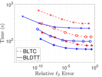
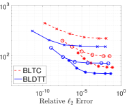
In previous sections we considered particles interacting through the Coulomb potential. Here we demomstrate the performance of the BLDTT on three other interaction kernels: (a) an oscillatory kernel, , (b) a Yukawa kernel, , and (c) a regularized Coulomb kernel, , with . Figure 10 shows the compute time (s) versus relative error for the BLDTT (blue, solid) and BLTC (red, dashed) for these three kernels on =2E7 random uniformly distributed particles in the cube for various values of the MAC and interpolation degree . The results show that the BLDTT has consistently better performance than the BLTC. Comparing with the Coulomb potential resuts in Figure 4(a), we see that the BLDTT has similar performance for the various interaction kernels, reflecting the kernel-independent nature of the method.
|

|
|
|---|---|---|
| (a) | (b) | (b) |
4.7 MPI strong scaling
Finally, we demonstrate the MPI strong scaling of the BLDTT up to 32 NVIDIA P100 GPUs with one MPI rank per GPU. The particles are partitioned into geometrically localized domains by Trilinos Zoltan [53, 54]. Figure 11 depicts a sample domain decomposition for =1.6E6 random uniformly distributed particles in the cube , (a) across 8 ranks with 2E5 particles per rank, and (b) across 16 ranks with 1E5 particles per rank. Colors represent particles residing on different ranks.
 |
 |
| (a) | (b) |
We consider a problem with =64E6 particles using MAC and interpolation degree yielding error 1E-8. Figure 12 shows the compute time versus the number of GPUs for (a) random uniform, (b) Gaussian, and (c) Plummer distributions for the BLDTT (blue) and BLTC (red), where dashed lines indicate ideal scaling and the boxed numbers show the parallel efficiency. As was shown earlier for one GPU in Figure 4, the BLDTT is consistently faster than the BLTC up to 32 GPUs, and the speedup improves for the nonuniform particle distributions. The BLDTT and BLTC have generally similar parallel efficiency for all three distributions; for example on 32 GPUs, the BLDTT has parallel efficiency 77%, 65%, and 66% for the uniform, Gaussian, and Plummer distributions, compared to 83%, 81%, and 64% for the BLTC.

|

|

|
|---|---|---|
| (a) Uniform | (b) Gaussian | (c) Plummer |
The slightly lower parallel efficiency for the BLDTT compared to the BLTC can be explained by the greater efficiency of the BLDTT algorithm itself. Figure 13 shows the component breakdown as a percentage of run time (total wall clock time) of the (a) BLTC and (b) BLDTT for the uniform distribution results in Figure 12(a). The components shown are the upward pass (blue), compute due to local sources and source clusters (orange), compute due to remote sources and source clusters (yellow), downward pass (purple), LET construction and communication (green), and other (light blue), which includes tree building and interaction list building. The breakdown is based on timing results for the most expensive MPI rank in each case. Note that the LET construction accounts for an increasing percentage of the run time as the number of ranks increases. This is to be expected as more particles reside on remote ranks and must be communicated, and this is the primary factor that impedes ideal parallel scaling. The LET construction time is nearly identical for the BLTC and BLDTT, however since the BLDTT computations are more efficient, the LET construction accounts for a larger percentage of the run time and this results in the lower parallel efficiency seen in Figure 12 as the number of ranks increases.

|

|
|---|---|
| (a) BLTC | (b) BLDTT |
5 Conclusion
We presented the barycentric Lagrange dual tree traversal (BLDTT) fast summation method for particle interactions, and its OpenACC implementation with MPI remote memory access for distributed memory parallelization running on multiple GPUs. The BLDTT builds adaptive trees of clusters on the target particles and source particles, where each cluster is the minimal bounding box of its particles, and a parent cluster may have 8, 4, or 2 children. The BLDTT uses a dual tree traversal strategy [3, 11] to determine well-separated target and source clusters that interact through particle-cluster (PC), cluster-particle (CP), or cluster-cluster (CC) approximations based on barycentric Lagrange interpolation at proxy particles defined by tensor product Chebyshev points of the 2nd kind in each cluster [26, 27]. The BLDTT has an upward pass and downward pass similar those in the FMM [5], although it relies on interlevel polynomial interpolation rather than translation of expansion coefficients. The BLDTT is kernel-independent, requiring only kernel evaluations. The distributed memory parallelization of the BLDTT uses recursive coordinate bisection for domain decomposition and MPI remote memory access to build locally essential trees on each rank [52]. The PP, PC, CP, and CC interactions all have a direct sum form that efficiently maps onto the GPU, where target particles provide an outer level of parallelism, and source particles provide an inner level of parallelism. The BLDTT code is part of the BaryTree library for fast summation of particle interactions available on GitHub [50].
The performance of the BLDTT was compared with that of the BLTC, an earlier particle-cluster barycentric Lagrange treecode [27]. For the systems of size =1E5 to =1E8 studied here running on a single GPU, the BLTC scales like , while the BLDTT scales like . The BLDTT was applied to different random particle distributions (uniform, Gaussian, Plummer), different particle domains (thin slab, square rod, spherical surface), unequal sets of target and source particles, and different interaction kernels (oscillatory, Yukawa, singular and regularized Coulomb). The BLDTT had consistently better performance than the BLTC, showing its ability to adapt to different situations. Finally, the MPI strong scaling of the BLDTT and BLTC was demonstrated on up to 32 GPUs for =64E6 particles with 7-8 digit accuracy. Across these simulations the parallel efficiency of both codes is better than 64%, while the BLDTT is 1.5-2.5 faster than the BLTC.
Future work to further improve the efficiency of the BLDTT could investigate overlapping communication and computation, building tree nodes that span multiple ranks, using mixed-precision arithmetic, and employing barycentric Hermite interpolation [59]. We also anticipate applying the BLDTT to speed up integral equation based Poisson–Boltzmann implicit solvent computations [60] and density functional theory calculations [61].
6 Acknowledgements
This work was supported by National Science Foundation grant DMS-1819094, Extreme Science and Engineering Discovery Environment (XSEDE) grants ACI-1548562, ASC-190062, and the Mcubed program and Michigan Institute for Computational Discovery and Engineering (MICDE) at the University of Michigan.
References
- [1] R. W. Hockney, J. W. Eastwood, Computer Simulation Using Particles, Taylor & Francis, 1988.
- [2] U. Essmann, L. Perera, M. Berkowitz, T. Darden, H. Lee, L. Pederson, A smooth particle mesh Ewald method, J. Chem. Phys. 103 (1995) 8577–8593.
- [3] A. W. Appel, An efficient program for many-body simulation, SIAM J. Sci. Stat. Comput. 6 (1) (1985) 85–103.
- [4] J. E. Barnes, P. Hut, A hierarchical force-calculation algorithm, Nature 324 (1986) 446–449.
- [5] L. Greengard, V. Rokhlin, A fast algorithm for particle simulations, J. Comput. Phys. 73 (1987) 325–348.
- [6] H. Cheng, L. Greengard, V. Rokhlin, A fast adaptive multipole algorithm in three dimensions, J. Comput. Phys. 155 (2) (1999) 468–498.
- [7] W. Hackbusch, Z. P. Nowak, On the fast matrix multiplication in the boundary element method by panel clustering, Numer. Math. 54 (1989) 463–491.
- [8] W. Hackbusch, Hierarchical Matrices: Algorithms and Analysis, Spring, 2015.
- [9] D. J. Hardy, Z. Wu, J. C. Phillips, J. E. Stone, R. D. Skeel, K. Schulten, Multilevel summation method for electrostatic force evaluation, J. Chem. Theory Comput. 11 (2015) 766–779.
- [10] K. Lindsay, R. Krasny, A particle method and adaptive treecode for vortex sheet motion in three-dimensional flow, J. Comput. Phys. 172 (2) (2001) 879–907.
- [11] W. Dehnen, A hierarchical force calculation algorithm, J. Comput. Phys. 179 (2002) 27–42.
- [12] K. Esselink, The order of Appel’s algorithm, Inf. Process. Lett. 41 (3) (1992) 141–147.
- [13] K. Taura, J. Nakashima, R. Yokota, N. Maruyama, A task parallel implementation of fast multipole methods, in: 2012 SC Companion: High Performance Computing, Networking Storage and Analysis, 2012, pp. 617–625.
- [14] R. Yokota, An FMM based on dual tree traversal for many-core architectures, J. Algorithm Comput. Technol. 7 (3) (2013) 301–324.
- [15] W. Dehnen, A fast multipole method for stellar dynamics, Comput. Astrophys. Cosmol. 1 (1) (2014) 1–23.
- [16] B. Lange, P. Fortin, Parallel dual tree traversal on multi-core and many-core architectures for astrophysical N-body simulations, Proc. 20th Int. Eur. Conf. Parallel Distrib. Comput. (Euro-Par 2014) (2014) 716–727.
- [17] K. Lorenzen, M. Schwörer, P. Tröster, S. Mates, P. Tavan, Optimizing the accuracy and efficiency of fast hierarchical multipole expansions for MD simulations, J. Chem. Theory Comput. 8 (10) (2012) 3628–3636.
- [18] J. Coles, M. Masella, The fast multipole method and point dipole moment polarizable force fields, J. Chem. Phys. 142 (2) (2015) 024109.
- [19] L. Greengard, J. Huang, A new version of the fast multipole method for screened Coulomb interactions in three dimensions, J. Comput. Phys. 180 (2) (2002) 642 – 658.
- [20] Z.-H. Duan, R. Krasny, An adaptive treecode for computing nonbonded potential energy in classical molecular systems, J. Comput. Chem. 22 (2) (2001) 184–195.
- [21] P. Li, H. Johnston, R. Krasny, A Cartesian treecode for screened Coulomb interactions, J. Comput. Phys. 228 (2009) 3858–3868.
- [22] C. R. Anderson, An implementation of the fast multipole method without multipoles, SIAM J. Sci. Stat. Comput. 13 (1992) 923–947.
- [23] J. Makino, Yet another fast multipole method without multipoles–pseudoparticle multipole method, J. Comput. Phys. 151 (1999) 910–920.
- [24] L. Ying, G. Biros, D. Zorin, A kernel-independent adaptive fast multipole algorithm in two and three dimensions, J. Comput. Phys. 196 (2) (2004) 591–626.
- [25] W. Fong, E. Darve, The black-box fast multipole method, J. Comput. Phys. 228 (23) (2009) 8712–8725.
- [26] J.-P. Berrut, L. N. Trefethen, Barycentric Lagrange interpolation, SIAM Rev. 46 (3) (2004) 501–517.
- [27] L. Wang, R. Krasny, S. Tlupova, A kernel-independent treecode based on barycentric Lagrange interpolation, Commun. Comput. Phys. 28 (2020) 1415–1436.
- [28] L. Cambier, E. Darve, Fast low-rank kernel matrix factorization using skeletonized interpolation, SIAM J. Sci. Comput. 41 (3) (2019) A1652–A1680.
- [29] X. Xing, E. Chow, Interpolative decomposition via proxy points for kernel matrices, SIAM J. Matrix Anal. Appl. 41 (1) (2020) 221–243.
- [30] H. Huang, X. Xing, E. Chow, H2Pack: High-performance matrix package for kernel matrices using the proxy point method, ACM Trans. Math. Softw. (2020).
- [31] L. Ying, G. Biros, D. Zorin, H. Langston, A new parallel kernel-independent fast multipole method, Proc. 2003 ACM/IEEE Conf. Supercomput. (SC03) (2003) 14.
- [32] I. Lashuk, A. Chandramowlishwaran, M. H. Langston, T.-A. Nguyen, R. Sampath, A. Shringarpure, R. Vuduc, L. Ying, D. Zorin, G. Biros, A massively parallel adaptive fast multipole method on heterogeneous architectures, Commun. ACM 55 (2012) 101–109.
- [33] W. B. March, B. Xiao, S. Tharakan, C. D. Yu, G. Biros, A kernel-independent FMM in general dimensions, Proc. Int. Conf. High Perf. Comput. Networking, Storage Anal. (SC15) (2015) 24:1–24:12.
- [34] D. Malhotra, G. Biros, PVFMM: A parallel kernel independent FMM for particle and volume potentials, Commun. Comput. Phys. 18 (3) (2015) 808–830.
- [35] D. Malhotra, G. Biros, Algorithm 967: A distributed-memory fast multipole method for volume potentials, ACM Trans. Math. Softw. 43 (2016) 1–27.
- [36] T. Takahashi, C. Cecka, E. Darve, Optimization of the parallel black-box fast multipole method on CUDA, 2012 Innov. Parallel Comput. (InPar) (2012) 1–14.
- [37] E. Elsen, M. Houston, V. Vishal, E. Darve, P. Hanrahan, V. Pande, N-body simulation on GPUs, Proc. 2006 ACM/IEEE Conf. Supercomput. (SC06) (2006) 188.
- [38] L. Nyland, M. Harris, J. Prins, Fast -body simulation with CUDA, GPU Gems, Vol. 3 (2009) 677–695.
- [39] T. Hamada, T. Narumi, R. Yokota, K. Yasuoka, K. Nitadori, M. Taiji, 42 TFlops hierarchical N-body simulations on GPUs with applications in both astrophysics and turbulence, Proc. Int. Conf. High Perf. Comput. Networking, Storage Anal. (SC09) (2009) 1–12.
- [40] M. Burtscher, K. Pingali, An efficient CUDA implementation of the tree-based Barnes Hut -body algorithm, in: W.-M. Hwu (Ed.), GPU Computing Gems Emerald Edition, Morgan Kaufmann/Elsevier, 2011, Ch. 6, pp. 75–92.
- [41] R. Yokota, L. A. Barba, Comparing the treecode with FMM on GPUs for vortex particle simulations of a leapfrogging vortex ring, Comput. Fluids. 45 (1) (2011) 155–161, 22nd International Conference on Parallel Computational Fluid Dynamics (ParCFD 2010).
- [42] R. Yokota, J. P. Bardhan, M. G. Knepley, L. A. Barba, T. Hamada, Biomolecular electrostatics using a fast multipole BEM on up to 512 GPUs and a billion unknowns, Comput. Phys. Commun. 182 (2011) 1272–1283.
- [43] J. Bédorf, E. Gaburov, S. P. Zwart, A sparse octree gravitational -body code that runs entirely on the GPU processor, J. Comput. Phys. 231 (7) (2012) 2825–2839.
- [44] J. Bédorf, E. Gaburov, M. S. Fujii, K. Nitadori, T. Ishiyama, S. P. Zwart, 24.77 Pflops on a gravitational tree-code to simulate the Milky Way Galaxy with 1860 GPUs, Proc. Int. Conf. High Perf. Comput. Networking, Storage Anal. (SC14) (2014) 54–65.
- [45] W. Boukaram, G. Turkiyyah, D. Keyes, Hierarchical matrix operations on GPUs: Matrix-vector multiplication and compression, ACM Trans. Math. Softw. 45 (1) (2019) 3:1–3:28.
- [46] W. Boukaram, G. Turkiyyah, D. Keyes, Randomized GPU algorithms for the construction of hierarchical matrices from matrix-vector operations, SIAM J. Sci. Comput. 41 (2019) C339–C366.
- [47] N. Vaughn, L. Wilson, R. Krasny, A GPU-accelerated barycentric Lagrange treecode, Proc. 21st IEEE Int. Workshop Parallel Distrib. Sci. Eng. Comput. (PDSEC 2020) (2020).
- [48] R. Yokota, L. A. Barba, Hierarchical -body simulations with autotuning for heterogeneous systems, Comput. Sci. Eng. 14 (2012) 30–39.
- [49] P. Fortin, M. Touche, Dual tree traversal on integrated GPUs for astrophysical N-body simulations, Int. J. High Perform. Comput. Appl. (2019) 1–13.
-
[50]
N. Vaugh, L. Wilson, R. Krasny,
BaryTree (2020).
URL https://github.com/Treecodes/BaryTree - [51] H. E. Salzer, Lagrangian interpolation at the Chebyshev points ; some unnoted advantages, Comput. J. 15 (1972) 156–159.
- [52] M. S. Warren, J. K. Salmon, Astrophysical N-body simulations using hierarchical tree data structures, Proc. 1992 ACM/IEEE Conf. Supercomput. (SC92) (1992) 570–576.
-
[53]
The Zoltan Project Team,
The Zoltan Project (2020).
URL https://trilinos.github.io/zoltan.html - [54] E. G. Boman, U. V. Catalyurek, C. Chevalier, K. D. Devine, The Zoltan and Isorropia parallel toolkits for combinatorial scientific computing: Partitioning, ordering, and coloring, Sci. Program. 20 (2) (2012) 129–150.
- [55] H. C. Plummer, On the problem of distribution in globular star clusters, Mon. Not. R. Astr. Soc. 71 (1911) 460–470.
- [56] H. Dejonghe, A completely analytical family of anisotropic Plummer models, Mon. Not. R. Astr. Soc. 224 (1987) 13–39.
- [57] H. A. Boateng, Cartesian treecode algorithms for electrostatic interactions in molecular dynamics simulations, Ph.D. thesis, University of Michigan (2010).
- [58] H. A. Boateng, R. Krasny, Comparison of treecodes for computing electrostatic potentials in charged particle systems with disjoint targets and sources, J. Comput. Chem. 34 (25) (2013) 2159–2167. doi:10.1002/jcc.23371.
- [59] R. Krasny, L. Wang, A treecode based on barycentric hermite interpolation for electrostatic particle interactions, Comput. Math. Biophys. 7 (2019) 73–84.
- [60] W. Geng, R. Krasny, A treecode-accelerated boundary integral Poisson–Boltzmann solver for electrostatics of solvated biomolecules, J. Comput. Phys. 247 (2013) 62–78.
- [61] N. Vaughn, V. Gavini, R. Krasny, Treecode-accelerated Green iteration for Kohn–Sham density functional theory, arXiv e-prints (2020) arXiv:2003.01833.
Appendix A Preliminaries
The derivation of the upward pass and downward pass rely on a property of interpolating polynomials. For a general function , the degree interpolation polynomial is given by
| (23) |
where denote a set of interpolation points. Now consider the special case where , a degree polynomial. Then
| (24) |
Notice that and are both degree polynomials, and by construction, they take on the same values at the set of interpolation . Therefore, , and we have the following relation
| (25) |
that is, the degree interpolating polynomial of a degree polynomial is itself. Equation (25) will be used in the appendices to follow, where and refer to interpolating polynomials in parent and child clusters.
Appendix B Details of upward pass
Recall Eq. (9) for the definition of the proxy charges of a parent source cluster in the 1D case,
| (26) |
where are the source cluster particles and charges, and are the Lagrange polynomials associated with the cluster. Also consider the parent’s eight child clusters , with Lagrange polynomials , interpolation points , and proxy charges . The parent proxy charge in Eq. (26) can be expressed in terms of the child proxy charges as follows,
| (27a) | ||||
| (27b) | ||||
| (27c) | ||||
| (27d) | ||||
| (27e) | ||||
Equation (27a) is the definition of the parent proxy charges, Eq. (27b) splits this into the sum over the eight child clusters, Eq. (27c) uses the relation in Eq. (25), Eq. (27d) rearranges the sums, and Eq. (27e) applies the definition of the child proxy charges. This result extends in a straightforward way to 3D. In summary, the upward pass ascends the source tree from the leaves to the root, computing the parent proxy charges of each source cluster from the child proxy charges as described here.
Appendix C Details of downward pass
The downward pass adds the CP and CC interactions to the potentials . For simplicity of notation, the formulas are written in 1d with straightforward extension to 3D, and we consider the case in which the tree has two levels (). Recall Eq. (19), which interpolates the proxy potentials at each level in the tree directly to the target particles ,
| (28) |
where is a Lagrange polynomial associated with the cluster at level containing the target , and indicates that the right side is aggregated with the PP and PC interactions already computed in the DTT. Then the right side of Eq. (28) can be rewritten as follows,
| (29a) | ||||
| (29b) | ||||
| (29c) | ||||
| (29d) | ||||
Steps a,c,d are straightforward definitions and algebra, while step b relies on the interpolation relation in Eq. (25). Then the alternative version of Eq. (28) is
| (30) |
which corresponds to Eq. (21), where the terms in parentheses correspond to Eq. (20); the second term is the parent-to-child interpolation and the first term is aggregation with proxy potentials in the leaves previously computed in the DTT. In summary, instead of interpolating from to and from to (step a), one interpolates from to , aggregates with previously computed results at , and finally interpolates from to (step d). This procedure generalizes to accommodate trees of any depth.