A Geometrical Method for the Smoluchowski Equation on the Sphere
Abstract
A study of the diffusion of a passive Brownian particle on the surface of a sphere and subject to the effects of an external potential, coupled linearly to the probability density of the particle’s position, is presented through a numerical algorithm devised to simulate the trajectories of an ensemble of Brownian particles. The algorithm is based on elementary geometry and practically only algebraic operations are used, which makes the algorithm efficient and simple, and converges, in the weak sense, to the solutions of the Smoluchowski equation on the sphere. Our findings show that the global effects of curvature are taken into account in both the time dependent and stationary processes.
I Introduction
The diffusion of a tracer particle on the surface of a two-dimensional sphere has served as a simple model to describe many processes observed in nature. On the one hand, such a tracer might correspond to the tip of a vector performing random rotations, where the vector may represent the spin of a molecule, the axis of a rigid body or the direction of motion of a swimming bacteria. On the other, it describes the random motion of particles on the surface of a sphere. In this context, relevant to biophysics, it approximately describes the motion of certain proteins or phospholipids (PIP2 Fujiwara et al. (2002); Metzler et al. (2016)), on the cell membrane, which are crucial messengers in cell signaling Haastert and Devrotes (2004); Ma et al. (2004); van Meer et al. (2008); Meyers et al. (2006); Hancock (2010).
While the mathematical framework that approaches the isotropic rotations of a rigid-body orientation has been developed Furry (1957); Favro (1960); Ivanov (1964); Hubbard (1972); Valiev and Ivanov (1973); McClung (1980), the Brownian motion of a particle on the surface of a sphere has been analyzed as an extension to general manifolds Graham (1977); van Kampen (1986); Risken (1989) of the theory of translational Brownian motion in Euclidean spaces and, at the turn of the 21st century, the improvement on single-particle tracking methods triggered a resurgence of the analysis the random motion of biological tracers on curved surfaces Faraudo (2002).
Advances on this field have been made for the case when the underlying surface is (nearly) spherical in shape (for instance, the pseudopod formation in cell membranes can be inhibited with a specific hormone Janetopoulos et al. (2004)). In this case, two mathematical frameworks have been considered to take into consideration the holonomic constraint of moving on the sphere’s surface, namely, the Fokker-Planck equation and the Langevin equation, which have also become the theoretical frameworks for studying systems far from thermal equilibrium such as active matter Castro-Villarreal and Sevilla (2018), or reaction-diffusion systems Garduño et al. (2019).
The free and isotropic motion (without obstacles or external forces) of a particle diffusing on the surface of the two dimensional sphere is well-known, however, the necessity to devise numerical algorithms to generate trajectories on the sphere to investigate the transport processes associated has recently been pointed out Castro-Villarreal et al. (2014); Yang and Li (2019); Novikov et al. (2020). A much less investigated case corresponds to that one when the motion is under the influence of external forces. This would be the situation, for instance, when the orientational dynamics of the swimming direction of a bacteria are subject to chemotaxis Schnitzer (1993) or when the rotational Brownian motion is anisotropic Ford et al. (1979).
The general framework to describe Brownian motion constrained to the two dimensional sphere of radius , denoted by , that is, under a holonomic constraint, is based on the Fokker-Planck equation and has been presented in Refs. N.G.Van.Kampen.1986; Risken (1989). In few words, one starts from a formulation of the Fokker-Planck equation in Cartesian coordinates (). This is transformed by choosing an appropriate coordinates system (see Appendix A), that allows for the implementation of the constraint. In Cartesian coordinates, the probability density of finding a particle at the coordinates at time satisfies the Fokker-Planck equation
| (1) |
where plays the role of the -th component of a velocity field generated by a force field in the overdamped limit and denotes the diffusion tensor with the diffusion constant. and denote and , respectively, and Einstein’s summation convention must be understood on repeated indexes. The particle motion is constrained to of radius by requiring that at each instant . Such a constraint is naturally implemented by the use of spherical coordinates: , which induces the transformation and under the constriction we get . By defining , this satisfies
| (2) |
with , . The ‘spurious’ or ‘noise-iduced’ drift, Ryter and Deker (1980), appears not only as a consequence of the coordinates transformation, but as part of the total drift, whose effects are physically observable (notice that is proportional to the diffusion constant). For instance, it modifies the ‘hopping’ rate over the potential barriers depending on the particular latitude on the sphere. Indeed, above the equator, the particles are affected by an extra ‘push’ toward the south pole, proportional to the diffusion coefficient. Similarly, below the equator, the extra ‘push’ is toward the north pole. So, curvature will manifest (indirectly) in these kind of physical measurements; for example, if a chemical reaction depends on a potential energy function, the reaction rate will depend on the curvature of the ambient space in which the reaction is taking place.
Exact analytical solutions for (2) are seldom available, except for the case of free diffusion (), this is why it is important to count on validated numerical methods either to solve it explicitly or implicitly by simulations of such solutions. This becomes relevant especially in the context of applications.
In this work, we devise a numerical algorithm to generate ensemble trajectories of Brownian particles under the effects of an external field, which properly samples the conditional probability density , solution of equation (2). We validate the algorithm by comparing its predictions against analytical results in two different scenarios: one considering the time evolution, the other in the stationary regime. In contrast to the algorithm presented in Carlsson et al. (2010), our algorithm is based on the projection over the spherical surface, after a proper rescale of the Brownian step computed on the tangent plane. These two steps, rescaling and projecting, implement in an exact manner the constriction that maintains the particle motion on the sphere surface, and describe equivalently the diffusion process that underlies equation (2). Furthermore, there are two main advantages of this method. Firstly, we avoid the implementation of rotations so we avoid as many trigonometric evaluations as possible; secondly, there is no need of prior knowledge of Riemannian geometry or stochastic calculus to understand its essence, but only elementary geometry.
The paper is organized as follows: in section II we derive the numerical algorithm that we designed to tackle the problems just defined mathematically in this section. In section III we present our numerical results as well as the analytical solutions to free diffusion and the solutions to the stationary distributions when there is an external interaction, putting emphasis in the differences with respect to the solutions of flat spaces. We explicitly derive from the associated Fokker-Planck equations the analytic solution to the stationary distributions in the appendix B. In section IV we present our concluding remarks and we leave to appendix A within the appendices, a brief deduction of the transformation rules for the elements of the Fokker-Planck equation that justifies equation (2).
II The numerical Method
We present a numerical algorithm that generates an ensemble of trajectories of non-interacting Brownian particles that diffuse on the surface of the sphere , in the overdamped limit, and under the effects of an arbitrary external potential. The algorithm is implemented in three dimensions without making use of the standard, but sometimes singular, Langevin-like evolution equations of the spherical angles and .
The instantaneous particle’s position at time , with respect to the sphere center, is denoted with with . At this point on the surface, the tangent plane is used to approximate the particle position after a time interval namely, , i.e. the new approximated particle position is computed locally by calculating the net change , where is the change due to the effects of noise, and the change caused by all of the forces on the particle as is shown schematically in figure 1.
The noisy term is computed by generating two pseudo-random numbers: one normally distributed using the Mersenne Twister method, and the other uniformly distributed in . In the finite time interval we have that
| (3a) | ||||
| where is a random variate drawn from the normal distribution, , with vanishing mean and variance , being the diffusion coefficient. is a uniformly random variate in if we take the absolute value of , or in if we let take on negative values as well. These are two equivalent ways to generate a two-dimensional normal distribution on the tangent planes to the sphere. and form a orthonormal basis for , which due to the statistical nature of , we can chose arbitrarily (this is how we employed it in the case of free diffusion on the sphere, see the code in the Github site Gómez (2019)). on the other hand, is computed simply by projecting the deterministic forces (following D’Alambert’s principle) onto and updating using the Euler method, namely | ||||
| (3b) | ||||
where and are the components of the deterministic forces along the directions given by the unit vectors and at position , respectively. in equation (3b) denotes the damping constant that emerges from the coupling between the particle motion and the thermal bath, which gives rise to the fluctuating motion of the particle.


Since does not lie on , but on , it must to be projected back to the sphere surface (see figure 1). This can be accomplished by the implementation of the following algebraic scheme that allows an accurate calculation of the particle displacement on the sphere. First, once is computed, it is scaled by a factor in such a way that the arc length of the geodesic between and the projection of on the sphere (see figure 1b), denoted with , coincides with . From simple geometry it can be shown that . Thus, the particle position is updated according to
| (4) |
which forms the basis of our numerical algorithm that takes into account the effects of the external forces. In (4), the symbol denotes the projection operator , with the natural scalar product in , used to bring back the particles from onto ; and . In the absence of noise, equation (4) reduces to the integration of the deterministic part of the dynamics, i.e.
| (5) |
The method is of first order in in the context of stochastic differential equations, however it could be possible to develop an analogous form of the the Miltein’s method Higham (2001), which is based on an Itô-Taylor expansion. Some of these topics are discussed in Gardiner (1997).
In the absence of external forces, the vector
| (6) |
is the one that takes into consideration the particle’s Brownian motion on the sphere, where is given in equation (3a). As such, and as our numerical analysis shows afterwards, the underlying geometry of this updating rule sheds light over the geometric meaning of the three terms proportional to in the Smoluchowski equation (2), since these same terms fully describe the diffusive aspects of Brownian motion on the sphere. We want to emphasize that our algebraic scheme, the combination of scaling and projecting after updating in the tangent plane, is equivalent to the exact updating rotation of and therefore no additional systematic error is introduced in such procedure (see SupMat (2021)).
III Results
In this section, we compare the results obtained from an statistical analysis based on an ensemble of trajectories that start at (north pole) computed from the algorithm described in the last section. Firstly, we perform a comparison in the context of free diffusion on , for which an analytic solution for the marginal probability distribution is available at all times, namely Roberts and Ursell (1960); Hobson (1965); Asmar (2005)
| (7) |
where the spherical addition theorem Jackson (1999) is used to write the sum of the product of spherical harmonics as a Legendre polynomial . We focus on the standard parameters that characterize the particle diffusion, namely, the mean square displacement and the position autocorrelation function . Furthermore, we calculate the complete histogram of the particle positions and the mean value of the polar angle, .
Although the quantities of interest have an analytical expression obtained from the solution (7) of the Fokker-Planck equation (2) in the absence of external fields, only the position autocorrelation function can be written in a closed form, namely
| (8) |
For the calculation of the mean polar angle and the mean square displacement (which under the initial conditions coincides with ) we used a numerical evaluation of the involved integrals using (7).
Afterwards, we use our numerical algorithm to analyze the of diffusion of particles on in the presence of an external field which in general can be expanded in the spherical harmonics . For the sake of a clear analysis, we consider an external potential that depends only on (or equivalently that depends only on the quantity ), thus focusing on the cases with azimuthal symmetry. denotes the external potential strength whose physical dimensions are of energy. In such a case we have that the components of the force field in spherical coordinates are given by
| (9a) | ||||
| (9b) | ||||
| where . Thus we get . Likewise, | ||||
| (9c) | ||||
| and therefore (see Appendix A) | ||||
| (9d) | ||||
That being so, can be expanded in the Legendre polynomials . We chose three specific cases for , namely
| (10a) | ||||
| (10b) | ||||
| (10c) | ||||
which are depicted in figure 2.

The (minus) sign in (10b) and (10c) is chosen in order to have a potential with local minima at and one local maximum at in the first case. For the second case, we have a local minimum at and a maximum at separated by a local minimum at .
As has been pointed out before, there are no available analytical solutions to the time dependent problem, but there are for the stationary solutions. The solution corresponding to (10c) cannot be expressed in terms of elementary functions, so we will evaluate it numerically. We use as the characteristic length the radius of the sphere, such that when combined with the diffusion coefficient it defines the time scale . Except when is stated otherwise, we have used , , and for the time step.
III.1 Free diffusion
In this section we show the results obtained from our devised numerical algorithm of the time evolution of ensembles of independent particles that start at the north pole. Firstly, in figure 3, we compare the distribution of the particles positions on the sphere (in this case characterized simply by the polar angle and marked with the shaded bars in figure 3) with the analytical solution of the diffusion equation on the sphere given by equation (7) (solid-lines).

As can be appreciated, the agreement between theoretical and numerical results is remarkable at all the times chosen. This agreement is even better than those found in Castro-Villarreal et al. (2014) and in Ghosh et al. (2012). We have also compared the position autocorrelation-function calculated from the position histograms as
| (11) |
being the number of particles in the ensamble, with the analytical formula (8). The agreement in this quantity is a consequence of the agreement in the position distributions (see inset in figure 3).
Secondly, we compare the first two moments of the position distribution computed from the ensemble of trajectories obtained from our numerical algorithm, , , with those computed from the solution (7). The comparison is shown in figure 4, where a good agreement can be noticed during the transition from the initial configuration to the stationary regime.

Such agreement is reassured in the case of for which analytical formulas to compare with are known in the short- and long-time regimes. These known results have made evident where the behavior of diffusion on two dimensional curved space () diverges from the one of diffusion on two dimensional flat space (). These asymptotic results can be found in Castro-Villarreal et al. (2014); Castro-Villarreal (2014); Castañeda-Priego et al. (2013) and in references therein. Explicitly, in the short-time regime, diffusion in either space must agree and (we quote the asymptotic formula)
| (12) |
where is the ‘Gaussian curvature’. In the long-time regime we have
| (13) |
In figure 4 we compare our numerical results against equations (12) and (13), as well as against the numerical integration of the analytical solution in the intermediate region.
III.2 Time evolution of Brownian particles in the presence of an external Field
In this section, we analyze the transitional dynamics between two equilibrium-like stationary distributions, and , provided by our numerical algorithm. Regrettably, we do not have analytical solutions of equation (2) at the intermediate times to compare with, however this is possible to do in the stationary regime.
We start from the stationary distribution that corresponds to the stationary distribution of the positions of freely diffusing particles on the sphere. Suddenly, the external field is turned on at time , that is, the process is described as a ‘quenched’ dynamics induced by the time dependent external potential
| (14) |
This sudden change perturbs the stationary dynamics and induces a response that drives the system into a new stationary regime. If the amplitude of the change is of the order of thermal fluctuations the response dynamics occurs in the linear regime Kubo et al. (1998). Indeed, we are tacitly assuming that the time evolution of is driven linearly by . Naturally, once the field is on, the dynamics from the initial distribution occur out of equilibrium and the system will relax to a new equilibrium distribution determined by the external field. A transition between these two equilibrium distributions is then observed. In this work, our principal concern is not with this rate of approaching to equilibrium, but rather with the geometric effects of the ambient space.
After a transient relaxation, a stationary regime is reached. We show in this section that the stationary histograms obtained from our numerical algorithm agree remarkably well with stationary distributions , which are solutions of the Smoluchoswski equation (2). Due to the azimuthal symmetry the stationary distribution depends only on the polar angle and is given by (see Appendix B)
| (15) |
where we have used the Einstein relation . After use of equation (9d) it can be written as
| (16) |
where the is the normalizing constant. In particular, for the external fields used in this work, the corresponding stationary solutions are
| (17a) | ||||
| (17b) | ||||
where the new potential-strength factors, , absorb the numerical factors that come with the spherical harmonics in the right-hand side of equation (10). Notice that equation (16) cannot be evaluated in terms of elementary functions when is given by equation (10c), thus is evaluated numerically.


In figures 5-7, the transition of the initial distribution (marked with the dashed-green line) towards the stationary distribution (solid-black line) is shown for an ensemble of trajectories computed from our numerical algorithm. figure 5 corresponds to the potential given by equation (10a). It can be clearly noticed in the top panel that as time increases, the histograms of the particles positions (determined by only and marked with shaded-color bars) redistribute, peaking towards the minimum of the potential in the stationary state given explicitly by equation (17a). The excellent agreement of the histogram (shaded-dark bars) and the analytical solution (solid-line) is remarkable. In the bottom panel of figure 5 the distribution of the particles on the sphere is shown, from top to bottom and from left to right, at times , 0.69, 1.39, and 3.74, respectively. Initially, the particles are uniformly distributed on the sphere and as time increases the potential ‘pushes’ the particles towards the south pole.

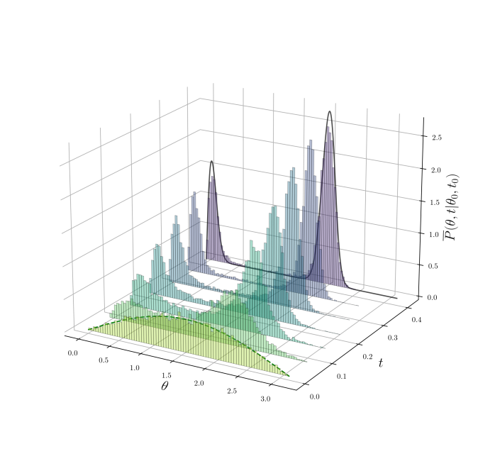
Similarly, the time evolution of the histogram of (shaded-color bars) under the effects of the potential (10b) is shown in figure 6. In this case, the external potential ‘pushes’ the particles towards both poles until they reach a bimodal stationary distribution. Again, a good agreement between our numerical results (shaded-color bars) and the exact stationary distribution, given by equation (17b) and marked in the figure with solid-black line, is noticeable.
The third potential considered in our analysis (10c), namely, , has two minima: one corresponding to stable state (global minimum) and the other to a metastable one (local minimum) as was explained. The initial distribution is marked by the dashed-green-line as before, in this case, it is observed that as time passes a large fraction of the particles gets trapped in the metastable state, as is shown in figure 7 by the particle accumulation around , while the remaining particles do distribute according the equilibrium distribution given by equation (2). Since the time required by the particles to escape from such state is exponentially large in the barrier height, as is established by Kramer’s escape theory, the sampled distribution in our finite-time simulations differs from the corresponding equilibrium distribution solution.
The profile of the ‘metastable distribution’ marked by the solid-black line in figure 7 is obtained as follows: In a finite window of simulation time, the particles that initially were at angles larger than the angle that defines the barrier maximum, , will remain in that region accumulating around the metastable state. Similarly, the particles that initially were at angles smaller than , will remain in that region gathering around the potential global minimum. Therefore, we introduce a ‘returning point’ of an impenetrable potential that splits the interval into two unreachable regions, each one with an appropriate stationary distribution of the form (16). The required profile is computed in such way that the fraction between the number of particles in each region stands in the same relation to the one between the areas of latitudes and , respectively. The equilibrium distribution (16) is recovered from those initial distributions for which their time evolution is not hindered by the energy barrier.


We further analyze the effects of the external potentials on the diffusion of Brownian particles on the sphere, by computing the mean position , the distribution variance (both shown in the top panel of figure 8) and the position autocorrelation function (11) (shown in the lower panel of the same figure). The numerical calculations for the latter case were carried out for an ensemble of Brownian particles.
The relaxation rate towards the stationary distribution strongly depends on the ratio and on the initial distribution if the external potential has metastable states. For , the stationary distribution is close to and a fast relaxation is expected. In contrast, is determined by the minima of if and the relaxation towards the stationary distribution depends on the initial distribution. Indeed, the transition rate towards the stationary distribution is exponentially small if the particles has to overcome an energy barrier to reach the minimum of the potential.
III.3 Stability of Stationary states
Samples of sizes , and , for in the stationary regime were generated from our numerical algorithm with integration step sizes , , , in the cases of free diffusion and under the influence of the potential (10b). Data were gathered from simulations of an ensemble of trajectories at times , with ; is a large enough chosen time that it guarantees that sampling occurs in the stationary regime ( in the cases considered), and is the characteristic time scale. From these data, mean values of the quantity are computed as
| (18) |
where denotes the value of theta in the -th trajectory at time .
The absolute error of with respect the equilibrium value,
| (19) |
computed from the exact stationary distribution given in (16), is given by
| (20) |
| Sample | |||||
|---|---|---|---|---|---|
| 0.001696 | 0.004167 | 0.007578 | 0.011861 | ||
| 0.000433 | 0.000052 | 0.003786 | 0.019382 | ||
| 0.000395 | 0.001056 | 0.001656 | 0.000316 | ||
| 0.000014 | 0.000042 | 0.000233 | |||
| 0.000582 | 0.001775 | 0.004418 | 0.010786 | ||
| 0.001468 | 0.002569 | 0.004387 | 0.009928 | ||
| 0.000020 | 0.000398 | 0.001976 | 0.007509 | ||
| 0.000016 | 0.000025 | 0.000016 | 0.000066 | ||
| 0.001791 | 0.005827 | 0.016737 | 0.046506 | ||
| 0.001136 | 0.005466 | 0.017779 | 0.052353 | ||
| 0.000176 | 0.002395 | 0.012649 | 0.047425 | ||
| 0.000020 | 0.000042 | 0.000061 |
| Sample | |||||
|---|---|---|---|---|---|
| 0.001184 | 0.003358 | 0.008285 | 0.019857 | ||
| 0.000466 | 0.001950 | 0.0019499 | 0.065316 | ||
| 0.000001 | 0.000382 | 0.001815 | 0.006381 | ||
| 0.000041 | 0.000335 | 0.001822 | 0.006857 | ||
| 0.000777 | 0.006259 | 0.024629 | 0.080600 | ||
| 0.000166 | 0.003845 | 0.018739 | 0.065316 | ||
| 0.004103 | 0.004103 | 0.019810 | 0.069621 | ||
| 0.004282 | 0.004282 | 0.020471 | 0.071849 | ||
| 0.002058 | 0.034305 | 0.175293 | 0.628564 | ||
| 0.000220 | 0.040534 | 0.192456 | 0.672770 | ||
| 0.000005 | 0.041133 | 0.193835 | 0.675919 | ||
| 0.000052 | 0.041344 | 0.194492 | 0.677735 |
The absolute error for the firsts four moments of , namely , , and is presented in table 1 for the case of free diffusion, and in table 2 of diffusion under the influence of the external potential (10b).
As expected, for smaller integration step sizes, the error is rather sensible to sample sizes as is observed in the firsts four moments considered for . It can also be noticed that for a chosen integration step size, the error diminishes as the sample size gets large. This trend, however, seems to stops at sample sizes between , thus sample size does not play an important role in error for large enough samples. This effect is observed even earlier for high moments, for instance, no improvement of the error is found in the fourth moment by enlarging the sample size when . From these results, we conclude that this analysis gives a measure the intrinsic error of our numerical algorithm.
Finally, the tolerated error that we may allow ourselves from a given numerical method depends on the particular problem under consideration. Indeed, more exact results might be generated at the expense of more demanding computational power. The analysis presented here might serve to have a starting point to see whether the numerical algorithm may be feasible for a particular problem with a specific associated tolerance.
IV Summary and concluding remarks
In this paper, we presented a numerical algorithm to generate the trajectories of Brownian particles diffusing on the surface of the two-dimensional sphere. The algorithm implemented is based on three-dimensional geometry, thus avoiding the complications introduced by the interpretation of the multiplicative Gaussian-white noise involved in the corresponding stochastic differential equation, and takes into account the effects of an external potential. Our numerical method is weakley convergent, that is, it statistically converges to the solution of the Smoluchowski equation (2).
The algorithm was validated in two scenarios: First, in the absence of external potential, by computing the time dependence histogram of the polar angle, as well as the first two moments, and the time correlation function of the particle positions, from an ensemble of trajectories generated by our algorithm. We observed an excellent agreement at all times between our results and the corresponding quantities obtained from the solution to the diffusion equation on the sphere (7). Second, in the presence of a external potential, for which we calculated the stationary probability distribution when the external potential depends only on . Again, excellent agreement was found between our numerical results and those given by the stationary solutions of the Smoluchoswki equation (2) for three different potentials. In addition, we have also calculated the time correlation of the particle positions for each of these three potentials. Although no analytical solution are available to our knowledge, the traits of correctness are observed. Although we have considered simple potentials, our algorithm can be applied to an arbitrary but physically motivated potential.
An alternative to our numerical algorithm might consider either the numerical integration of the differential stochastic equations that determine the time evolution of or the numerical solution of the Smoluchowski equation (2). However, in any case, this procedure requires to deal with singular terms that diverge at the poles. Although this can be solved by changing from one set of coordinates (chart) to another one, this is however, computationally time consuming.
Acknowledgements.
We acknowledge to the anonymous referees for their thorough and carefully review of the original manuscript. This work was supported by UNAM-PAPIIT IN110120. A.V.G kindly acknowledges the scholarship received from CONACyT and UNAM-PAPIIT IN110120.Appendix A Transformation of the Fokker-Planck equation
The Fokker-Planck equation in Cartesian coordinates is
| (21) |
If we make a coordinate transformation the chain rule implies that this equation transforms accordingly
| (22) |
However, the conditional probability density transforms as where is the determinant of the Jacobian matrix. We would like to rewrite this equation in terms of . For this purpose we need some elementary results from linear algebra. We know that the Jacobian matrix and its inverse , satisfy
| (23) |
so if is the cofactor associated with the term , then this is given by
| (24) |
where is the Jacobian determinant of the inverse matrix . Using this relation we can express the determinant derivative with respect the elements , in the following manner
| (25) |
Now we observe that the partial derivatives of the Jacobian determinant can be related to the components of the Jacobian matrix
Then we can express the derivatives with respect the old coordinates , as functions of the new coordinates in the following manner
| (26) |
Furthermore, it always holds
| (27) |
using the relation 26 we obtain a central result
| (28) |
Compounded twice
But at the same time
Therefore
| (29) |
Using 28 and 29 in the Fokker-Planck equation 21
| (30) |
What allow us to write, if we gather the first derivatives in the same term, the Fokker-Planck in the new coordinates as
| (31) |
This implies the following transformation law for the elements of the Fokker-Planck, in terms of the elements described in the old coordinates .
| (32) | ||||
| (33) | ||||
| (34) |
Just the diffusion matrix , transforms as a (second rank) tensor; the drift vector and the conditional probability density , do not transform as tensors.
Appendix B Stationary sates on
In this section we deduce the stationary solutions of the Fokker-Planck equation. The procedure is discussed in Graham and Haken (1971a) or in Stratonovich (2014). The existence of the stationary solution solution can guaranteed when the conditions of detailed balance are met. In those cases we can get an explicit solution
| (35) |
in which . The drift in B, as is explained in Graham and Haken (1971a) is defined as , which is the reversible part of the drift Graham and Haken (1971b), but in the cases with which we dealt with, it coincides with itself because it is invariant with respect to time inversion (velocities and magnetic fields are not). If we take
| (36) |
being a normalization constant, and plays the role of a generalized thermodynamic potential; these functions are defined even far from thermal equilibrium like in a laser. If we substitute Eq. (36) in Eq. (B), we obtain
If the matrix has an inverse, that we denote by , then we can solve for
| (37) |
Moreover, we may solve for , and reduce the problem to quadratures, if the potential conditions Stratonovich (2014) are satisfied
| (38) |
That is, we might be able to obtain as a line integral over the configuration space variables . So the particular solution for the cases treated in this work is 36, where is given by
| (39) |
where stands for effective potential.
References
- Fujiwara et al. (2002) T. Fujiwara, K. Ritchie, H. Murakoshi, K. Jacobson, and A. Kusumi, The Journal of Cell Biology 157, 1071 (2002).
- Metzler et al. (2016) R. Metzler, J.-H. Jeon, and A. Cherstvy, Biochimica et Biophysica Acta 1858, 2451 (2016).
- Haastert and Devrotes (2004) P. J. M. V. Haastert and P. N. Devrotes, Nature 5, 626 (2004).
- Ma et al. (2004) L. Ma, C. Janetopoulos, L. Yang, P. N. Devrotes, and P. A. Iglesias, Biophysical Journal 87, 3764 (2004).
- van Meer et al. (2008) G. van Meer, D. R. Voelker, and G. W. Feigenson, Nature 9, 112 (2008).
- Meyers et al. (2006) J. Meyers, J. Craig, and D. J. Odde, Current Biology 16, 1685 (2006).
- Hancock (2010) J. T. Hancock, Cell Signalling (Oxford University Press, 2010).
- Furry (1957) W. H. Furry, Phys. Rev. 107, 7 (1957), URL https://link.aps.org/doi/10.1103/PhysRev.107.7.
- Favro (1960) L. D. Favro, Phys. Rev. 119, 53 (1960), URL https://link.aps.org/doi/10.1103/PhysRev.119.53.
- Ivanov (1964) E. Ivanov, Sov. Phys. JETP 18, 1041 (1964).
- Hubbard (1972) P. S. Hubbard, Phys. Rev. A 6, 2421 (1972), URL https://link.aps.org/doi/10.1103/PhysRevA.6.2421.
- Valiev and Ivanov (1973) K. A. Valiev and E. N. Ivanov, Soviet Physics Uspekhi 16, 1 (1973), URL https://doi.org/10.1070/pu1973v016n01abeh005145.
- McClung (1980) R. E. D. McClung, The Journal of Chemical Physics 73, 2435 (1980), eprint https://doi.org/10.1063/1.440394, URL https://doi.org/10.1063/1.440394.
- Graham (1977) R. Graham, Zeitschrift für Physik B Condensed Matter 26, 397 (1977), ISSN 1431-584X, URL https://doi.org/10.1007/BF01570750.
- van Kampen (1986) N. G. van Kampen, Journal of Statistical Physics 44, 1 (1986), ISSN 1572-9613, URL http://dx.doi.org/10.1007/BF01010902.
- Risken (1989) H. Risken, The Fokker-Planck equation Methods of solution and applications, Springer Series in Synergetics (Springer-Verlag, 1989).
- Faraudo (2002) J. Faraudo, The Journal of Chemical Physics 116, 5831 (2002), eprint https://doi.org/10.1063/1.1456024, URL https://doi.org/10.1063/1.1456024.
- Janetopoulos et al. (2004) C. Janetopoulos, L. Ma, P. N. Devrotes, and P. A. Iglesias, Proceedings of the National Academy of Sciences of the United States of America 101, 8951 (2004).
- Castro-Villarreal and Sevilla (2018) P. Castro-Villarreal and F. J. Sevilla, Physical Review E 97, 1 (2018).
- Garduño et al. (2019) F. Sánchez-Garduño, A. L. Krause, J. A. Castillo, and P. Padilla, Journal of Theoretical Biology 481, 136 (2019).
- Castro-Villarreal et al. (2014) P. Castro-Villarreal, A. Villada-Balbuena, J. M. Méndez-Alcaraz, R. Castañeda-Priegoa, and S. Estrada-Jiménez, The Journal of Chemical Physics 140, 1 (2014).
- Yang and Li (2019) Y. Yang and B. Li, The Journal of Chemical Physics 151, 164901 (2019), eprint https://doi.org/10.1063/1.5126201, URL https://doi.org/10.1063/1.5126201.
- Novikov et al. (2020) A. Novikov, D. Kuzmin, and O. Ahmadi, Applied Mathematics and Computation 364, 124670 (2020), ISSN 0096-3003, URL http://www.sciencedirect.com/science/article/pii/S0096300319306629.
- Schnitzer (1993) M. J. Schnitzer, Phys. Rev. E 48, 2553 (1993), URL http://link.aps.org/doi/10.1103/PhysRevE.48.2553.
- Ford et al. (1979) G. W. Ford, J. T. Lewis, and J. McConnell, Phys. Rev. A 19, 907 (1979), URL https://link.aps.org/doi/10.1103/PhysRevA.19.907.
- Ryter and Deker (1980) D. Ryter and U. Deker, Journal of Mathematical Physics 21, 2662 (1980), eprint https://doi.org/10.1063/1.524381, URL https://doi.org/10.1063/1.524381.
- Carlsson et al. (2010) T. Carlsson, T. Ekholm, and C. Elvingson, Journal of Physics A: Mathematical and Theoretical 43, 505001 (2010), URL https://doi.org/10.1088/1751-8113/43/50/505001.
- Gómez (2019) A. Valdés-Gómez, Ph.D Thesis repository (2019), URL https://github.com/AdrianoValdesGomez/PhD-Thesis.
- SupMat (2021) A. Valdés-Gómez and F. J. Sevilla, Supplementary Material (2021).
- Higham (2001) D. J. Higham, SIAM 43, 525 (2001).
- Gardiner (1997) C. W. Gardiner, Handbook of Stochastic Methods for Physics, Chemistry and the Natural Sciences, Springer Series in Synergetics (Springer, 1997), 2nd ed.
- Roberts and Ursell (1960) P. H. Roberts and H. D. Ursell, Philosophical Transactions of the Royal Society of London. Series A, Mathematical and Physical Sciences. 252, 317 (1960).
- Hobson (1965) E. W. Hobson, The theory of Spherical and Ellipsoidal Harmonics (Chelsea Publishing Company New York, 1965).
- Asmar (2005) N. H. Asmar, Partial Differential Equations with Fourier Series and Boundary value problems (Prentice Hall, 2005).
- Jackson (1999) J. D. Jackson, Classical Electrodynamics (John Wiley and Sons Inc, 1999), 3rd ed.
- Ghosh et al. (2012) A. Ghosh, J. Samuel, and S. Sinha, A Letters Journal Exploring The Frontiers of Physics 98 (2012).
- Castro-Villarreal (2014) P. Castro-Villarreal, Journal of Statistical Mechanics: Theory and Experiment 05, 1 (2014).
- Castañeda-Priego et al. (2013) R. Castañeda-Priego, P. Castro-Villarreal, S. Estrada-Jiménez, and J. M. Méndez-Alcaraz (2013), arXiv:1211.5799v2.
- Kubo et al. (1998) R. Kubo, M. Toda, and N. Hashitsume, Statistical Physics II Nonequilibrium Statistical Mechanics, vol. II of Springer Series in Solid-State Sciences (Springer, 1998).
- Graham and Haken (1971a) R. Graham and H. Haken, Z. Physik 243, 289 (1971a).
- Stratonovich (2014) R. L. Stratonovich, Topics in the Theory of Random Noise, vol. I (Martino Publishing, 2014).
- Graham and Haken (1971b) R. Graham and H. Haken, Z. Physik 245, 141 (1971b).