A geometric interpretation for the Delta Conjecture
Abstract.
We introduce a variety , which we call the affine -Springer fiber, generalizing the affine Springer fiber studied by Hikita, whose Borel-Moore homology has an action and a bigrading that corresponds to the Delta Conjecture symmetric function under the Frobenius character map. We similarly provide a geometric interpretation for the Rational Shuffle Theorem in the integer slope case . The variety has a map to the affine Grassmannian whose fibers are the -Springer fibers introduced by Levinson, Woo, and the third author. Part of our proof of our geometric realization relies on our previous work on a Schur skewing operator formula relating the Rational Shuffle Theorem to the Delta Conjecture.
1. Introduction
In this paper, we give geometric realizations of both the Rectangular Shuffle Theorem in the case and for the Delta Conjecture, in terms of affine Springer fibers. This is the second of a two-part series of papers starting with [GGG1], which both algebraically and combinatorially establishes a skewing formula relating the polynomials from the Rectangular Shuffle Theorem and those of the Delta Conjecture, building from the work of [BHMPS]. This skewing formula is key to the proof of our geometric construction.
We summarize the results of the paper in the following table:
| Degree | Algebra | Combinatorics | Geometry | Module |
|---|---|---|---|---|
We explain various objects in the table and relations between them in the following sections. In particular, the first row corresponds to algebraic, combinatorial and geometric avatars of a certain degree symmetric function, while the second row corresponds to a degree symmetric function. The two symmetric functions are related by an explicit skewing operator , see Theorem 1.5.
1.1. Shuffle Theorems
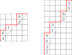
A labeled Dyck path or parking function is a Dyck path in the grid whose vertical steps are labeled with positive integers, such that the labeling increases up each vertical run. See the left-most example in Figure 1. The Shuffle Theorem [CM] gives the following remarkable combinatorial formula for the evaluation ,
| (1) |
See Section 2 for relevant definitions. Similarly, given one can define a rational parking function as a lattice path (also known as a rational Dyck path) in the grid that stays weakly above the line , starts in the southwest corner, and ends in the northeast corner, together with a column-strictly-increasing labeling of the up steps (see the middle path in Figure 1 for an example where , and ). The combinatorial statistics and in the “combinatorial” right hand side of (1) has a natural generalization to rational parking functions.
However, to generalize the “algebraic” left hand side one needs to consider the Elliptic Hall Algebra defined in [EHA] and extensively studied in the last two decades [RationalShuffle, BHMPS, BHMPS2, GN, SV1, SV2, Negut]. This is a remarkable algebra acting on the space of symmetric functions in infinitely many variables with coefficients in . The Rational Shuffle Theorem, proposed by Bergeron, Garsia, Leven and Xin [RationalShuffle] (see also [GN] for case and a connection to Hilbert schemes), subsequently proven by Mellit [Mellit], states that
where is a particular element of . Note that our conventions for and are flipped from [RationalShuffle].
We will be primarily interested in the case where (so that and ) and consider parking functions in the rectangle. The corresponding symmetric function has degree .
Remark 1.1.
For we have , and the symmetric function in question is .
1.2. Affine Springer fibers
In a different line of work, Hikita [Hikita] gave an alternative geometric interpretation for in terms of affine Springer fibers. Given a nil-elliptic operator , one can define the affine Springer fiber in the affine flag variety . The group has a Springer-like representation in the (Borel-Moore) homology of . Affine Springer fibers and their homology have been a subject of very active study in geometric representation theory, see [Yun] and references therein. In particular, is closely related to compactified Jacobians and Hilbert schemes of points on plane curve singularities [MY, MS, MaulikShen] and serves as a local model for fibers in the Hitchin integrable system [OY, OY2], while the point count of over a finite field is related to orbital integrals in number theory [KivTsai]. The conjectures of Oblomkov, Rasmussen and Shende [ORS] relate the homology of affine Springer fibers to Khovanov-Rozansky link homology.
If is regular and semisimple, the geometry of is controlled by the characteristic polynomial and the spectral curve . Hikita considered in [Hikita] the case when
and proved that admits an affine paving with cells in bijection with parking functions and the (Frobenius) character of the Borel-Moore homology of (as a bigraded -module) matches the right hand side of (1) (up to a minor twist). In particular, the dimension of the cells is closely related to the statistics on parking functions. In [CO] Carlsson and Oblomkov used this work to construct a long-sought explicit basis in the space of diagonal coinvariants.
In [GMV] the second author, Mazin and Vazirani generalized the results of [Hikita] to -parking functions with (and in the above notations): for
the affine Springer fiber also admits an affine paving with cells in bijection with parking functions. In particular, [GMV] clarified the relation between parking functions and a certain subset of (extended) affine permutations in .
In [GMO] the second author, Mazin and Oblomkov made progress towards the general non-coprime case by considering a more complicated class of “generic” spectral curves . They proved that for such the affine Springer fiber in the affine Grassmannian admits an affine paving with cells labeled by -Dyck paths. It is plausible that the affine Springer fiber also admits an affine paving with cells labeled by parking functions, but we do not need it here.
Instead, we propose a different geometric model for a special subclass of the non-coprime case. Let , we consider a family of nil-elliptic elements with characteristic polynomials .
Definition 1.2.
Let be the -linear operator on defined by
Here we extend the basis periodically by . We also define a certain union of affine Schubert cells and the subvariety
We can now state our first main result:
Theorem 1.3.
-
(a)
For the space does not depend on and admits an affine paving in which the cells are in bijection with parking functions.
-
(b)
For all , the Borel-Moore homology of has an action of . For the Frobenius character of this action equals
where the parameter keeps track of homological degree and the grading keeps track of the connected component of .
It would be interesting to find the analogues of for more the more general family of symmetric functions where and are coprime.
Remark 1.4.
For we have for , and . For , we recover Hikita’s result but with a slightly different variety. In particular, is a non-compact subvariety of the affine partial flag variety associated to , and the space has one connected component for each possible value of the area statistic on an Dyck path. On the other hand, Hikita studied the affine Springer fiber associated to the operator inside of , which is a compact subvariety of the affine flag variety associated to . The content of Theorem 1.3 in the case then says that the affine Springer fiber studied by Hikita has the same Borel–Moore homology as that of , even though the spaces are not isomorphic.
1.3. Delta Conjecture
A second generalization of the Shuffle Theorem called the Delta Conjecture was formulated by Haglund, Remmel, and Wilson [HRW]. It involves a more general Macdonald eigenoperator and relates it to stacked parking functions. See the image on the right of Figure 4 for an example of a stacked parking function for and . The (Rise) Delta Conjecture (reformulated here in terms of stacked parking functions) states
This version of the Delta Conjecture was proven by [DAdderio] and independently by [BHMPS]. To the authors’ knowledge, the Valley version (involving a statistic ) of the conjecture remains open.
In [GGG1], we proved a formula that directly relates the Rational Shuffle Theorem to the Delta Conjecture.
Theorem 1.5 ([GGG1, Theorem 1.1]).
Letting and , we have
| (2) |
where is the adjoint to multiplication by the Schur function .
The proof uses the relation between the Elliptic Hall Algebra and the Shuffle algebra and certain identities for studied in [BHMPS, BHMPS2, Negut].
Our main result is a geometric version of (2) by constructing a family of subvarieties in the partial affine flag variety:
where above is dominance order on partitions. Equivalently, the Jordan type condition above may be written . See Definition LABEL:def:Varieties for more details, here we identify the affine partial flag variety with the space of flags of lattices, and refers to the Jordan type of the induced action of on the quotient .
Theorem 1.6.
-
(a)
For all , the space does not depend on , and its Borel-Moore homology admits an action of such that
where .
-
(b)
We have
where the parameter keeps track of homological degree and the grading keeps track of the connected component of .
In fact, part (b) follows from Theorem 1.5 and part (a). Part (a) is proved similarly to the main result of [GG], see below.
Remark 1.7.
In the case , Theorem 1.6 part (a) is trivial. Indeed, when we get since and the Jordan type condition is vacuous. On the other hand, and
Lastly, we use Theorem 1.5 and the Rational Shuffle Theorem to give a new combinatorial proof of the (Rise) Delta Conjecture.
1.4. -Springer fibers
In a previous work, the first and third authors [GG] studied a family of varieties called -Springer fibers (see also [Griffin, Griffin2, GLW]). We use an equivalent definition following [GG, Lemma 3.3].
Definition 1.8.
Fix a partition with and an integer , and define . Also, fix a nilpotent operator on with Jordan type . Then the -Springer fiber is defined as the space of partial flags
such that and . Note that here we have indexed the parts of the flag in order to match our convention for indexing flags of lattices. Further note that the Jordan type condition may be replaced with .
One of the main results of [GG] gives a representation-theoretic description for the cohomology of -Springer fiber.
Theorem 1.9 ([GG]).
There is an action of in the cohomology of . The corresponding graded Frobenius character equals
where is the modified Hall-Littlewood polynomial.
We can relate the variety to the -Springer fibers as follows: consider the projection to the affine Grassmannian
which sends a flag of lattices to .
Theorem 1.10.
Each fiber of the projection is either empty or isomorphic to a -Springer fiber for some .
To prove Theorem 1.10, we consider the -dimensional space , and the partial flag . The operator is given by the restriction of to , and the key Lemma LABEL:lem:eval-in-sub shows that it has Jordan type for some . Now the conditions defining translate to the conditions for , see Section LABEL:sec:_geometry for details.
The proof of Theorem 1.9 heavily used the work of Borho and MacPherson [BM] on partial resolutions of the nilpotent cone. Note that by [HottaSpringer] the modified Hall-Littlewood polynomial in the Theorem 1.9 can be interpreted as the graded Frobenius character of the homology of the classical Springer fiber, which coincides with the fiber of the projection .
We use this idea to develop a sheaf-theoretic generalization of Theorem 1.9, and use it to prove Theorem 1.5(a).
Remark 1.11.
Note that the discussion above and Theorem 1.10 do not imply that and expand positively in terms of Hall-Littlewood symmetric functions, even in the case of . This is because the projection maps from and to are not fiber bundles over the cells in the Schubert cell decomposition of . We invite the reader to check that the fibers of over depend on : Generically, is isomorphic to the Springer fiber associated to a nilpotent matrix of Jordan type , but over the torus fixed point of the Schubert cell is isomorphic to the Springer fiber for Jordan type .
1.5. Organization of the paper
The paper is organized as follows. In Section 2, we give a combinatorial background on symmetric functions, parking functions and affine permutations. In Section 3, we translate parking function combinatorics and diagonal inversions in terms of a class of affine permutations called -restricted, and we prove several useful lemmas concerning them. Sections LABEL:sec:_geometry, LABEL:sec:_Springer_action, and LABEL:sec:_X_dimensions are focused on the geometry of affine Springer fibers. In Section LABEL:sec:_geometry we introduce the varieties and and prove Theorem 1.6(a). In Section LABEL:sec:_Springer_action, we use Springer theory and work of Borho and MacPherson to show there are compatible symmetric group actions on the Borel-Moore homologies of and . We then prove Theorem 1.6(a), a geometric version of the skewing formula. In Section LABEL:sec:_X_dimensions, we construct an affine paving of . This allows us to prove Theorem 1.3 and complete the proof of Theorem 1.6(b).
1.6. Future directions
We conclude the introduction with a few possible further directions.
In particular, our varieties depend on a parameter . However, we show in Theorems 1.3 and 1.6 that when these varieties are independent of and the graded Frobenius character of their Borel-Moore homologies give the symmetric functions in the Rational Shuffle Theorem and Delta Theorem. However, when , there exist examples of (respectively ) whose Borel-Moore homology groups differ from the terms in the Rational Shuffle Theorem (respectively Delta Theorem). Therefore, one could define new symmetric functions and by
Problem 1.12.
Find combinatorial and Macdonald operator formulas for and in the cases that generalize those on either side of the Rational Shuffle and Delta Theorems.
Another natural question is whether our varieties can be generalized to give geometric interpretations of other symmetric functions coming from Macdonald-theoretic or Elliptic Hall Algebra operators.
Acknowledgments
We thank François Bergeron, Eric Carlsson, Mark Haiman, Jim Haglund, Oscar Kivinen, Jake Levinson, Misha Mazin, Anton Mellit, Andrei Negu\cbt, Anna Pun, George Seelinger, and Andy Wilson for useful discussions.
2. Notation and Background
2.1. Symmetric functions
We refer to [Macdonald] for details on many of the standard definitions in this section. We will work in the ring of symmetric functions in infinitely many variables over . We will use elementary symmetric functions
where is a partition. We also have monomial symmetric functions
where is any tuple of distinct positive integers such that whenever . Both and form a basis of .
We also use the basis of Schur functions , defined as where the coefficients are the Kostka numbers, which count the number of column-strict Young tableaux of shape and content . We draw our Young tableaux in French notation:
and the above tableau has content , with the th entry indicating the multiplicity of in the tableau. Its shape is , indicating the length of each row from bottom to top.
Definition 2.1.
The Hall inner product on is defined by
and extending by linearity, using the fact that forms a basis of .
The Schur functions and Hall inner product are directly tied to the representation theory of the symmetric group . The irreducible representations of are indexed by partitions of , and the Frobenius map takes a representation to . Clearly is additive across direct sum, and it has the remarkable property of being multiplicative across induced tensor product:
We make use of a (doubly) graded version of the Frobenius map as follows.
Definition 2.2.
Given a graded module , its graded Frobenius character is
For a doubly-graded module , we write
We use the adjoint operators to multiplication operators with respect to the Hall inner product.
Definition 2.3.
The operator is defined such that the identity
holds for all symmetric functions (resp. ).
We will make use of the following lemma from [GG].
Lemma 2.4.
[GG, Lemma 2.1] Given an -module, a Young subgroup, and a partition , then
where is the -isotypic component of the restriction of to an -module, whose Frobenius character is taken as an -module.
2.2. Rational parking functions
Throughout this subsection, let and be positive integers such that . Let be the set of rational Dyck paths (height and width ), and let be the labeled parking functions on elements of . That is, the set of labelings of the vertical runs of elements of by positive integers such that the labeling weakly increases up each vertical run.
Definition 2.5.
The area of an element of is the number of whole boxes lying between the path and the diagonal, so that the diagonal does not pass through the interior of the box.
Definition 2.6.
The dinv statistic (for “diagonal inversions”) on is defined as
where is the Dyck path of . We define each of these three quantities separately below.
To define , recall that the arm of a box above a Dyck path in the grid is the number of boxes to its right that still lie above the Dyck path. The leg is the number of boxes below it that still lie above the Dyck path.
Definition 2.7.
The pathdinv of Dyck path from to (with ) is the number of boxes above the Dyck path of for which
Remark 2.8.
We call this statistic here to emphasize that it only depends on the rational Dyck path, and to distinguish it from of the parking function. It was simply called in [RationalShuffle].
To define the statistic on rational parking functions, we use the same conditions on pairs of boxes identified in Lemma 2.14, which we call attacking pairs.
Definition 2.9.
A diagonal in the by grid, where , is a set of boxes whose lower left hand corners pairwise differ by a multiple of .
The main diagonal of the by rectangle is the line between and . Note that we use Cartesian coordinates in the first quadrant for the boxes and label each box’s position by the coordinates of its lower left hand corner.
A pair of boxes in a by grid (with ) is an attacking pair if and only if either:
-
•
and are on the same diagonal, with to the left of , or
-
•
is one diagonal below , and to the right of .
Remark 2.10.
When boxes are known to be labeled, we often use the name of the box and its label interchangeably, as in the definition below.
Definition 2.11.
The tdinv of is the number of attacking pairs of labeled boxes in such that .
Definition 2.12.
The maxtdinv of a Dyck path is the largest possible of any parking function of shape .
Note that can be achieved by taking of the labeling of obtained by labeling using across diagonals from left to right, starting from the bottom-most diagonal and moving upwards. Alternatively, is the number of attacking pairs such that and are boxes directly to the right of an up-step of .
Define the rank of the box in row and column of the rectangle to be
In other words, we put in the box in the SW corner, and fill the rest of the ranks by increasing them by or , respectively, as we go North from to if is not divisible or divisible by , respectively. As we go East from to , we decrease by . The ranks of the boxes in the case of and is shown in Figure 2.
The following is easily verified and we omit the proof.
Proposition 2.13.
All ranks above the diagonal are strictly positive, and pairwise distinct. The ranks in different rows have different remainders mod . All ranks below or on the diagonal are nonpositive.
We will need the following statement relating ranks to attacking pairs.
Lemma 2.14.
Suppose are two boxes inside the rectangle. Then if and only if form an attacking pair.
Proof.
First observe that each diagonal has at most one box in each block and that the ranks on the same diagonal increase by from left to right since for each box ,
For the reverse implication, we consider the following cases:
Case 1. Suppose the boxes containing and form an attacking pair on the same diagonal, with to the left of . Then we have because the ranks on a diagonal increase by and there are columns.
Case 2. Suppose the boxes containing and form an attacking pair with to the right of where is in one lower diagonal than . Letting be the entry below , we have for some with since and are on the same diagonal. Then is either equal to or , so .
We now show that if two squares do not form an attacking pair, then one of the inequalities is not satisfied. If is to the right of in its diagonal, or left of in one higher diagonal, the inequality is not satisfied by the cases above. So we can assume the two boxes are at least two diagonals apart. But if the largest entry in the lower diagonal is , then the smallest entry two diagonals up is equal to and so we cannot have the inequality satisfied. ∎
Definition 2.15.
We write for the number of boxes that lie fully above the diagonal in the rectangle, which is equal to .
We now show a correspondence between certain attacking pairs and the complement squares to those that contribute to pathdinv. To do so, we first rephrase the definition of pathdinv in a way that we used in [GGG1]. The proof simply follows from analyzing both sides of the inequality in Definition 2.7, and we omit it.
Lemma 2.16.
The statistic is the number of boxes above such that, if is the slope of the diagonal, we have
Lemma 2.17.
For a Dyck path the difference equals the number of attacking pairs of boxes such that is to the left of a vertical step in , and is between and the main diagonal.
Proof.
We outline the proof of essentially the same fact shown in [GorskyMazin, Lemma 2.22], though we note that their figures are flipped upside down and transposed from ours, and we translate the main steps here in our notation.
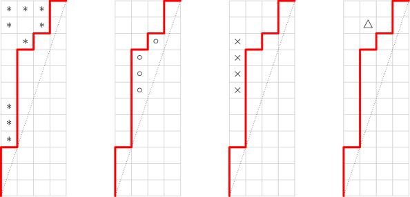
In Figure 3, the boxes contributing to are marked with . We know that is the number of boxes fully above the diagonal that are not marked with , and we sort them into three types:
-
•
Below : We mark these boxes with a .
-
•
Above , “too high”: These squares have , in other words, their leg is too long to be marked with . We mark these with .
-
•
Above , “too low”: These squares have , in other words, their leg is too short. We mark these with .
For each entry, we draw a line to the right until we cross a vertical step of ; let be the box just to the left of this vertical step. Then by the height condition for , there is a box above the diagonal and below in the same column as that is one diagonal above . We match the square to this attacking pair , as shown at left below. Conversely, every such off-diagonal pair corresponds to a triangle.
![[Uncaptioned image]](https://cdn.awesomepapers.org/papers/2ba03b2b-9ae4-402b-8545-95e5dc44cfb6/x3.png)
We now consider a square marked with . We first reflect vertically as follows: let be the number of squares vertically between and the path , and define to be the square in the same column as that has exactly squares vertically below it in the grid (starting at the bottom below the diagonal). Then, let be the square to the left of the vertical step of in the row of , and the square in the column of on the same diagonal as . By an analysis of the heights involved, one sees that is indeed a square between the path and the diagonal, and so form an attacking pair of the desired form. We match with the attacking pair as shown at middle above. By the work in [GorskyMazin], this association is bijective with the attacking pairs formed by taking a square between the diagonal and and matching it with the entry on its diagonal just outside of that is farthest to the left.
The remaining pairs are matched with ’s as shown at right above, via the following algorithm. Given a square marked with , we move exactly columns to the right, and in the new column we find the square below whose vertical distance to equals . Then the row of determines the entry to its left, and the entry is the unique entry in the column of in the same diagonal as . This again is a bijection with the remaining pairs by the work in [GorskyMazin]. ∎
2.3. Stacked parking functions
We use the notation of [GGG1, HRW] here, and recall the definition of a stacked parking function that can be used to reformulate the Rise version of the Delta conjecture.
Definition 2.18.
A stack of boxes in an grid is a subset of the grid boxes such that there is one element of in each row, at least one in each column, and each box in is weakly to the right of the one below it.
A stacked parking function with respect to is a labeled lattice path with north and east steps from to such that each box of lies below the path of , and the labeling is strictly increasing up each column. (See the right hand diagram in Figure 4.)
We write is the set of stacked parking functions with respect to , and
We will also need the following construction from [GGG1] relating rational parking functions with the stacked ones. Set . Given a standard parking function in the rectangle, we call a label big if , and small if . We denote by the number of big labels in the -th column, and by the number of small labels. Note that
| (3) |
Definition 2.19.
A -parking function is called admissible if for all .
We construct a map from the set of standard admissible parking functions to the set as follows:
-
•
The parking function is obtained by erasing all big labels in and the north steps to the left of them.
-
•
In particular, the length of the th vertical run of the lattice path for is equal to .
-
•
The height of the stack in column is given by .
See Figure 4 for an example.
Lemma 2.20.
[GGG1, Lemma 4.7] The stacked parking function is well defined in . We have a bijection between and the quotient of the set of admissible parking functions by the action of which permutes the big labels.
One can define the analogues of and statistics for stacked parking functions. These appear in the Delta Theorem, but we do not need them in this paper and refer to [GGG1, Section 4.1] for all definitions and a detailed discussion.
2.4. Affine permutations
We now establish notation on affine permutations.
Definition 2.21.
An (extended) affine permutation in is a bijection such that, for all ,
We will often write the affine permutations in window notation
In order for to be well defined, we need to have pairwise distinct remainders modulo . By reducing modulo , we get a projection .
Definition 2.22.
The degree of an affine permutation is
| (4) |
One can check that is always an integer and
Definition 2.23.
Given , we define the translation by
We have Furthermore, any affine permutation can be uniquely written as
| (5) |
Definition 2.24.
We say that an affine permutation is positive if for . Equivalently, and for . We denote the set of positive affine permutations by .
Definition 2.25.
We say that an affine permutation is normalized, if , that is, the values in the window contain . Equivalently, we require that . We denote by the set of normalized affine permutations, and by the set of positive and normalized affine permutations.
Remark 2.26.
We have a right action of on . Note that for we have
In particular, the right action of preserves the sets and .
3. Combinatorics of -restricted permutations
In this section, we establish some combinatorial results on a special affine permutation that will correspond to the nil-elliptic element used to construct the affine Springer fibers in the sections below. The facts proven here will help with dimension counting.
3.1. Definition and setup
We will need a special affine permutation defined as follows:
| (6) |
Remark 3.1.
Observe that for a box in row and column in the rectangle such that , the rank of the box immediately above satisfies
Furthermore, the boxes with which are above the main diagonal are exactly those for which is not divisible by , so that either (if is divisible by ) or (if is not divisible by ).
Lemma 3.2.
The affine permutation is well defined in . Its projection to is a single -cycle.
Proof.
It is sufficient to prove the second claim. By iterating and reducing modulo , we get
This completes the proof. ∎
Example 3.3.
For , , , we have
Its projection to is in list notation, which in cycle notation is
Definition 3.4.
We say that an affine permutation is -restricted if:
-
•
is positive and normalized, and
-
•
for all .
Example 3.5.
The affine permutation
is -restricted for as in Example 3.3, because is to the right of , is to the right of (which appears to the left of the window), is to the right of (which appear consecutively just to the left of the window), and so on.
Example 3.6.
We will often consider the inverse of a -restricted affine permutation; for the example above, we have
Definition 3.7.
An inversion of an affine permutation is a pair of entries such that lies in the window (that is, ), , and occurs to the left of (that is, ). Note that may be to the left of the window.
We write to denote the number of inversions of .
Example 3.8.
The inversions in the affine permutation above are
Thus . Note that for any affine permutation , and so above we would find as well.
3.2. Relating rational parking functions and affine permutations
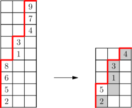
Let be a parking function with Dyck path . We consider the following additional labeling: to the right of each vertical step of we write the parking function label as usual, and to the left we write the rank of the corresponding box, as in Figure 5.
Definition 3.9.
To a parking function we associate an affine permutation such that is the rank of the box in the same row as, and just to the left of, the parking function label .
Example 3.10.
The parking function in Figure 5 corresponds to the affine permutation
which is -restricted as shown above. Note that where
and .
Lemma 3.11.
The map is a bijection between the set of parking functions and the set of -restricted affine permutations, for any fixed .
Proof.
We first show that is always -restricted. By Proposition 2.13 the values are all positive and have pairwise distinct remainders modulo , so is a well-defined positive affine permutation. Furthermore, the vertical step at the southwest corner has rank 1, so is normalized.
Next, consider two vertical steps in consecutive rows of with parking function labels and , and let be the horizontal distance between them (see Figure 6). Let . Then is the rank of the box just above by Remark 3.1 since the parking function label is not in the top row of the rectangle (see Remark 3.1).
We have , so that . If , then by the parking function condition. If , then , so again we have . Finally, for in the top row we have . Since , we get
We have shown the image of under the map is a -restricted affine permutation; we now construct the inverse map. Given a -restricted affine permutation , we construct the rational Dyck path by placing vertical steps to the right of the ranks corresponding to the values for . Since is positive, by Proposition 2.13 all the vertical steps are to the left of the diagonal. Since is normalized, there is a vertical step at the southwest corner of the rectangle. Since is an affine permutation, there is one vertical step in each row.
We now show that the vertical steps move weakly to the right from bottom to top, forming a Dyck path by connecting the runs of vertical steps horizontally. For a pair of consecutive vertical steps labeled as in Figure 6 (where may be negative) the inequality is equivalent to . Thus , so we do indeed have a well-defined Dyck path.
We then label the box to the right of the vertical step labeled by for each . To check that this gives a parking function, either and (and satisfies the parking function condition) or is to the right of . The reverse map clearly inverts the forward map, so the proof is complete. ∎
The following lemma is clear from Lemma 3.11, which is a fact we will need in later sections.
Lemma 3.12.
If is -restricted, then for all .
We now use Lemma 2.17 to translate the statistic into the language of affine permutations as follows.
Lemma 3.13.
For any and , we have
Proof.
Let be the Dyck path of . Since , we have
By Lemma 2.17, the quantity counts the number of attacking pairs of boxes such that is to the left of a vertical step in and is between and the main diagonal. We claim these pairs correspond to the pairs satisfying the stated conditions and also having .
Indeed, let be the rank of box and the rank of box ; then is the parking function label of to the right of . Since is below , we have that is a rank of a vertical step for some , so we have that is a parking function label between and inclusive. But then that means . In fact, this analysis shows if and only if is below . By Lemma 2.14, we have , and since we assumed is abo