A Generalized Neural Diffusion Framework on Graphs
Abstract
Recent studies reveal the connection between GNNs and the diffusion process, which motivates many diffusion-based GNNs to be proposed. However, since these two mechanisms are closely related, one fundamental question naturally arises: Is there a general diffusion framework that can formally unify these GNNs? The answer to this question can not only deepen our understanding of the learning process of GNNs, but also may open a new door to design a broad new class of GNNs. In this paper, we propose a general diffusion equation framework with the fidelity term, which formally establishes the relationship between the diffusion process with more GNNs. Meanwhile, with this framework, we identify one characteristic of graph diffusion networks, i.e., the current neural diffusion process only corresponds to the first-order diffusion equation. However, by an experimental investigation, we show that the labels of high-order neighbors actually exhibit monophily property, which induces the similarity based on labels among high-order neighbors without requiring the similarity among first-order neighbors. This discovery motives to design a new high-order neighbor-aware diffusion equation, and derive a new type of graph diffusion network (HiD-Net) based on the framework. With the high-order diffusion equation, HiD-Net is more robust against attacks and works on both homophily and heterophily graphs. We not only theoretically analyze the relation between HiD-Net with high-order random walk, but also provide a theoretical convergence guarantee. Extensive experimental results well demonstrate the effectiveness of HiD-Net over state-of-the-art graph diffusion networks.
Introduction
Graphs, such as traffic networks, social networks, citation networks, and molecular networks, are ubiquitous in the real world. Recently, Graph Neural Networks (GNNs), which are able to effectively learn the node representations based on the message-passing manner, have shown great popularity in tackling graph analytics problems. So far, GNNs have significantly promoted the development of graph analysis towards real-world applications. e.g, node classifification (Abu-El-Haija et al. 2019; Lei et al. 2022; Wang et al. 2017), link prediction (Kipf and Welling 2016b; You, Ying, and Leskovec 2019), graph reconstruction (Ouyang et al. 2023), subgraph isomorphism counting (Yu et al. 2023), and graph classifification (Gao and Ji 2019; Zhang et al. 2018).
Some recent studies show that GNNs are in fact intimately connected to diffusion equations (Chamberlain et al. 2021; Wang et al. 2021; Thorpe et al. 2022), which can be considered as information diffusion on graphs. Diffusion equation interprets GNNs from a continuous perspective (Chamberlain et al. 2021) and provides new insights to understand existing GNN architectures, which motives some diffusion-based GNNs. For instance, (Wang et al. 2021) proposes continuous graph diffusion. (Thorpe et al. 2022) utilizes the diffusion process to handle oversmoothing issue. (Song et al. 2022) considers a graph as a discretization of a Riemannian manifold and studies the robustness of the information propagation process on graphs. Diffusion equation can also build a bridge between traditional GNNs and control theory (Zang and Wang 2020). Although the diffusion process and graph convolution are closely related, little effort has been made to answer: Is there a unified diffusion equation framework to formally unify the current GNN architectures? A well-informed answer can deepen our understanding of the learning mechanism of GNNs, and may inspire to design a broad new class of GNNs based on diffusion equation.
Actually, (Chamberlain et al. 2021) has explained GCN (Kipf and Welling 2016a) and GAT (Veličković et al. 2017) from diffusion equation. However, with more proposed GNN architectures, it is highly desired to formally revisit the relation between diffusion equation and GNNs. In this paper, we discover that many GNN architectures substantially can be unified with a general diffusion equation with the fidelity term, such as GCN/SGC [22], APPNP[14], GAT [19], AMP [16], DAGNN [15]. Basically, the diffusion equation describes that the change of a node representation depends on the movement of information on graphs from one node to its neighbors, and the fidelity term constraints that the change of a node representation depends on the difference with its initial feature. Furthermore, we show that the unified diffusion framework can also be derived from an energy function, which explains the whole framework as an energy minimization process in a global view. Compared with other unified frameworks (Zhu et al. 2021; Ma et al. 2021), our framework is from the diffusion perspective, which has many advantages. For example, diffusion-based methods are able to address the common plights of graph learning models such as oversmoothing (Chamberlain et al. 2021; Wang et al. 2021). What’s more, the diffusion equation can be seen as partial differential equations (PDEs) (Chamberlain et al. 2021), thus introducing many schemes to solve the graph diffusion equation such as explicit scheme, implicit scheme, and multi-step scheme, some of which are more stable and converge faster.
Based on the above findings, we can see that the diffusion process employed by most current GNNs just considers the first-order diffusion equation, which only diffuses messages among 1-hop neighbors. That is, the first-order diffusion has the underlying homophily assumption among 1-hop neighbors. While we empirically discover that the labels of 2-hop neighborhoods actually appear monophily property (Altenburger and Ugander 2018), i.e., nodes may have extreme preferences for a particular attribute which are unrelated to their own attribute and 1-hop neighbors’ attribute, but are more likely to be similar with the attribute of their 2-hop neighbors. Simply put, monophily can induce a similarity among 2-hop neighbors without requiring similarity among 1-hop neighbors. So when the 1-hop neighbors are heterophily-dominant or have noise, the 2-hop neighbors will provide more relevant context. Therefore, a more practical diffusion process should take both the first-order and second-order neighbors into account. How can we design a new type of graph diffusion networks satisfying the above requirement based on our framework?
In this paper, we design a new high-order neighbor-aware diffusion equation in our proposed diffusion framework, and then derive a High-order Graph Diffusion Network (HiD-Net). Specifically, our model simultaneously combines the first-order and second-order diffusion process, then we regularize the diffusion equation by minimizing the discrepancy between the estimated and the original graph features. The whole diffusion equation is finally integrated into the APPNP architecture. With second-order diffusion equation, HiD-Net is more robust against the attacks and more general on both homophily and heterophily graphs. We theoretically prove that HiD-Net is essentially related with the second-order random walk. We also provide the convergence guarantee that HiD-Net will converge to this random walk’s limit distribution as the number of layers increases, and meanwhile, the learned representations do not converge to the same vector over all nodes. The contributions of this paper are summarized as follows:
-
•
We propose a novel generalized diffusion graph framework, consisting of diffusion equation and fidelity term. This framework, formally establishing the relation between diffusion process with a wide variety of GNNs, describes a broad new class of GNNs based on the discretized diffusion equations on graphs and provides new insight to the current graph diffusion/neural networks.
-
•
We discover the monophily property of labels, and based on our diffusion framework, we propose a high-order graph diffusion network, HiD-Net, which is more general and robust. We theoretically build the relation between HiD-Net and second-order random walk, together with the convergence guarantee.
-
•
Our extensive experiments on both the homophily and heterophily graphs clearly show that HiD-Net outperforms the popular GNNs based on diffusion equation.
Related Work
Graph convolutional networks. Recently, graph convolutional network (GCN) models (Bruna et al. 2013; Defferrard, Bresson, and Vandergheynst 2016; Kipf and Welling 2016a; Veličković et al. 2017; Hamilton, Ying, and Leskovec 2017) have been widely studied. Based on the spectrum of graph Laplacian, (Bruna et al. 2013) generalizes CNNs to graph signal. Then (Defferrard, Bresson, and Vandergheynst 2016) further improves the efficiency by employing the Chebyshev expansion of the graph Laplacian. (Kipf and Welling 2016a) proposes to only aggregate the node features from the one-hop neighbors and simplifies the convolution operation. (Veličković et al. 2017) introduces the attention mechanisms to learn aggregation weights adaptively. (Hamilton, Ying, and Leskovec 2017) uses various ways of pooling for aggregation. More works on GNNs can be found in surveys (Wu et al. 2020b; Zhou et al. 2020).
Diffusion equation on graphs. Graph Heat Equation (GHE) (Chung and Graham 1997), which is a well-known generalization of the diffusion equation on graph data, models graph dynamics with applications in spectral graph theory. GRAND (Chamberlain et al. 2021) studies the discretized diffusion PDE on graphs and applies different numerical schemes for their solution. GRAND++ (Thorpe et al. 2022) mitigates the oversmoothing issue of graph neural networks by adding a source term. DGC (Wang et al. 2021) decouples the terminal time and propagation steps of linear GCNs from a perspective of graph diffusion equation, and analyzes why linear GCNs fail to benefit from deep layers. ADC (Zhao et al. 2021) strategies to automatically learn the optimal diffusion time from the data. However, these works focus on specific graph diffusion network, thus there is not a framework to formally unify the GNNs.
The unified GNN framework. (Zhu et al. 2021) establishes a connection between different propagation mechanisms with a unified optimization problem, and finds out that the proposed propagation mechanisms are the optimal solution for optimizing a feature-fitting function over a wide class of graph kernels with a graph regularization term. (Ma et al. 2021) establishes the connections between the introduced GNN models and a graph signal denoising problem with Laplacian regularization. It essentially is still an optimization solving framework from the perspective of signal denoising. However, our framework is based on the diffusion equation, where the advantages are two fold: one is that diffusion-based methods are able to address the oversmoothing problem (Chamberlain et al. 2021; Wang et al. 2021). The other is that the diffusion equation can be seen as partial differential equations (PDEs) (Chamberlain et al. 2021) and thus can introduce many schemes that have many good properties such as fast convergence rate and high stability.
The Generalized Diffusion Graph Framework
Notations. Consider an undirected graph as with adjacency matrix , where contains nodes and is the set of edges. The initial node feature matrix is denoted as , where is the dimension of node feature. We denote the neighbors of node at exactly hops/steps away as . For example, are the immediate neighbors of .
Diffusion is a physical process that equilibrates concentration differences without creating or destroying mass. This physical observation can be easily cast in the diffusion equation, which is a parabolic partial differential equation. Fick’s law of diffusion describes the equilibration property (Weickert 1998):
| (1) |
where is the diffusion flux, which measures the amount of substance that flows through a unit area during a unit time interval. is the diffusivity coefficient, which can be constant or depend on time and position. is the concentration gradient. This equation states that a concentration gradient causes a flux which aims to compensate for this gradient. The observation that a change in concentration in any part of the system is due to the influx and outflux of substance into and out of that part of the system can be expressed by the continuity equation:
| (2) |
where denotes the time. Plugging in Fick’s law (1) into the continuity equation we end up with the diffusion equation:
| (3) |
As is the sum of the second derivatives in all directions, please note that normal first order derivatives and second order derivatives are on continuous space and can not be generalized directly to graph which is on discrete space. As (Chamberlain et al. 2021) defined, the first derivative is the difference between the feature of a node and its neighbor. And the second derivative can be considered as the difference between the first derivatives of the node itself and its neighbors.
For better illustration, we provide an example. Consider a chain graph in Figure 1, where , , and are the indexes of the nodes. The feature of node is denoted as .

The first order derivatives on node is defined as and . The diffusion flux from node to node at time on a graph is:
| (4) |
The second order derivative is the difference of first order derivatives: . We notice that the chain graph only has one dimension, so the divergence of node on a chain graph is equal to its second order derivative: .
Thus, on a normal graph, we have the generalized form: .
Here we normalize the diffusion process utilizing the degree of the nodes to down-weight the high-degree neighbors, and we have , where is the element of , and .
So the diffusion equation on node can be defined as:
| (5) | ||||
The diffusion equation models the change of representation with respect to , which depends on the difference between the nearby nodes, implying that the greater the difference between a node and its neighbors, the faster it changes.
However, how fast changes should not only depend on the representation difference between node and its neighbors, otherwise, it will cause oversmoothing issue, i.e., as the diffusion process goes by, the nodes are not distinguishable. Based on this phenomenon, we think that the representation change of should be also related with the node feature itself, i.e., if the difference between and is small, the change of should also be small. Then we add another fidelity term and obtain our general graph diffusion framework as follows:
| (6) |
where , are coefficients.
Remark 1. (6) can be derived from the energy function:
| (7) |
where represents the position of the nodes, and represents the entire graph domain. The corresponding Euler–Lagrange equation, which gives the necessary condition for an extremum of (7), is given by:
| (8) |
(8) can also be regarded as the steady-state equation of (6). Based on the energy function, we can see that (6) constrains space variation and time variation of the diffusion process, indicating that the representations of the graph nodes will not change too much between nearby nodes, as well as not change too much from the initial features.
Remark 2. The framework (6) is closely related to many GNNs, such as GCN/SGC (Wu et al. 2019), APPNP (Klicpera, Bojchevski, and Günnemann 2018), GAT (Veličković et al. 2017), AMP (Liu et al. 2021), DAGNN (Liu, Gao, and Ji 2020), as demonstrated by the following propositions. We provide the proofs of all the subsequent propositions in Appendix.
Proposition 1. With , , and in (6), the diffusion process in SGC/GCN is:
| (9) |
Proposition 2. Introducing as coefficient, with , , and in (6), the diffusion process in APPNP is:
| (10) |
Proposition 3. With , , and the learned similarity coefficient between nodes and at time in (6), the diffusion process in GAT is:
| (11) |
Proposition 4. With stepsize and coefficient , . Let , , and in (6), the diffusion process in AMP is:
| (12) |
Proposition 5. With , and the learned coeffiecient at time satisfying in (6), the diffusion process in DAGNN is:
| (13) |
The High-order Graph Diffusion Network
High-order Graph Diffusion Equation


In the first-order diffusion process, the diffusion equation only considers 1-hop neighbors. As shown in Figure 2, the nodes in (a), (b), and (c) are the same, but the structures are different. The first-order diffusion flux from node to node will be the same, even if the local structure of node and is very different. Based on the specific local environments, the diffusion flux should be either different, so as to provide more additional information and make the learned representations more discriminative. To better understand the effect of local structures, we conduct an experiment on six widely used graphs to evaluate the effect of 2-hop neighbors. First, we have the following definition of -hop neighbor similarity score.
Definition 1. Let be the label of node , the -hop neighbor similarity score , and , where represents the element with the highest frequency in .
The similarity score is based on node labels, and higher similarity score implies the labels of a node and its -hop neighbors are more consistent. The scores of the six graphs are shown in Table 1. Interestingly, we find that the labels of 2-hop neighbors show monophily property (Altenburger and Ugander 2018), i.e., as can be seen from both the homophily graphs (Cora, Citeseer, Pubmed) and heterophily graphs (Chameleon, Squirrel, Actor), without requiring the similarity among first-order neighbors, the second-order neighbors are more likely to have the same labels.
| cora | citeseer | pubmed | chameleon | squirrel | actor | |
|---|---|---|---|---|---|---|
| 0.8634 | 0.7385 | 0.7920 | 0.2530 | 0.1459 | 0.2287 | |
| 0.8696 | 0.8476 | 0.7885 | 0.3131 | 0.1600 | 0.3716 | |
| 0.8737 | 0.8206 | 0.7880 | 0.3070 | 0.1530 | 0.3363 |
To take advantage of 2-hop neighbors, we regularize the gradient utilizing the average gradient of 1-hop neighbors:
| (14) |
We propose the high-order graph diffusion equation:
| (15) |
where is the parameter of the regularization term. The iteration step of (15) is:
| (16) |
which is the diffusion-based message passing scheme (DMP) of our model. We can see that DMP utilizes the 2-hop neighbors’ information, where the advantages are two-fold: one is that the 2-hop neighbors capture the local environment around a node, even if there are some abnormal features among 1-hop neighbors, their negative effect can still be alleviated by considering a larger neighborhood size, making the learning process more robust. The other is that the monophily property of 2-hop neighbors provides additional stronger correlation with labels, thus even if the 1-hop neighbors may be heterophily, DMP can still make better predictions with information diffused from 2-hop neighbors.
Comparison with other GNN models. Though existing GNN iteration steps can capture high-order connectivity through iterative adjacent message passing, they still have their limitations while having the same time complexity as DMP. DMP is superior because it can utilize the monophily property, adjust the balance between first-order and second-order neighbors, and is based on diffusion equation which has some unique characteristics. More comparisons are discussed in Appendix.
Theoretical Analysis
Next, we theoretically analyze some properties of our diffusion-based message passing scheme.
Definition 2. Consider a surfer walks from node to with probability . Let be a random variable representing the node visited by the surfer at time . The probability can be represented as a conditional probability . Let
| (17) |
where , is the element of , and restart means that the node will teleport back to the initial root node . Based on the definition, we have the following propositions.
Proposition 6. Given the probability , DMP (16) is equivalent to the second-order random walk with the transition probability in (17):
| (18) |
Proposition 7. With , , DMP (16) converges, i.e., when , .
Proposition 8. When , the representations of any two nodes on the graph will not be the same as long as the two nodes have different initial features, i.e., , if , then as .
The proofs of the above propositions are in Appendix.
Our Proposed HiD-Net
To incorporate the high-order graph diffusion DMP (16) into deep neural networks, we introduce High-Order Graph Diffusion Network (HiD-Net). In this work, we follow the decoupled way as proposed in APPNP (Klicpera, Bojchevski, and Günnemann 2018):
| (19) |
where is a representation learning model such as an MLP network, is the learnable parameters in the model. The training objective is to minimize the cross entropy loss defined by the final prediction and labels for training data. Because of DMP, HiD-Net is more robust and works well on both homophily and heterophily graphs in comparison with other graph diffusion networks.
Time complexity. The time complexity of HiD-Net can be optimized as , which is the same as the propagation step of GCN, where is the number of the nodes, is the dimension of the feature vector. We provide the proof in Appendix.
Experiments
Node Classification
Datasets. For comprehensive comparison, we use seven real-world datasets to evaluate the performance of node classification. They are three citation graphs, i.e., Cora, Citeseer, Pubmed (Kipf and Welling 2016a), two Wikipedia networks, i.e., Chameleon and Squirrel (Pei et al. 2020), one Actor co-occurrence network Actor (Pei et al. 2020), one Open Graph Benchmark(OGB) graph ogbn-arxiv(Hu et al. 2020). Among the seven datasets, Cora, Citeseer, Pubmed and ogbn-arxiv are homophily graphs, Chameleon, Squirrel, and Actor are heterophily graphs. Details of datasets are in Appendix.
| Datasets | Metric | GCN | GAT | APPNP | GRAND | GRAND++ | DGC | ADC | HiD-Net |
| Cora | F1-macro | 81.5 | 79.7 | 82.2 | 79.4 | 81.3 | 82.1 | 80.0 | 82.8 |
| F1-micro | 82.5 | 80.1 | 83.2 | 80.1 | 82.95 | 83.1 | 81.0 | 84.0 | |
| AUC | 97.3 | 96.4 | 97.5 | 96.0 | 97.3 | 97.2 | 97.1 | 97.6 | |
| Citeseer | F1-macro | 66.4 | 68.5 | 67.7 | 64.9 | 66.4 | 68.3 | 47.0 | 69.5 |
| F1-micro | 69.9 | 72.2 | 71.0 | 68.6 | 70.9 | 72.5 | 53.7 | 73.2 | |
| AUC | 89.9 | 90.2 | 90.3 | 89.5 | 91.2 | 91.0 | 87.1 | 91.5 | |
| Pubmed | F1-macro | 78.4 | 76.7 | 79.3 | 77.5 | 78.9 | 78.4 | 73.7 | 80.1 |
| F1-micro | 79.1 | 77.3 | 79.9 | 78.0 | 79.8 | 79.2 | 74.3 | 81.1 | |
| AUC | 91.2 | 90.3 | 92.2 | 90.7 | 91.5 | 92.0 | 89.1 | 92.2 | |
| Chameleon | F1-macro | 38.5 | 45.0 | 57.5 | 35.7 | 46.3 | 58.0 | 32.6 | 61.0 |
| F1-micro | 41.8 | 44.4 | 57.1 | 37.7 | 45.7 | 58.2 | 33.2 | 60.8 | |
| AUC | 69.8 | 75.5 | 85.0 | 69.0 | 74.8 | 82.4 | 63.7 | 85.2 | |
| Squirrel | F1-macro | 25.2 | 26.5 | 41.1 | 24.7 | 30.5 | 42.1 | 24.7 | 47.5 |
| F1-micro | 25.8 | 27.3. | 43.2 | 28.6 | 34.6 | 43.1 | 25.4 | 48.4 | |
| AUC | 57.5 | 58.2 | 78.9 | 60.2 | 65.6 | 74.3 | 55.0 | 79.4 | |
| Actor | F1-macro | 21.5 | 19.7 | 30.3 | 28.0 | 30.4 | 31.6 | 20.0 | 25.7 |
| F1-micro | 29.2 | 27.1 | 33.2 | 32.5 | 33.7 | 34.1 | 25.5 | 34.7 | |
| AUC | 58.0 | 55.8 | 64.8 | 56.2 | 60.8.2 | 64.7 | 53.8 | 68.1 | |
| ogbn-arxiv | Accuracy | 71.5 | 71.6 | 71.2 | 71.7 | 71.9 | 70.9 | 70.0 | 72.2 |
Baselines. The proposed HiD-Net is compared with several representative GNNs, including three traditional GNNs: GCN (Kipf and Welling 2016a), GAT (Veličković et al. 2017), APPNP (Klicpera, Bojchevski, and Günnemann 2018), and four graph diffusion networks: GRAND (Chamberlain et al. 2021), GRAND++ (Thorpe et al. 2022), ADC (Zhao et al. 2021), DGC (Wang et al. 2021). They are implemented based on their open repositories, where the code can be found in Appendix.
Experimental setting. We perform a hyperparameter search for HiD-Net on all datasets and the details of hyperparameter can be seen in Appendix. For other baseline models: GCN, GAT, APPNP, GRAND, GRAND++, DGC, and ADC, we follow the parameters suggested by (Kipf and Welling 2016a; Veličković et al. 2017; Klicpera, Bojchevski, and Günnemann 2018; Chamberlain et al. 2021; Thorpe et al. 2022; Wang et al. 2021; Zhao et al. 2021) on Cora, Citeseer, and Pubmed, and carefully fine-tune them to get optimal performance on Chameleon, Squirrel, and Actor. For all methods, we randomly run 5 times and report the mean and variance. More detailed experimental settings can be seen in Appendix.
Results. Table 2 summarizes the test results. Please note that OGB prepares standardized evaluators for testing results and it only provides accuracy metric for ogbn-arxiv. As can be seen, HiD-Net outperforms other baselines on seven datasets. Moreover, in comparison with the graph diffusion networks, our HiD-Net is generally better than them with a large margin on heterophily graphs, which indicates that our designed graph diffusion process is more practical for different types of graphs.


Robustness Analysis
Utilizing the information from 2-hop neighbors, our model is more robust in abnormal situations. We comprehensively evaluate the robustness of our model on three datasets (Cora, Citeseer and Squirrel) in terms of attacks on edges and features, respectively.
Attacks on edges. To attack edges, we adopt random edge deletions or additions following (Chen, Wu, and Zaki 2020; Franceschi et al. 2019). For edge deletions and additions, we randomly remove or add 5%, 10%, 15%, 20%, 25%, 30%, 35%, 40% of the original edges, which retains the connectivity of the attacked graph. Then we perform node classification task. All the experiments are conducted 5 times and we report the average accuracy. The results are plotted in Figure 3 and Figure 4. From the figures, we can see that as the addition or deletion rate rises, the performances on three datasets of all the models degenerate, and HiD-Net consistently outperforms other baselines.
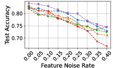
Attacks on features. To attack features, we inject random perturbation into the node features as in (Wu et al. 2020a). Firstly, we sample a noise matrix , where each entry in is sampled from the normal distribution . Then, we calculate reference amplitude , which is the mean of the maximal value of each node’s feature. We add Gaussian noise to the original feature matrix, and get the attacked feature matrix, where is the noise ratio. The results are reported in Figure 5. Again, HiD-Net consistently outperforms all other baselines under different perturbation rates by a margin for three datasets.
Non-over-smoothing with Increasing Steps
To demonstrate that our model solves the oversmoothing problem compared with other graph diffusion networks, we test different graph diffusion models with increasing propagation step from 2 to 20. Baselines include DGC, ADC and GRAND. The results are plotted in Figure 7. We can see that with the increase of , HiD-Net consistently performs better than other baselines.
Parameter Study
In this section, we investigate the sensitivity of parameters on all datasets.
Analysis of . We test the effect of in (16), and vary it from 0 to 1. From Figure 8(a) we can see that with the increase of , the performances of citation graphs rise first and then start to drop slowly, the performances of Chameleon and Squirrel have not changed too much, and the performance of Actor first rises and then remains unchanged. As citation graphs are more homophily, we need to focus less on the node itself, implying a small , while on heterophily graphs, we need to focus more on the node itself.
Analysis of . In order to check the impact of the diffusion term, we study the performance of HiD-Net with varying from 0 to 1. The results are shown in Figure 8(b). We can see that as the value of increases, the accuracies generally increase, while the accuracy on Actor remains relatively stable, implying that the features diffused from 1-hop and 2-hop neighbors are very informative.
Analysis of . Finally we test the effect of in (16) and vary it from 0 to 0.6. With the increase of , the accuracies on different datasets do not change much, so we just separately plot each dataset for a clearer illustration here. As can be seen in Figure 6, with the increase of , the performance on Cora and Chameleon rises first and then drops, and different graphs have different best choices of . The results on other datasets are shown in Appendix.
Conclusion
In this paper, we propose a generalized diffusion graph framework, which establishes the relation between diffusion equation with different GNNs. Our framework reveals that current graph diffusion networks mainly consider the first-order diffusion equation, then based on our finding of the monophily property of labels, we derive a novel high-order diffusion graph network (HiD-Net). HiD-Net is more robust and general on both homophily and heterophily graphs. Extensive experimental results verify the effectiveness of HiD-Net. One potential issue is that our model utilizes a constant diffusivity coefficient, and a future direction is to explore a learnable diffusivity coefficient depending on time and space. Our work formally points out the relation between diffusion equation with a wide variety of GNNs. Considering that previous GNNs are designed mainly based on spatial or spectral strategies, this new framework may open a new path to understanding and deriving novel GNNs. We believe that more insights from the research community on the diffusion process will hold great potential for the GNN community in the future.
Acknowledgments
This work is supported in part by the National Natural Science Foundation of China (No. U20B2045, 62192784, U22B2038, 62002029, 62172052, 62322203).
References
- Abu-El-Haija et al. (2019) Abu-El-Haija, S.; Perozzi, B.; Kapoor, A.; Alipourfard, N.; Lerman, K.; Harutyunyan, H.; Ver Steeg, G.; and Galstyan, A. 2019. Mixhop: Higher-order graph convolutional architectures via sparsified neighborhood mixing. In international conference on machine learning, 21–29. PMLR.
- Altenburger and Ugander (2018) Altenburger, K. M.; and Ugander, J. 2018. Monophily in social networks introduces similarity among friends-of-friends. Nature human behaviour, 2(4): 284–290.
- Bruna et al. (2013) Bruna, J.; Zaremba, W.; Szlam, A.; and LeCun, Y. 2013. Spectral networks and locally connected networks on graphs. arXiv preprint arXiv:1312.6203.
- Chamberlain et al. (2021) Chamberlain, B.; Rowbottom, J.; Gorinova, M. I.; Bronstein, M.; Webb, S.; and Rossi, E. 2021. Grand: Graph neural diffusion. In International Conference on Machine Learning, 1407–1418. PMLR.
- Chen, Wu, and Zaki (2020) Chen, Y.; Wu, L.; and Zaki, M. 2020. Iterative deep graph learning for graph neural networks: Better and robust node embeddings. Advances in Neural Information Processing Systems, 33: 19314–19326.
- Chung and Graham (1997) Chung, F. R.; and Graham, F. C. 1997. Spectral graph theory. 92. American Mathematical Soc.
- Defferrard, Bresson, and Vandergheynst (2016) Defferrard, M.; Bresson, X.; and Vandergheynst, P. 2016. Convolutional neural networks on graphs with fast localized spectral filtering. Advances in neural information processing systems, 29.
- Franceschi et al. (2019) Franceschi, L.; Niepert, M.; Pontil, M.; and He, X. 2019. Learning discrete structures for graph neural networks. In International conference on machine learning, 1972–1982. PMLR.
- Gao and Ji (2019) Gao, H.; and Ji, S. 2019. Graph u-nets. In international conference on machine learning, 2083–2092. PMLR.
- Hamilton, Ying, and Leskovec (2017) Hamilton, W.; Ying, Z.; and Leskovec, J. 2017. Inductive representation learning on large graphs. Advances in neural information processing systems, 30.
- Hu et al. (2020) Hu, W.; Fey, M.; Zitnik, M.; Dong, Y.; Ren, H.; Liu, B.; Catasta, M.; and Leskovec, J. 2020. Open graph benchmark: Datasets for machine learning on graphs. Advances in neural information processing systems, 33: 22118–22133.
- Kipf and Welling (2016a) Kipf, T. N.; and Welling, M. 2016a. Semi-supervised classification with graph convolutional networks. arXiv preprint arXiv:1609.02907.
- Kipf and Welling (2016b) Kipf, T. N.; and Welling, M. 2016b. Variational graph auto-encoders. arXiv preprint arXiv:1611.07308.
- Klicpera, Bojchevski, and Günnemann (2018) Klicpera, J.; Bojchevski, A.; and Günnemann, S. 2018. Predict then propagate: Graph neural networks meet personalized pagerank. arXiv preprint arXiv:1810.05997.
- Lei et al. (2022) Lei, R.; Wang, Z.; Li, Y.; Ding, B.; and Wei, Z. 2022. EvenNet: Ignoring Odd-Hop Neighbors Improves Robustness of Graph Neural Networks. In NeurIPS.
- Liu, Gao, and Ji (2020) Liu, M.; Gao, H.; and Ji, S. 2020. Towards deeper graph neural networks. In Proceedings of the 26th ACM SIGKDD international conference on knowledge discovery & data mining, 338–348.
- Liu et al. (2021) Liu, X.; Ding, J.; Jin, W.; Xu, H.; Ma, Y.; Liu, Z.; and Tang, J. 2021. Graph Neural Networks with Adaptive Residual. Advances in Neural Information Processing Systems, 34.
- Ma et al. (2021) Ma, Y.; Liu, X.; Zhao, T.; Liu, Y.; Tang, J.; and Shah, N. 2021. A unified view on graph neural networks as graph signal denoising. In Proceedings of the 30th ACM International Conference on Information & Knowledge Management, 1202–1211.
- Ouyang et al. (2023) Ouyang, R.; Elliott, A.; Limnios, S.; Cucuringu, M.; and Reinert, G. 2023. L2G2G: A Scalable Local-to-Global Network Embedding with Graph Autoencoders. In International Conference on Complex Networks and Their Applications, 400–412. Springer.
- Pei et al. (2020) Pei, H.; Wei, B.; Chang, K. C.-C.; Lei, Y.; and Yang, B. 2020. Geom-gcn: Geometric graph convolutional networks. arXiv preprint arXiv:2002.05287.
- Song et al. (2022) Song, Y.; Kang, Q.; Wang, S.; Kai, Z.; and Tay, W. P. 2022. On the robustness of graph neural diffusion to topology perturbations. arXiv preprint arXiv:2209.07754.
- Thorpe et al. (2022) Thorpe, M.; Nguyen, T. M.; Xia, H.; Strohmer, T.; Bertozzi, A.; Osher, S.; and Wang, B. 2022. GRAND++: Graph neural diffusion with a source term. In International Conference on Learning Representations.
- Veličković et al. (2017) Veličković, P.; Cucurull, G.; Casanova, A.; Romero, A.; Lio, P.; and Bengio, Y. 2017. Graph attention networks. arXiv preprint arXiv:1710.10903.
- Wang et al. (2017) Wang, X.; Cui, P.; Wang, J.; Pei, J.; Zhu, W.; and Yang, S. 2017. Community preserving network embedding. In Proceedings of the AAAI conference on artificial intelligence, volume 31.
- Wang et al. (2021) Wang, Y.; Wang, Y.; Yang, J.; and Lin, Z. 2021. Dissecting the diffusion process in linear graph convolutional networks. Advances in Neural Information Processing Systems, 34.
- Weickert (1998) Weickert, J. 1998. Anisotropic diffusion in image processing, volume 1. Teubner Stuttgart.
- Wu et al. (2019) Wu, F.; Souza, A.; Zhang, T.; Fifty, C.; Yu, T.; and Weinberger, K. 2019. Simplifying graph convolutional networks. In International conference on machine learning, 6861–6871. PMLR.
- Wu et al. (2020a) Wu, T.; Ren, H.; Li, P.; and Leskovec, J. 2020a. Graph information bottleneck. Advances in Neural Information Processing Systems, 33: 20437–20448.
- Wu et al. (2020b) Wu, Z.; Pan, S.; Chen, F.; Long, G.; Zhang, C.; and Philip, S. Y. 2020b. A comprehensive survey on graph neural networks. IEEE transactions on neural networks and learning systems, 32(1): 4–24.
- You, Ying, and Leskovec (2019) You, J.; Ying, R.; and Leskovec, J. 2019. Position-aware graph neural networks. In International Conference on Machine Learning, 7134–7143. PMLR.
- Yu et al. (2023) Yu, X.; Liu, Z.; Fang, Y.; and Zhang, X. 2023. Learning to count isomorphisms with graph neural networks. arXiv preprint arXiv:2302.03266.
- Zang and Wang (2020) Zang, C.; and Wang, F. 2020. Differential Deep Learning on Graphs and its Applications.
- Zhang et al. (2018) Zhang, M.; Cui, Z.; Neumann, M.; and Chen, Y. 2018. An end-to-end deep learning architecture for graph classification. In Thirty-second AAAI conference on artificial intelligence.
- Zhao et al. (2021) Zhao, J.; Dong, Y.; Ding, M.; Kharlamov, E.; and Tang, J. 2021. Adaptive Diffusion in Graph Neural Networks. Advances in Neural Information Processing Systems, 34.
- Zhou et al. (2020) Zhou, J.; Cui, G.; Hu, S.; Zhang, Z.; Yang, C.; Liu, Z.; Wang, L.; Li, C.; and Sun, M. 2020. Graph neural networks: A review of methods and applications. AI Open, 1: 57–81.
- Zhu et al. (2021) Zhu, M.; Wang, X.; Shi, C.; Ji, H.; and Cui, P. 2021. Interpreting and unifying graph neural networks with an optimization framework. In Proceedings of the Web Conference 2021, 1215–1226.
| Dataset | k | Hidden dimension | Learning rate | Weight Decay | dropout | ||||
|---|---|---|---|---|---|---|---|---|---|
| Cora | 0.1 | 0.9 | 0.3 | 0.8 | 10 | 128 | 0.01 | 0.00 | 0.55 |
| Citeseer | 0.1 | 0.9 | 0.2 | 0.6 | 10 | 64 | 0.005 | 0.05 | 0.5 |
| Pubmed | 0.08 | 0.92 | 0.3 | 1 | 8 | 32 | 0.02 | 0.0005 | 0.5 |
| Chameleon | 0.1 | 0.9 | 0.05 | 1 | 1 | 64 | 0.6 | 0.01 | 0.0005 |
| Squirrel | 0.1 | 0.9 | 0.3 | 1 | 1 | 64 | 0.02 | 0.0005 | 0.5 |
| Actor | 0.1 | 0.9 | 0.1 | 0.2 | 2 | 64 | 0.005 | 0.005 | 0.5 |
| ogbn-arxiv | 0.05 | 0.94 | 0.1 | 0.9 | 4 | 64 | 0.02 | 0.0005 | 0.5 |
Appendix A Proofs
Proof of Proposition 1
Graph Convolutional Network (GCN) has the following propagation mechanism which conducts linear transformation and nonlinearity activation repeatedly throughout layers:
| (20) |
where is the trainable weight matrix at layer . Simplifying Graph Convolutional Network (SGC) (Wu et al. 2019) removes nonlinearities and collapses weight matrices between consecutive layers, which has similar propagation mechanism with GCN and exhibits comparable performanceas. SGC propagates as:
| (21) |
where . We show that the propagation mode of SGC (GCN) is a special form of the generalized diffusion framework:
According to (9) we have:
| (22) |
With , on all nodes we have:
| (23) |
so
| (24) |
which matches the propagation mechanism of SGC.
Proof of Proposition 2.
PPNP is a graph neural network which utilizes a propagation scheme derived from personalized PageRank and adds a chance of teleporting back to the root node, which ensures that the PageRank score encodes the local neighborhood for every root node. PPNP’s model equation is:
| (25) |
and APPNP approximates PPNP via power iteration:
| (26) |
As stated in Remark 1, the steady state of (6) is (8). With , , and in (8), on all nodes, we have:
| (27) |
So
| (28) | ||||
which works the same as PPNP.
Proof of Proposition 3.
GAT (Veličković et al. 2017) is an attention-based architecture to perform node classification of graph-structured data. The attention coefficient between node and node is computed based on a shared attentional mechanism:
| (29) |
where is a shared attentional mechanism at time , and is the weight matrix.
As in (11), with , we have:
| (30) |
Let be the attention matrix at time , and is the element of it . With , on all nodes, we have
| (31) |
so,
| (32) |
which works as the propagation of GAT.
Proof of Proposition 4.
AMP (Liu et al. 2021) designs a better message passing scheme with node-wise adaptive feature aggregation and residual connection. With the normalized ajacency matrix, it propagates as:
| (33) |
where is the stepsize, and is the coefficient.
From (12), with we have:
| (34) | ||||
so
| (35) | ||||
which works as the propagation of AMP.
Proof of Proposition 5.
Deep Adaptive Graph Neural Networks (DAGNN) (Liu, Gao, and Ji 2020) adaptively incorporates information from large receptive fields. DAGNN propagates as:
| (36) | ||||
where are the learnable retainment coefficients and .
When , we have:
| (37) | ||||
as the propagation of DAGNN goes.
Proof of Proposition 6
Proof.
Clearly, for all for all
| (38) |
for all for all , assume that
| (39) |
Then, for all , we have
| (40) | ||||
as required.
∎
Proof of Proposition 7.
From (16), on all nodes, we have
| (41) | ||||
Then we have
| (42) |
where .
The resulting prediction at time is
| (43) |
Since , and is symmetrically normalized, we have , taking the limit the left term tends to 0 and the right term becomes a geometric series. Resulting in
| (44) | ||||
Proof of Proposition 8.
Firstly we assume that there exists and for all when , then and , so
| (45) | ||||
which contradict to the assumption. As , the features among neighbors are less likely to be similar, thus alleviating the oversmoothing issue.
Appendix B Reproducibility Information
| Dataset | Nodes | Edges | Classes | Features | Train/Val/Test nodes |
|---|---|---|---|---|---|
| Cora | 2,708 | 5,429 | 7 | 1,433 | 140/500/1,000 |
| Citeseer | 3,327 | 4,732 | 6 | 3,703 | 120/500/1,000 |
| Pubmed | 19,717 | 44,338 | 3 | 500 | 60/500/1,000 |
| ogbn-arxiv | 169,343 | 1,166,243 | 40 | 128 | 90941/29799/48603 |
| Chameleon | 2,277 | 36,101 | 5 | 2,325 | 1092/729/456 |
| Squirrel | 5,201 | 217,073 | 5 | 2,089 | 2496/1664/1041 |
| Actor | 7,600 | 33,544 | 5 | 931 | 3648/2432/1520 |
Datasets
The details of these datasets are summarized in Table 4.
Hyperparameters
We use a two-layer MLP as the model , following APPNP. For all models, we use the Adam optimizer and search the optimal learning rate over {0.005, 0.01, 0.02, 0.1, 0.6}, weight decay {0.0, 0.0005, 0.005, 0.01, 0.05}, hidden dimension {32, 64, 128}, dropout {0.0005, 0.1, 0.5, 0.55}, {1, 2, 4, 8, 10}, {0.2, 0.4, 0.6, 0.8, 0.9, 1}, {0.05, 0.08, 0.1}, {0.9, 0.92, 0.94}, .
The hyperparameters are shown in Table 3.
Environment
The environment where our code runs is shown as follows:
-
•
Operating system: Linux version 3.10.0-693.el7.x86_64
-
•
CPU information: Intel(R) Xeon(R) Silver 4210 CPU @ 2.20GHz
-
•
GPU information: GeForce RTX 3090
Other Source Code
The acquisition of all the code below complies with the provider’s license and do not contain personally identifiable information and offensive content. The address of code of baselines are listed as follows:
GCN (MIT license): https://github.com/tkipf/pygcn
GAT (MIT license): https://github.com/Diego999/pyGAT
APPNP (MIT license): https://github.com/klicperajo/ppnp
GRAND (MIT license): https://github.com/twitter-research/graph-neural-pde
ADC (MIT license): https://github.com/abcbdf/ADC
DGC (MIT license): https://github.com/yifeiwang77/dgc
Appendix C Time complexity
The propagation step of HiD-Net can be formulated as:HiD-Net can be formulated as:
As can be precomputed, it takes to calculate , where , is the number of the nodes, is the dimension of the feature vector. It takes to calculate , and to calculate and . So the time complexity of the propagation step of HiD-Net is and the first-order diffusion is also .
Appendix D More results
Analysis of parameter can be found in Figure 9.


Appendix E Comparision with other GNN models
We compare our model based on DMP with existing methods from the following four perspectives:
(1) Compared with existing discrete GNNs which capture two-hop connectivity (e.g., GCNs, GAT), our model is based on the diffusion equation which generalizes existing discrete GNNs to the continuous case, and the continuous GNNs are fundamentally different from discrete GNNs. The diffusion-based models have unique characteristics. For example, from the perspective of continuous graph diffusion, we can decouple the terminal time and the feature propagation steps, making it more flexible and capable of exploiting a very large number of feature propagation steps, so diffusion-based methods are able to address the common plights of graph learning models such as oversmoothing (Chamberlain et al. 2021; Wang et al. 2021). Moreover, the diffusion equation can be seen as partial differential equations (PDEs) (Chamberlain et al. 2021), thus introducing many schemes to solve the graph diffusion equation such as explicit scheme, implicit scheme, and multi-step scheme, some of which are more stable and converge faster than normal GNNs.
(2) Compared with the first-order diffusion process, HiD-Net utilizes the 2-hop neighbors’ information, where the advantages are: First, it considers a larger neighborhood size and captures the local environment around a node, thus even if there are some abnormal features among the 1-hop neighbors, their negative effect can still be alleviated. Second, the 2-hop neighbors provide an additional stronger correlation with labels according to the monophily property, so even if the 1-hop neighbors may be heterophily, HiD-Net can still make better predictions.
(3) Compared with the first-order diffusion process which captures high-order connectivity through iterative adjacent message passing, our proposed second-order diffusion equation is still very different from it. Specifically, the learned representation based on the first-order diffusion process after two propagation steps at time is:
| (46) | ||||
After one propagation step at time , HiD-Net has:
| (47) | |||
Here, in order to facilitate the analysis, we use , , to denote the coefficient of , and separately. By analyzing the proportions between different coefficients, we can analyze the weights of neighbors of different orders to see how flexible it is to adjust the balance between neighbors of different orders.
From (46), we have:
| (48) |
| (49) |
From (47) , we have:
| (50) |
| (51) |
According to (48), we can adjust the balance between the node itself and its neighbors by adjusting and . However, as and are fixed to adjust , we can’t adjust . That is to say, the proportion of first-order to second-order neighbors is fixed, so the first-order diffusion process can’t assign an appropriate proportion for first-order to second-order neighbors.
According to (50), we can change and to adjust the balance between the node itself and its neighbors. According to (51), we can adjust the balance between first-order neighbors and second-order neighbors by , thus breaking the limitation of the first-order diffusion process.
(4) Time and memory complexity comparison
The propagation step of the first-order and the second-order diffusion have the same memory complexity and time complexity. As can be precomputed, it takes to calculate , where , is the number of the nodes, is the dimension of the feature vector. It takes to calculate , and to calculate and . So the time complexity of the propagation step of HiD-Net is and the first-order diffusion is also . The memory cost of the first-order diffusion and the second-order diffusion propagation step is .