A generalization of Cardy’s and Schramm’s formulae

Percolation is an archetypical model of phase transition, used to describe many natural phenomena, from the spread of epidemics to a liquid seeping through a porous medium. It was introduced by Broadbent and Hammersley [1] but appeared even earlier in the problem section of the American Mathematical Monthly [20].

In the simplest setup of Bernoulli percolation, vertices (sites) or edges (bonds) of a graph are independently declared open or closed with probabilities $p$ and $1-p$ correspondingly; the resulting model is called site or bond percolation correspondingly. Connected clusters of open sites (or bonds) are then studied. For example, one can ask how the probability of having an open cluster connecting two sets depends on $p$. Despite simple formulation, the model approximates physical phenomena quite well and exhibits a very complicated behavior.

There is an extensive theory, see e.g. [5], but still there are many open questions. For instance, it is not known whether probability $\theta(p)$ of having an infinite open cluster containing origin in $\mathbb{Z}^{3}$ depends continuously on $p$.

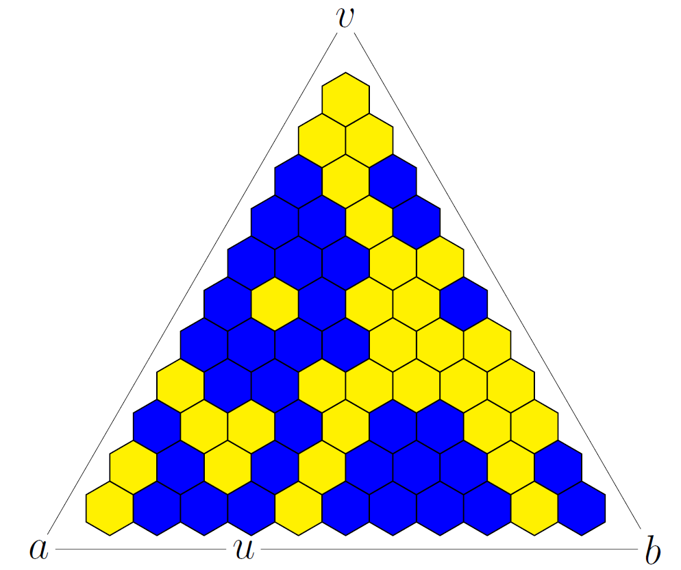
In contrast, planar models are fairly well understood. We will study critical site percolation on the triangular lattice, which by duality can be represented as a random coloring of faces (plaquettes) on the hexagonal lattice; see Figure 1, where open and closed hexagons are represented by blue and yellow colors. For this model, it is known that the critical value $p_{c}$ is equal to $1/2$, which was first proved by Kesten using duality; see [5]. This means in particular that when one takes a topological rectangle (i.e. a domain with four marked boundary points) and superimposes a mesh $\delta$ lattice, the crossing probability (i.e. the probability of the existence of an open crossing between the chosen opposite sides) tends to $0$ when $p<p_{c}$ and to $1$ when $p>p_{c}$ as $\delta\searrow 0$. The same argument shows that for $p=p_{c}$ the crossing probability is nontrivial, and in 1992 physicist J. Cardy suggested an exact formula for its scaling limit as $\delta\searrow 0$ as a hypergeometric function of the conformal modulus (see Corollary 2.3). The formula is expected to hold for any critical percolation, but so far it was proved only for the model under consideration by the third author [16, 18, 9] by establishing discrete holomorphicity of certain observables.

Henceforth one can connect [17] scaling limits of percolation interfaces between open and closed clusters to Schramm’s SLE(6) curve [13, 14] and deduce many properties, e.g. the values of critical exponents and dimensions [19].

This leaves open the question of how far one can go with purely discrete techniques. For example, in the critical Ising model much can be learned from similar observables without alluding to SLE [6, 3], as is the case for the Uniform Spanning Tree [7, §11.2]. Cf. an elementary example in [12].

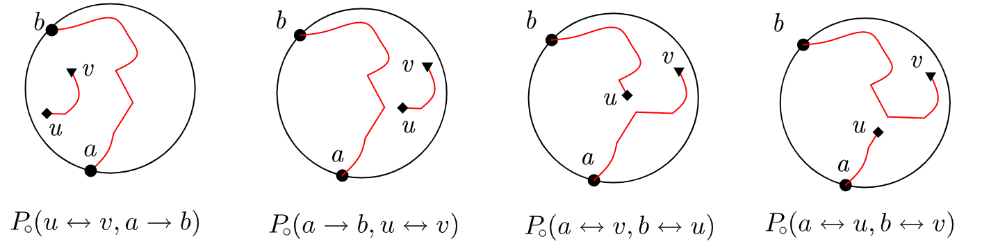
In this paper, we introduce a new percolation observable, which allows us to prove new results and give new proofs to old ones, which beforehand required an SLE limit (see Corollary 2.4). In particular, we find the difference of the probabilities of having a percolation interface to the right and to the left of two given points in the scaling limit (see Figure 2 and Theorem 2.1).

Remarkably, the observable we introduce here is nothing more than a natural generalization of the observable from [9] which itself is just equal to the observable from [16]. However, it seems that getting to the new observable directly from [16] was not as straightforward (and so took a while). It is worth noting that our construction admits further generalizations, at least to the problem with six disorders instead of four [8] and that some appearing functions bear resemblance to modular forms discussed by P. Kleban and D. Zagier [10].

Organization of the paper. In §2 and §3 we state main and auxiliary results respectively. In §4 and Appendix A we prove conceptual and technical ones respectively.

Let us introduce a few definitions to state our result precisely (see Figure 2).

Consider a hexagonal lattice on the complex plane $\mathbb{C}$ formed by hexagons with side $\delta$. Let $\Omega\subset\mathbb{C}$ be a domain bounded by a closed smooth curve (that is, $\partial\Omega$ is the image of a periodic $C^{1}$ map $\mathbb{R}\to\mathbb{C}$ with nonzero derivative). A lattice approximation of the domain $\Omega$ is the maximal-area connected component $\Omega^{\delta}$ of the union of all the hexagons lying inside $\Omega$ (if such a connected component is not unique, then we choose any of them). Mark two distinct boundary points $a,b\in\partial\Omega$ and two other points $u,v\in\overline{\Omega}:=\Omega\cup\partial\Omega$. Their lattice approximations are the midpoints $a^{\delta},b^{\delta},u^{\delta},v^{\delta}$ of sides of the hexagons of $\Omega^{\delta}$, closest to $a,b,u,v$ respectively (if the closest midpoint is not unique, then we choose any of them). Clearly, $a^{\delta},b^{\delta}\in\partial\Omega^{\delta}$. We allow $u^{\delta}=v^{\delta}$ but disallow the coincidence of any other pair among $a^{\delta},b^{\delta},u^{\delta},v^{\delta}$.

The percolation model on $\Omega^{\delta}$ is the uniform measure on the set of all the colorings of hexagons of $\Omega^{\delta}$ in two colors, say, blue and yellow. Introduce the Dobrushin boundary condition: in addition, paint the hexagons outside $\Omega^{\delta}$ bordering upon the clockwise arc of $\partial\Omega^{\delta}$ between $a^{\delta}$ and $b^{\delta}$ blue, and the ones bordering upon the counterclockwise arc yellow (the ones bordering upon $a^{\delta}$ and $b^{\delta}$ are paint both colors). For the whole coloring, the interface $a^{\delta}b^{\delta}$ is the oriented simple broken line going from $a^{\delta}$ to $b^{\delta}$ along the sides of the hexagons of $\Omega^{\delta}$ such that all the hexagons bordering upon $a^{\delta}b^{\delta}$ from the left are blue and all the hexagons bordering upon $a^{\delta}b^{\delta}$ from the right are yellow.

The interface $a^{\delta}b^{\delta}$ splits the union of the sides of the hexagons of $\Omega^{\delta}$ into connected components. Let $P(u^{\delta}\cdots v^{\delta},a^{\delta}\rightarrow b^{\delta})$ (respectively, $P(a^{\delta}\rightarrow b^{\delta},u^{\delta}\cdots v^{\delta})$) be the probability that $u^{\delta}$ and $v^{\delta}$ belong to the same component lying to the left (respectively, to the right) from $a^{\delta}b^{\delta}$.

Our main result expresses those probabilities in terms of certain conformal mappings. Let $\psi$ be a conformal mapping of $\Omega$ onto the upper half-plane $\{z:\mathrm{Im}\,z>0\}$ (continuously extended to $\overline{\Omega}$) taking $a$ and $b$ to $0$ and $\infty$ respectively. Let $g$ be the conformal mapping of $\mathbb{C}-(-\infty;-1]\cup[1;+\infty)$ onto the interior of the rhombus with the vertices $\pm 1,\pm i\sqrt{3}$, continuously extended to the points $\pm 1$ and having fixed points $0,+1,-1$. See Figure 3.

Here if both $u$ and $v$ belong to the counterclockwise (respectively, clockwise) boundary arc $ab$ of $\partial\Omega$, then the value of the mapping $g$ in (1) is understood as continuously extended from the lower (respectively, upper) half-plane. There is an explicit formula for the mapping $g$.

Hereafter

denotes the principal branch of the hypergeometric function in $\mathbb{C}-[1,+\infty)$; [11, Ch. V, §7].

While the proof of Theorem 2.1 is similar to the proof of Cardy’s formula from [9], the proof of Schramm’s formula by means of Theorem 2.1 is essentially new, and we think is simpler than the original one. Originally, Schramm’s formula was stated as a corollary of the weak convergence of interfaces to SLE(6), itself deduced from Cardy’s formula [16]; but actually, it is rather technical to deduce the convergence of surrounding probabilities from the latter weak convergence.

Theorem 2.1 is deduced from a more general result, interesting in itself. Let us introduce some notation, state the main result in full strength, and state lemmas used in the proof, giving proofs in the next sections. Throughout this section we assume that the assumptions of Theorem 2.1 hold, we omit the superscript $\delta$ so that $a,b,u,v$ mean $a^{\delta},b^{\delta},u^{\delta},v^{\delta}$ respectively (everywhere except Theorem 3.2, Lemmas 3.8–3.9, and other explicitly indicated places), and assume that $a,b,u,v$ are pairwise distinct. Remarkably, although we take $u=v$ in the proof of Schramm’s formula at the very end, here we need $u\neq v$.

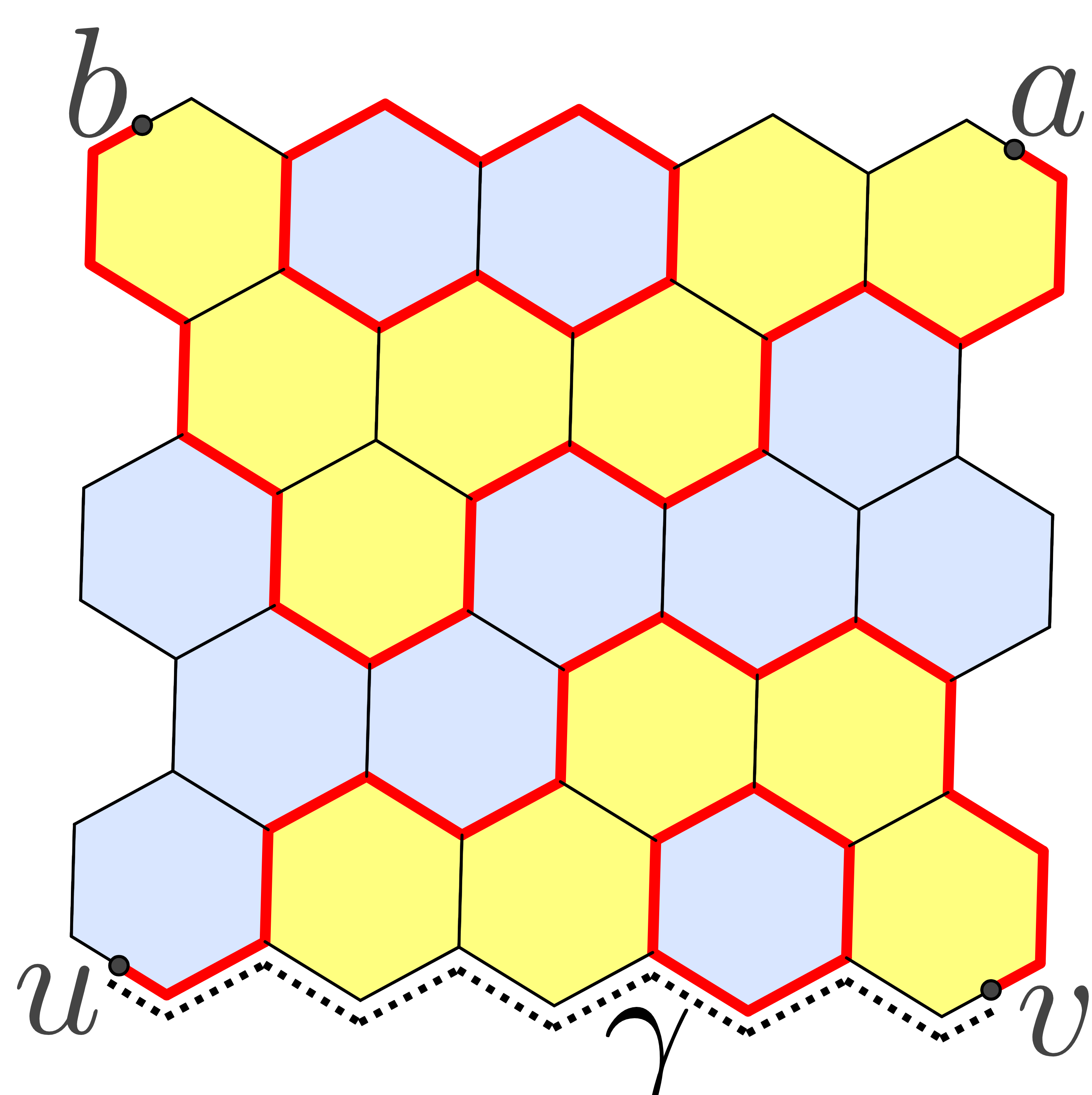
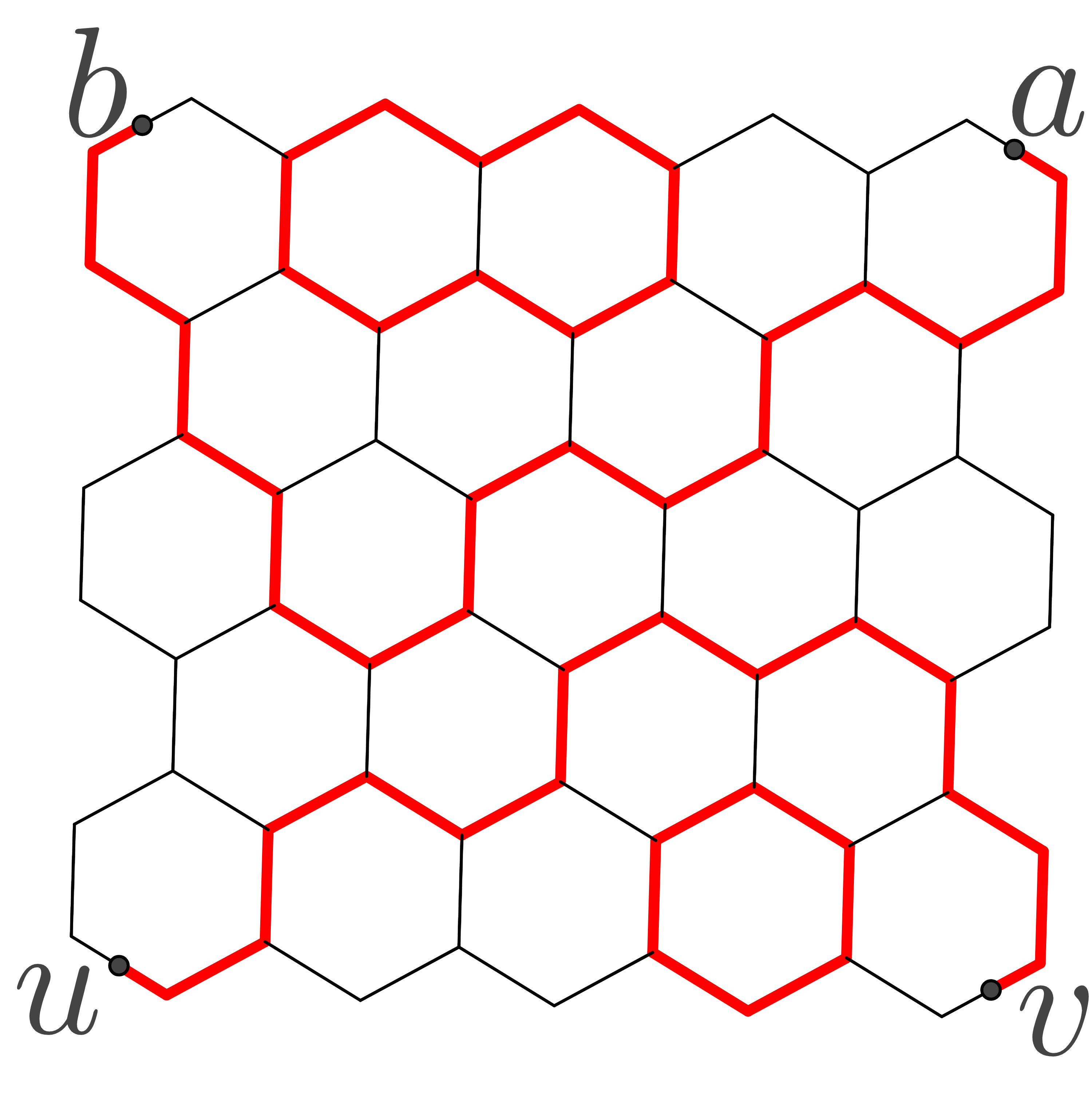
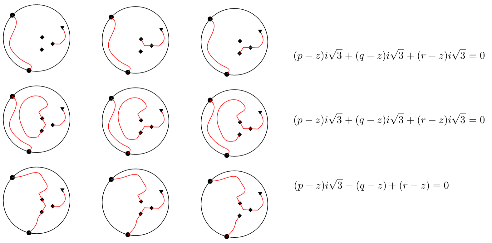
In what follows a hexagon is a hexagon of the lattice approximation $\Omega^{\delta}$. A midpoint is a midpoint of a side of a hexagon. A half-side is a segment joining a midpoint with an endpoint of the same side. A broken line is a simple broken line (possibly closed) consisting of half-sides, viewed as a subset of the plane. A broken line $pq$ is such a broken line with distinct endpoints $p$ and $q$. A loop configuration with disorders at $a,b,u,v$ (or just loop configuration for brevity) is a disjoint union of several broken lines, with exactly two being non-closed and having the endpoints at $a,b,u,v$ and all the other ones being closed. It is easy to see (see, for instance, [9, §1.2]) that the number of loop configurations equals the number of colorings of hexagons in two colors. See Figure 4.

Denote by $P_{\!\!\circ}(a\leftrightarrow u,b\leftrightarrow v)$ the fraction of loop configurations containing a broken line $au$ (and hence another broken line $bv$ as well). Define $P_{\!\!\circ}(a\leftrightarrow v,b\leftrightarrow u)$ analogously. See Figure 5.

Now consider loop configurations containing a broken line $ab$. The broken line (which we always orient from $a$ to $b$) divides the polygon $\Omega^{\delta}$ into connected components, each bordering upon $ab$ either from the right or from the left. We say that those connected components lie to the right and to the left from $ab$ respectively. Denote by $P_{\!\!\circ}(a\rightarrow b,u\leftrightarrow v)$ the fraction of loop configurations containing broken lines $ab$ and $uv$ such that $uv$ lies to the right from $ab$. Define $P_{\!\!\circ}(u\leftrightarrow v,a\rightarrow b)$ analogously. Beware the different meaning of notations $P_{\!\!\circ}(a\leftrightarrow v,b\leftrightarrow u)$ and $P_{\!\!\circ}(u\leftrightarrow v,a\rightarrow b)$.

We have decomposed the set of all loop configurations into $4$ subsets (called link patterns) depending on the arrangement of broken lines with the endpoints $a,b,u,v$ (see Figure 5).

The parafermionic observable is the complex-valued function on the set of pairs of midpoints, distinct from $a$ and $b$, given by the formula

The following lemma and theorem, being the main result in full strength, will imply Theorem 2.1.

The latter automatically holds for $u=v$ as well.

The proof of this theorem uses the following properties of the parafermionic observable.

Denote by $[z;w]$ the straight-line segment with the endpoints $z,w\in\mathbb{C}$.

By the inradius of a closed bounded domain $(\overline{\Omega},a,b,c)$ with three marked points we mean the minimal radius of a disk $D$ such that no two points among $a,b,c$ belong to the same connected component of $\overline{\Omega}-D$. For instance, if $\overline{\Omega}$ is the triangle with the vertices $a,b,c$ then the inradius of $(\overline{\Omega},a,b,c)$ equals the usual inradius of the triangle, i.e. the radius of the inscribed circle. We are going to apply the following two lemmas to $c=v$.

All the assertions stated above are proved in the next section, except for Proposition 2.2 and the latter three technical lemmas proved in the appendix. The proof of Lemma 3.7 is completely analogous to [9, Lemma 10]; the other proofs in the appendix are obtained by well-known methods.

Let us show that Cardy’s and Schramm’s formulae are indeed particular cases of this result.

References

- [1] S. Broadbent, J. Hammersley, Percolation processes: I. Crystals and mazes. Math. Proc. Camb. Philos. Soc. 53:3 (1957) 629–641.
- [2] J.L. Cardy. Critical percolation in finite geometries, J. Phys. A, 25(4):L201–L206, 1992.
- [3] D. Chelkak, C. Hongler, K. Izyurov, Conformal invariance of spin correlations in the planar Ising model, Ann. Math. (2015), 1087–1138.
- [4] H. Duminil-Copin, Parafermionic observables and their applications to planar statistical physics models, volume 25 of Ensaios Mateáticos [Mathematical Surveys]. Sociedade Brasileira de Matemática, Rio de Janeiro, 2013.
- [5] G. Grimmett, Percolation, Vol. 321 of Grundlehren der Mathematischen Wissenschaften [Fundamental Principles of Mathematical Sciences]. Springer-Verlag, Berlin, second edition, 1999.
- [6] C. Hongler and S. Smirnov, The energy density in the planar Ising model, Acta Math., 211:2 (2013) 191–225.
- [7] R. Kenyon, Spanning forests and the vector bundle Laplacian, Ann. Prob. 39:5 (2011) 1983–2017.
- [8] M. Khristoforov and V. Kleptsyn, Smirnov’s observable and link pattern probabilities in percolation, in preparation.
- [9] M. Khristoforov, S. Smirnov, Percolation and O(1) loop model, preprint, 2021, \urlhttps://arxiv.org/abs/2111.15612.
- [10] P. Kleban, D. Zagier, Crossing probabilities and modular forms, J. Stat. Phys. 113 (2003) 431–454.
- [11] Z. Nehari, Conformal mapping, New York: Dover Publications, 1975.
- [12] I. Novikov, Percolation of three fluids on a honeycomb lattice, Monatsh Math 199, 611-626 (2022), \urlhttps://arxiv.org/abs/1912.01757.
- [13] O. Schramm, Scaling limits of loop-erased random walks and uniform spanning trees, Isr. J. Math. 118 (2000), 221–288. \urlhttps://arxiv.org/abs/math/9904022
- [14] O. Schramm, A percolation formula, Electron. Comm. Probab. 6 (2001) 115–120.
- [15] S. Sheffield and D.B. Wilson, Schramm’s proof of Watts’ formula, Ann. Probab. 39:5 (2011), Memorial Issue for Oded Schramm 1961–2008, 1844–1863.
- [16] S. Smirnov, Critical percolation in the plane: Conformal invariance, Cardy’s formula, scaling limits. C. R. Math. Acad. Sci. Paris, 333(3):239-244, 2001.
- [17] S. Smirnov, Critical percolation and conformal invariance. In: XIVth International Congress on Mathematical Physics: Lisbon, 2003.
- [18] S. Smirnov, Critical percolation in the plane, 2009, \urlhttps://arxiv.org/abs/0909.4499.
- [19] S. Smirnov, W. Werner, Critical exponents for two-dimensional percolation, Math. Res. Lett. 8:6 (2001), 729–744.
- [20] De Volson Wood, Problem, Amer. Math. Monthly 1 (1894), p. 99.
Mikhail Khristoforov
Saint Petersburg University
mikhail.khristoforov @ gmailcom
Mikhail Skopenkov
King Abdullah University of Science and Technology &
HSE University (Faculty of Mathematics) &
Institute for Information Transmission Problems of the Russian Academy of Sciences
mikhail.skopenkov @ gmailcom \urlhttps://users.mccme.ru/mskopenkov/
Stanislav Smirnov
Université de Genève, Genève 4, Switzerland &
&
Skolkovo Institute of Science and Technology
[email protected]