A GCICA Grant-Free Random Access Scheme for M2M Communications in Crowded Massive MIMO Systems
Abstract
A high success rate of grant-free random access scheme is proposed to support massive access for machine-to-machine communications in massive multiple-input multiple-output systems. This scheme allows active user equipments (UEs) to transmit their modulated uplink messages along with super pilots consisting of multiple sub-pilots to a base station (BS). Then, the BS performs channel state information (CSI) estimation and uplink message decoding by utilizing a proposed graph combined clustering independent component analysis (GCICA) decoding algorithm, and then employs the estimated CSIs to detect active UEs by utilizing the characteristic of asymptotic favorable propagation of massive MIMO channel. We call this proposed scheme as GCICA based random access (GCICA-RA) scheme. We analyze the successful access probability, missed detection probability, and uplink throughput of the GCICA-RA scheme. Numerical results show that, the GCICA-RA scheme significantly improves the successful access probability and uplink throughput, decreases missed detection probability, and provides low CSI estimation error at the same time.
Index Terms:
Grant-free random access, independent component analysis (ICA), massive MIMO, M2M communications.I Introduction
THE machine-to-machine (M2M) communications are centered on the intelligent interaction of user equipments (UEs) without human intervention, which is the enabler for the Internet of Things (IoT) to achieve the envision of the “Internet of Everything” [1, 2, 3, 4]. In recent years, M2M communications develop rapidly and have been applied to many scenarios, such as smart medical, smart vehicle, smart logistics, etc. Cisco visual networking index and forecast predicts that there will be around 28.5 billion connected UEs by 2022 [5]. The massive multiple-input multiple-output (MIMO) technology, which achieves significant improvements in energy and spectral efficiency and can serve massive UEs in the same time-frequency resource, is well suited for M2M communications [6, 7, 8].
For M2M communications in massive MIMO systems, random access procedure is a critical step to initiate a data transmission [9, 10]. Since payload data is usually in small size and the number of UEs in a cell is envisioned in the order of hundreds or thousands in M2M communications [11], random access procedure utilized in the long term evolution (LTE) network may induce excessive signaling overhead and cannot support massive access [9, 12].
Researchers are exploring new random access schemes for M2M communications in massive MIMO systems, and the grant-based random access schemes have been proposed in recent years. E. Björnson et al. proposed a strongest-user collision resolution (SUCRe) scheme, which allocates pilots to active UEs with largest channel gain among the contenders [13]. However, the number of successful accessing UEs decreases with the increase of the number of contenders [14]. To improve the pilot resource utilization of the SUCRe scheme, SUCR combined idle pilots access (SUCR-IPA) scheme was proposed in [15], where the weaker UEs randomly select idle pilots to increase the number of successful accessing UEs. A user identity-aided pilot access scheme was proposed for massive MIMO with interleave-division multiple-access systems, where the interleaver of each UE is available at the BS according to the one-to-one correspondence between UE’s identity number (ID) and its interleaver [16]. However, since the grant-based random access schemes require two handshake processes between the base station (BS) and UEs, considering the small packet transmission in M2M communication, such kind of random access scheme will introduce heavy signaling overhead and low data transmission efficiency.
To address this problem, the grant-free random access schemes have attracted much attention in recent years, which allow active UEs to transmit their pilots and uplink messages to the BS directly and perform activity detection, channel state information (CSI) estimation, and uplink message decoding in one shot. J. Ahn et al. proposed a Bayesian based random access scheme to detect the UE’s activity and estimate the CSI jointly by utilizing the expectation propagation algorithm, considering the BS with one antenna [17]. L. Liu et al. proposed a approximate message passing (AMP) based grant-free scheme to achieve the joint activity detection and CSI estimation for massive MIMO systems [18]. However, this AMP-based grant-free random access scheme requires long pilot sequence to achieve better performance, resulting in heavy pilot overhead. To support massive connectivity with low access delay and overhead, a novel grant-free random access scheme was proposed to detect active UEs and uplink message without CSI estimation in one shot [19]. However, the CSI estimation is needed for some M2M traffics for downlink beamforming in the case of time-division duplex (TDD) model, such as the telemedicine surgery requiring the downlink control signal transmission. The above-mentioned grant-free random access schemes consider the single pilot structure. Jiang et al. proposed to concatenate multiple orthogonal sub-pilots into a super pilot sequence, and the super pilot sequence is utilized for activity detection and CSI estimation [20]. Simulation results show that, compared to the single pilot structure, this super pilot structure can improve the number of successful UEs by utilizing their proposed detection approach. However, with the increase of the number of active UEs, the probability that more UEs have the same super pilot sequence increases, resulting in low row rank pilot selection matrix and thus degrading the number of successful UEs. This motivates interesting researches on how to support massive access by utilizing the super pilot structure.
To achieve this goal, we propose a graph combined clustering independent component analysis based random access (GCICA-RA) scheme. This scheme utilizes the super pilot structure and mainly consists of two steps. During the first step, all the active UEs concatenate their randomly selected sub-pilots to obtain their super pilot sequences, and send their super pilot sequences and modulated uplink messages to the BS. During the second step, the BS performs CSI estimation and uplink message decoding jointly by utilizing a proposed GCICA decoding algorithm, employs the estimated CSIs to detect active UEs by utilizing the characteristic of asymptotic favorable propagation of massive MIMO channel, and sends random access response (RAR) to active UEs. We analyze the successful access probability, missed detection probability, and uplink throughput of the GCICA-RA scheme. Numerical results show that, compared to the random access scheme proposed in [20], the GCICA-RA scheme significantly improves the successful access probability and uplink throughput, decreases missed detection probability, and provides low CSI estimation error at the same time.
The main contributions of this paper are summarized as follows.
-
•
We propose a GCICA algorithm to perform CSIs estimation and uplink message decoding jointly. Specifically, based on the received sub-pilot signal, the BS first utilizes a successive interference cancellation (SIC) algorithm to estimate CSIs of active UEs, and then decodes the uplink message by utilizing the estimated CSIs. Then, the BS utilizes a proposed CICA algorithm to decode uplink message and estimate CSIs of UEs whose CSIs cannot be estimated by the SIC algorithm. Simulation results show that, compared to the detection method proposed in [20], the number of successful UEs can be improved even multiple UEs having the same super pilot sequence.
-
•
For the SIC algorithm, we propose to employ the estimated CSIs without other overhead to find edges connecting to a recovered variable node, by utilizing the asymptotic favorable propagation of massive MIMO systems. This is different from the existing method where indexes of selected pilots should be inserted into the uplink message to find edges connected to a recovered variable node [14], which degrades data transmission efficiency.
-
•
We analyze the upper bound for the successful access probability and uplink throughput of the proposed GCICA-RA scheme, and derive the lower bound for the missed detection probability of the proposed GCICA-RA scheme.
The remainder of this paper is organized as follows. Section II introduces system model and the proposed GCICA-RA scheme. Section III describes SIC and CICA algorithms in the the proposed GCICA-RA scheme. We present the performance analysis in Section IV. Simulation results and the conclusion are given in Section V and VI, respectively.
Notations utilized throughout this paper are described in Table I.
| Notations | Description | ||
|---|---|---|---|
| Italic letters | Scalars | ||
| Boldface lower-case | Vectors | ||
| Boldface upper-case letters | Matrices | ||
| and |
|
||
| ‘*’ | Complex conjugate of a vector or a matrix | ||
| The element of a vector | |||
| The set of all real numbers | |||
|
|||
| The Euclidean norm of a vector | |||
| The cardinality of a set | |||
| arg() | The phase of complex | ||
| The rounding operation | |||
| The element of vector | |||
| The column of matrix |
II SYSTEM MODEL and The proposed GCICA-RA Scheme
II-A SYSTEM MODEL
In this paper, we consider massive MIMO communication systems in time-division duplex (TDD) mode. There is a BS with antennas and single-antenna UEs in a cell, where the number of active UEs in a random access procedure is .
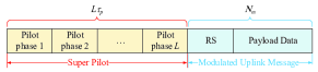
In the proposed GCICA-RA scheme, each UE transmits its modulated uplink message and super pilot to the BS directly. The BS performs CSI estimation and uplink message decoding by utilizing a proposed GCICA decoding algorithm, and then employs the estimated CSIs to detect active UEs. The frame structure of the GCICA-RA scheme is shown in Fig. 1. Specifically, the super pilot of each UE consists of consecutive sub-pilots, and the symbol length of each sub-pilot is . Therefore, the symbol length of each super pilot is . In addition, the proposed GCICA decoding algorithm utilizes multiple ICA classifiers to separate source signals. However, the phase of the separated signals is unpredictable.
To solve this problem, each active UE inserts a reference symbol (termed RS) with symbol length 1 into its uplink message [19]. Let denote the modulated uplink message of UE , where represents the symbol length of the modulated uplink message. Then, , represent the RS and the payload data with symbol length , respectively. Furthermore, since any complex symbol can be represented as a real symbol [21], we employ the BPSK modulation scheme in the proposed GCICA-RA scheme, i.e. .

II-B GCICA-RA scheme description
As shown in Fig. 2, the proposed GCICA-RA scheme allows each UE to transmit its modulated uplink message and super pilot to the BS directly. Then, the BS performs CSI estimation and uplink message decoding by utilizing a proposed GCICA decoding algorithm, employs the estimated CSIs to detect active UEs, and sends RAR information to active UEs. In addition, the proposed GCICA decoding algorithm first utilizes a SIC algorithm to estimate CSIs and decode the uplink message of active UEs, performs the number of active UEs estimation, and utilizes a proposed CICA algorithm to decode uplink messages and estimate CSIs of active UEs whose CSIs cannot be recovered by the SIC algorithm. The details are described as follows.
II-B1 Step 1: Super pilot and modulated uplink message transmission
There are sub-pilot phases, and each active UE randomly selects its sub-pilot from a set of mutually orthogonal normalized pilots during each sub-pilot phase. Concatenating these randomly selected sub-pilot sequences, each active UE obtains its super pilot. Following the frame structure as shown in Fig. 1, each active UE sends it super pilot and modulated uplink message to the BS. In addition, the value of RS is the same for all active UEs, and we set the RS to be 1, i.e., .
Then, let denote the independent and identically distributed (i.i.d.) small-scale fading channel from UE to the BS, i.e., . Let denote UE ’s transmitting power. Let stand for the channel gain between UE and the BS, which can be known for UE before the random access procedure [13]. Then, the received sub-pilot signal during the sub-pilot phase at the BS is
| (1) |
where stands for the set of UEs that select pilot during the sub-pilot phase, denotes the additive white noise matrix with each element following from a distribution of . In this paper, with different subscripts or superscripts will follow the same distribution. In addition, we consider to make the received signal from all active UEs have the same power [22].
The received superimposed uplink message at the BS is
| (2) |
II-B2 CSI estimation, uplink message decoding, active UE detection and RAR transmission
Based on the received sub-pilot signal and the superimposed uplink message, the BS performs CSI estimation and uplink message decoding jointly, and active UE detection and RAR information transmission. The details are described as follows.
CSI estimation and uplink message decoding
The BS utilizes the proposed GCICA decoding algorithm to perform CSI estimation and uplink message decoding. The details of the GCICA decoding algorithm are described as follows.
The BS first estimates the CSI corresponding to pilot during the sub-pilot phase by utilizing least squares (LS) method, denoted by
| (3) |
It can be seen from (3) that, during the sub-pilot phase, the estimated CSI corresponding to pilot is the sum of CSIs of active UEs selecting pilot . So, considering all sub-pilot phases, a bipartite graph can be used to describe the proposed GCICA-RA scheme, and thus the SIC algorithm can be utilized to estimate UEs’ CSIs on the bipartite graph. The procedure of the SIC algorithm is described in Section III-A in detail. We use to denote the estimated CSIs via the SIC algorithm, where is the number of estimated CSIs via the SIC algorithm. Thus, the detected uplink message can be obtained by utilizing LS method
| (4) |
After demodulating and decoding the detected uplink message , we obtain the corresponding decoded uplink message .
Then, based on the estimated CSIs corresponding to all pilots during the sub-pilot phase, the BS estimates the number of active UEs by utilizing the estimation method proposed in [19], denoted by , which is given by
| (5) |
We can observe from (5) that approaches with large . Therefore, the estimated number of active UEs whose CSIs cannot be obtained via the SIC algorithm is
| (6) |
Finally, by utilizing , , and , the BS employs a proposed CICA algorithm to obtain the CSIs and decoded uplink message of active UEs whose CSIs cannot be obtained via the SIC algorithm, denoted by and , respectively. The details of the CICA algorithm are descried in Section III-B.
Active UE detection and RAR information transmission
The BS detects an active UE by judging whether its CSI can be estimated (i.e., whether the corresponding estimated CSI is a valid CSI estimation), and this UE realizes whether it has been detected by the BS in a distributed manner. The details are described as follows.
We utilize to denote the estimated CSIs, and assume that is a valid CSI estimation. More specifically, is the estimated CSI for UE (i.e., , where denotes the estimation error and takes small values). By correlating with the estimated CSI corresponding to pilot during the sub-pilot phase (i.e., ), we have
| (7) | ||||
where (a) follows from the fact that, when goes into infinity, terms , by utilizing the asymptotic favorable propagation of massive MIMO channel, term is close to since elements in are small values, and (b) is derived based on the random matrix theory. In addition, it is easy to derive that, when is not a valid CSI estimation, is close to 0 by utilizing the random matrix theory. Therefore, the BS utilizes the following rule to judge whether is a valid CSI estimation: for the sub-pilot phase, if there only exits an element in set close to 1, is a valid CSI estimation because each active UE only selects one pilot during each sub-pilot phase; otherwise, is not a valid CSI estimation.
After obtaining all valid CSIs, the BS generates and broadcasts the RAR information to all active UEs where stands for the index set of valid CSI estimations.
The received RAR at UE is
| (8) |
Then, we have
| (9) |
where (a) is derived by utilizing the asymptotic favorable propagation of massive MIMO channel, similar to (7). Based on the value of , UE can realize whether it has been detected. If not, UE will reattempt the random access procedure in the upcoming random access slot.
III SIC and CICA algorithms
III-A SIC Algorithm
As we described in Section II-B, a bipartite graph can be used to describe the proposed GCICA-RA scheme, and thus the SIC algorithm can be utilized to estimate UEs’ CSIs on the bipartite graph. In this subsection, we first present the bipartite graph representation, and then describe the SIC algorithm in detail.
III-A1 Bipartite Graph Representation
A bipartite graph consists of variable nodes, factor nodes, and edges connecting variable nodes and factor nodes. We utilize active UEs and available pilots during each sub-pilot phase to represent variable nodes and factor nodes, respectively. Furthermore, if pilot is selected by UE during sub-pilot phase , we use to denote the corresponding factor node, and there exists an edge connecting the variable node with the factor node . The CSI of UE is marked on edges connected to UE . Note that, since we use the power control mechanism to make , we only need to estimate the small-scale fading channel. So, we only mark the small-scale fading coefficients between the BS and active UE. Furthermore, the degree of a node is referred to the number of edges connected to this node.
Example: Fig. 3(a) illustrates a bipartite graph based on 5 active UEs, 2 sub-pilot phases, and 3 available pilots. During each sub-pilot phase, active UEs (represented by circles) are variable nodes and all available pilots (represented by squares) are factor nodes. Since UE 1 and UE 2 select pilot during sub-pilot phase , UE 1 and UE 2 are connected to factor node by a black solid line. Since UE 3 selects pilot during sub-pilot phase , UE 3 is connected to factor node by a black solid line. Since UE 4 and UE 5 select pilot during sub-pilot phase , UE 4 and UE 5 are connected to factor node by a black solid line. Since UE 1 and UE 3 select pilot during sub-pilot phase , UE 1 and UE 3 are connected to factor node by a black solid line. Since UE 2, UE 4, and UE 5 all select pilot during sub-pilot phase , UE 2, UE 4 and UE 5 are connected to factor node by a black solid line.

III-A2 SIC Algorithm
The BS employs SIC algorithm to estimate UE’s CSI on the bipartite graph, and then utilizes the estimated CSIs to decode the uplink message. In the following, we briefly discuss the SIC algorithm, present the pseudo-code of the SIC algorithm in Algorithm 1, and give an example to show the SIC algorithm intuitively.
By performing the autocorrelation operation on CSI corresponding to each pilot during each sub-pilot phase, we have
| (10) | ||||
where (a) can be easily derived by utilizing the characteristic of asymptotic favorable propagation of massive MIMO channel.
(10) shows that, with large , approaches the number of active UEs selecting pilot during the sub-pilot phase. In other words, represents the degree of factor node .
During the first SIC iteration, the BS first finds factor nodes with degree 1 by utilizing (10). A factor node with degree 1 indicates that there is only one UE selecting the corresponding sub-pilot and the corresponding CSI can be recovered. Then, the BS finds other selected sub-pilots of UEs whose CSIs are recovered. More specifically, for each CSI corresponding to factor node with degree larger than 1, after subtracting each recovered CSI, the BS utilizes (10) to compute the new degree of this factor node. If the new degree is less than the previous degree, this means that the sub-pilot corresponding to this factor node is selected by active UE corresponding to this recovered CSI. We subtract the recovered CSI from the CSI corresponding to this factor node and update the new degree as the previous degree of this factor node. This is equivalent to delete the edges between this active UE and its selected sub-pilots on the bipartite graph. Thus, a new bipartite graph can be obtained, and SIC iteration continues until there is no factor node with degree 1.
Since each active UE selects its sub-pilots randomly, there exits the case of UE having no pilot collision during multiple sub-pilot phases. This results in the case of the recovered multiple CSIs corresponding to the same UE. Luckily, by utilizing the asymptotic favorable propagation of massive MIMO channel, we can find these CSIs from the recovered CSIs and select one of them as the recovered CSI of this UE. For example, if estimated and correspond to the same active UE, by utilizing the asymptotic favorable propagation of massive MIMO channel, is close to 1 with large . Otherwise, is close to 0 with large . Finally, the recovered CSIs via the SIC algorithm are .
Algorithm 1 gives the detailed iteration process of SIC algorithm, where to represent the CSI corresponding to factor node during the iteration.
To better understand the SIC algorithm, an example is given to illustrate the SIC algorithm. The details are described as follows:
During the first iteration (Fig. 3(a)), the BS finds that the degree of factor node is 1 based on (10). So the BS can directly recover the CSI of UE 3, and incorporates this CSI (i.e., ) into the set . Then, after subtracting from CSIs corresponding to factor node with degree larger than 1, the BS finds that the new degree of factor node is less than the previous degree according to (10), and thus realizes that the other index of sub-pilot selected by this UE is 1 in the second sub-pilot phase. Subtracting the recovered CSI from the CSI corresponding to factor node (i.e, deleting the lines connected to variable node UE 3), a new bipartite graph can be obtained. Same as above operation, the BS can recover the CSI of UE 1 during the second iteration (i.e., Fig.3(b)) and the CSI of UE 2 during the third iteration (i.e., Fig.3(c)). In the end, since there is no factor node with degree 1 (Fig.3(d)), SIC ends. Finally, by utilizing the asymptotic favorable propagation of massive MIMO channel, we find that the recovered CSIs (i.e., , , and ) belong to different UEs. Hence, we have , , and .
III-B CICA algorithm
We can see from Fig. 3 that, for these 5 active UEs, we can only recover CSIs of UE 1, UE 2, and UE 3 by utilizing the SIC algorithm, and UE 4 and UE 5 fail to access the network. We propose a CICA algorithm to further obtain the CSIs and decoded uplink messages of UE 4 and UE 5. We briefly describe the CICA algorithm in Algorithm 2. In the following, we use the term “the remaining active UEs” to represent active UEs whose CSIs cannot be recovered by the SIC algorithm for simplify representation. The proposed CICA algorithm first utilizes multiple ICA classifiers to separate the source signals and obtain the decoded signals, and then employs a proposed clustering algorithm to obtain estimated CSIs and decoded uplink messages of the remaining active UEs. The details are described as follows.
ICA classifiers
The BS first obtains the sum of received superimposed uplink message of the remaining active UEs, denoted by .
| (11) |
where denotes the number of the remaining active UEs. Recall that we can obtain the estimated value of (i,e., ) by utilizing (6).
Then, by utilizing the ICA method in [19], the BS utilizes ICA classifiers to separate the source signals in . More specifically, the BS randomly selects different row vectors from as the input signal of the ICA classifier, and the ICA classifier outputs the separated source signal, denoted by . We further use the first symbol in each separated source signal to solve the phase ambiguity problem introduced by the ICA classifier as follows
| (12) |
Finally, after deleting the first symbol in , is fed into the channel decoder to obtain the decoded signal . Thus, we can obtain the decoded signal from the ICA classifier, i.e., .
Clustering algorithm
The order of the ICA classifier output is undetermined, and thus we cannot sure which UE each decoded signal from the ICA classifier belongs to. To solve this problem, we propose a clustering algorithm to cluster the decoded signals of the same UE from these ICA classifiers, and further obtain the estimated CSIs and decoded uplink messages of the remaining active UEs.
We regard each remaining active UE as a class, and the decoded signals of one UE belong to the same class. Therefore, there are classes, indexed by . Actually, since each ICA classifier outputs decoded signals of UEs, we can utilize decoded signals from any ICA classifiers as the first sample in each class. Here, we assume that decoded signals from the first ICA classifier (i.e., ) are the first sample in each class accordingly.
The BS first judges which class each decoded signal from the ICA classifier belongs to. More specifically, considering that the fewer the number of different bits between two decoded signals, the more likely these two decoded signals come from the same UE. The BS compares the number of different bits between the decoded signal and each element in , and judges belonging to the class which has the minimum number of different bits with . We use to denote a set of decoded signals in the class.
Then, for the class, the BS remodulates each element in set by utilizing the BPSK modulator and performs the sum operation as follows
| (13) |
where refers to the remodulated signal.
Finally, the decoded uplink message of the remaining active UE can be obtained by
| (14) |
and the estimated CSIs of the remaining active UEs can be obtained by
| (15) |
IV Performance Analysis
In this section, we analyze the performance of the proposed GCICA-RA scheme, including the successful access probability, missed detection probability, and the uplink throughput.
IV-A Successful access probability analysis
Based on the procedure of the proposed GCICA-RA scheme, if the CSI of one UE can be obtained, this UE is a detected UE and its uplink message can also be decoded. This means that this UE can access the network successfully. The GCICA-RA scheme first utilizes the SIC algorithm to obtain the CSIs of active UEs, and then employs the proposed CICA algorithm to obtain the CSIs of active UEs whose CSI cannot be recovered by the SIC algorithm. Let , and denote the number of successful UEs obtained by the proposed GCICA-RA scheme, the SIC algorithm and the CICA algorithm, respectively. Then, the successful access probability of the proposed GCICA-RA scheme is given by
| (16) |
Next, we discuss how to compute terms and in (16).
IV-A1 computation
To compute , we follow the two assumptions below [14]:
Assumption 1: If an active UE has no pilot collision with other active UEs, its CSI can be recovered successfully.
Assumption 2: When an active UE selects the same pilot with other active UEs, if CSIs of these UEs can be recovered, its CSI can be recovered successfully.
Let denote the probability that UE’s CSI cannot be recovered by the SIC algorithm. Then, we have
| (17) |
The and-or tree principle is used to study random process, and we employ this principle to compute . In the following, we first derive the degree distributions of the proposed GCICA-RA scheme, and then discuss how to utilize the and-or tree principle to compute based on the derived degree distributions.
Degree distributions of the proposed GCICA-RA scheme derivation
Let and denote the probability that the degree of a variable node is and the probability that the degree of a factor node is , respectively. Then, the corresponding polynomial representations are given by
| (18) |
The proposed GCICA-RA scheme allows each active UE to select its sub-pilot during each sub-pilot phase, and there are sub-pilot phases. Therefore, the degree of each variable node is , i.e.,
| (19) |
In addition, since each active UE randomly selects its sub-pilot during each sub-pilot phase, the event that active UEs select the same sub-pilot follows a Bernoulli distribution with parameters and . Thus, the probability of a factor node with degree (i.e., ) is
| (20) |
Let denote the probability of an edge connecting to a variable node with degree , and denote the probability of an edge connecting to a factor node with degree . Then, we transfer the node-perspective presentations in (19) and (20) into the edge perspective presentations, respectively
| (21) |
and the polynomial representations are
| (22) |
computation
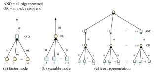
Considering a factor node with degree (i.e., there are UEs selecting the corresponding pilot), an edge connecting to this factor node can be recovered when the other edges connecting to this factor node have been recovered, as shown in Fig. 4(a). Similarly, as shown in Fig. 4(b), considering a variable node with degree (i.e., UE corresponding to this variable node sends sub-pilots to the BS), an edge connecting to a variable node with degree can be recovered when at least one of the other edges have been recovered. Let denote the probability that an edge connecting to a factor (variable) node with degree cannot be recovered. Then, we have
| (23) |
and
| (24) |
By averaging and over the edge distributions, the evolution of the average erasure probability during the iteration where is the maximum number of iterations, can be written as
| (25) |
The update process of and is shown in Fig. 4(c). Specifically, given initial values and , and can be derived by (25).
IV-A2 computation
The number of successful UEs obtained by the CICA algorithm can be written as
| (28) |
where denotes the probability that the CSI of one UE can be obtained successfully.
Based on the procedure of the CICA algorithm described in Subsection III-B, we can see that, the CICA algorithm first obtains the decoded uplink message via (14), and then obtains UE’s CSI via (15). Thus, if the uplink message of one UE can be decoded successfully, the CSI of this UE can be recovered successfully. Then, can be computed by
| (29) |
where is the bit error rate (BER) of the proposed CICA algorithm, which is larger than that using maximum likelihood (ML) decoding method [24], and can be written as
| (30) |
where step (a) follows from the fact that is a central chi-squared distribution with degree of freedom and that , and is the gamma function with parameter which is given by
| (31) |
IV-B Missed detection probability analysis
The missed detection probability refers to the ratio of the number of undetected active UEs to the total number of active UEs, which can be calculated as
| (35) |
IV-C Uplink throughput analysis
We define the uplink throughput as follows
| (37) |
where denotes the number of successful UEs where subscript “SchemeName” stands for the name of the scheme, denotes the overhead of the random access scheme, and is the frame length. Fig. 1 indicates that the amount of total overhead of the proposed GCICA-RA scheme is .
V Numerical Results
In this section, we first present the performance of the proposed GCICA-RA scheme, including the successful access probability, missed detection probability, and MSE performance of the CSI estimation method. Then, we make a comparison between the proposed GCICA-RA scheme, multiple-preamble grant-free RA scheme proposed in [20] and the traditional random access scheme in terms of the uplink throughput. For the traditional random access scheme, active UEs sends their randomly selected pilots along with their uplink messages to the BS, and the BS can only decode the uplink message of UE free from pilot collision.
In the simulation, we consider the urban micro scenario, where the path loss exponent is 3.8 [25]. The radius of the cell is 200 meters and all UEs are uniformly distributed among the location farther than 25 meters from the BS. Simulation parameters are shown in Table II. In addition, we utilize a LDPC code with 1/2 rate to code the payload data, and then employ the BPSK scheme to module the coded payload data. In the simulation, since the length of payload data is a few hundred bytes in M2M communications [26], the payload data size is set to 128 bytes to meet the communication requirements of M2M communications, and further to verify the proposed GCICA-RA scheme.
| Parameter | Value | ||
| (Code rate) | 1/2 | ||
|
2048 | ||
| (The number of antennas) | 400 | ||
|
5, 10, 15, 20 dB | ||
| (The number of pilots during each sub-pilot phase) | 6,9,10 | ||
| (The number of sub-pilot phases) | 2,3 | ||
| (The number of ICA classifiers) | 530 | ||
|
10 40 |


Fig. 5 shows how the successful access probability changes with the number of ICA classifiers , where dB, , , and . The upper bound for the successful access probability can be obtained according to (34). We can see from Fig. 5 that, with the increase of , the successful access probability increases dramatically first and then increases at a slower pace for different . The reason is that, the more the number of ICA classifiers, the more signals of one UE we can obtain, which further improves the decoding performance. We can also observe that, with the increase of , the successful access probability increases, and is close to the upper bound.
Fig. 6 shows how the missed detection probability changes with the number of ICA classifiers , where dB, , , and . The lower bound for the missed detection probability can be obtained according to (36). Fig. 6 illustrates that, with the increase of , the missed detection probability decreases dramatically first and then decreases at a slower pace for different . We can also note that, with the increase of , the missed detection probability takes small values and decreases, and is close to the lower bound.
Fig. 7 illustrates MSE performance of the proposed GCICA-RA, where dB, , , and . We can see from Fig. 7 that, with the increase of , MSE decreases dramatically first and then decreases at a slower pace for different . We can also note that MSE takes small values and decreases with the increase of .
Fig. 8 compares the uplink throughput between the proposed GCICA-RA, multiple-preamble grant-free RA schemes in [20], and the traditional random access scheme with different . We set , dB and . To see how the uplink throughput changes with the number of sub-pilot phases, we fix the length of the super pilot to 18, i.e., , and set to 2 and 3. To compare fairly, we ensure all random access scheme have the same pilot length and the same symbol length of the modulated uplink message. The upper bound for the uplink throughput of the proposed GCICA-RA is obtained via (38). Note that, since upper bounds for the uplink throughput of the proposed GCICA-RA are same for cases of and based on (38), we not distinguish these two upper bounds in this figure. It is observed that, the uplink throughput of is slightly higher than that of for the proposed GCICA-RA scheme. The reason is that the number of iterations of the SIC for is larger than that for on average, which results in the higher CSI estimation error [14] and further increase the equivalent noise introduced by the SIC algorithm. We also see that, the uplink throughput of the proposed GCICA-RA scheme is close to the upper bound, and significantly higher than those of baselines. With the increase of the number of active UEs, the gap between the uplink throughput of the proposed GCICA-RA scheme and those of baselines increases. This means that our proposed GCICA-RA is more suitable to crowded scenarios.
VI Conclusion
An GCICA-RA grant-free scheme was proposed to support massive connectivity for M2M communications in massive MIMO systems. The GCICA-RA scheme allows each active UE to transmit their super pilots and modulated uplink messages to the BS. Based on the received pilot signal and modulated uplink message, the BS utilizes a proposed GCICA algorithm to estimate the CSI and decode the uplink message of each active UE jointly, and then employs the estimated CSIs to detect active UEs. Simulation results demonstrated that, our proposed GCICA-RA scheme achieves performance gain even in the very crowded scenarios.
References
- [1] J. A. Stankovic, “Research directions for the internet of things,” IEEE Internet of Things Journal, vol. 1, no. 1, pp. 3–9, Feb. 2014.
- [2] P. Schulz, M. Matthe, H. Klessig, M. Simsek, G. Fettweis, J. Ansari, S. A. Ashraf, B. Almeroth, J. Voigt, I. Riedel, A. Puschmann, A. Mitschele-Thiel, M. Muller, T. Elste, and M. Windisch, “Latency critical IoT applications in 5G: Perspective on the design of radio interface and network architecture,” IEEE Communications Magazine, vol. 55, no. 2, pp. 70–78, Feb. 2017.
- [3] K. Ashton, “That ’internet of things’ thing,” RFiD Journal, vol. 22, pp. 97–114, Jan. 2009.
- [4] G. Wu, S. Talwar, K. Johnsson, N. Himayat, and K. Johnson, “M2m: From mobile to embedded internet,” Communications Magazine, IEEE, vol. 49, pp. 36 – 43, May. 2011.
- [5] C. VNI, “Cisco visual networking index: Forecast and trends, 2017¨c2022,” White Paper, 2018.
- [6] H. Q. Ngo, E. G. Larsson, and T. L. Marzetta, “Energy and spectral efficiency of very large multiuser MIMO systems,” IEEE Transactions on Communications, vol. 61, no. 4, pp. 1436–1449, Apr. 2013.
- [7] C. Xu, Y. Hu, C. Liang, J. Ma, and L. Ping, “Massive MIMO, non-orthogonal multiple access and interleave division multiple access,” IEEE Access, vol. 5, pp. 14 728–14 748, 2017.
- [8] C. Anton and M. Dohler, Machine-to-machine (M2M) Communications Architecture, Performance and Applications. Elsevier, Jan. 2015.
- [9] J. Yuan, H. Shan, A. Huang, T. Q. S. Quek, and Y. Yao, “Massive machine-to-machine communications in cellular network: Distributed queueing random access meets MIMO,” IEEE Access, vol. 5, pp. 2981–2993, 2017.
- [10] L. Sanguinetti, A. A. D’Amico, M. Morelli, and M. Debbah, “Random access in uplink massive mimo systems: How to exploit asynchronicity and excess antennas,” in 2016 IEEE Global Communications Conference (GLOBECOM), Dec. 2016, pp. 1–5.
- [11] Z. Dawy, W. Saad, A. Ghosh, J. G. Andrews, and E. Yaacoub, “Toward massive machine type cellular communications,” IEEE Wireless Communications, vol. 24, no. 1, pp. 120–128, Feb. 2017.
- [12] J. H. Sørensen, E. de Carvalho, and P. Popovski, “Massive MIMO for crowd scenarios: A solution based on random access,” in IEEE Globecom Workshops, Dec. 2014, pp. 352–357.
- [13] E. Björnson, E. de Carvalho, J. H. Sørensen, E. G. Larsson, and P. Popovski, “A random access protocol for pilot allocation in crowded massive MIMO systems,” IEEE Transactions on Wireless Communications, vol. 16, no. 4, pp. 2220–2234, Apr. 2017.
- [14] H. Han, Y. Li, and X. Guo, “A graph-based random access protocol for crowded massive MIMO systems,” IEEE Transactions on Wireless Communications, vol. 16, no. 11, pp. 7348–7361, Nov. 2017.
- [15] H. Han, X. Guo, and Y. Li, “A high throughput pilot allocation for M2M communication in crowded massive MIMO systems,” IEEE Transactions on Vehicular Technology, vol. 66, no. 10, pp. 9572–9576, Oct. 2017.
- [16] H. Han, Y. Li, and X. Guo, “User identity-aided pilot access scheme for massive MIMO-IDMA system,” IEEE Transactions on Vehicular Technology, vol. 68, no. 6, pp. 6197–6201, Jun. 2019.
- [17] J. Ahn, B. Shim, and K. B. Lee, “Ep-based joint active user detection and channel estimation for massive machine-type communications,” IEEE Transactions on Communications, vol. 67, no. 7, pp. 5178–5189, Jul. 2019.
- [18] L. Liu and W. Yu, “Massive connectivity with massive MIMO-Part I: Device activity detection and channel estimation,” IEEE Transactions on Signal Processing, vol. 66, no. 11, pp. 2933–2946, Jun. 2018.
- [19] H. Han, Y. Li, W. Zhai, and L. Qian, “A grant-free random access scheme for M2M communication in massive MIMO systems,” IEEE Internet of Things Journal, vol. 7, no. 4, pp. 3602–3613, Apri. 2020.
- [20] H. Jiang, D. Qu, J. Ding, and T. Jiang, “Multiple preambles for high success rate of grant-free random access with massive MIMO,” IEEE Transactions on Wireless Communications, vol. 18, no. 10, pp. 4779–4789, Oct. 2019.
- [21] L. Shen, Y. Yao, and H. Wang, “ICA based semi-blind decoding method for a multicell multiuser massive MIMO uplink system in Rician/Rayleigh fading channels,” IEEE Transactions on Wireless Communications, vol. 16, no. 11, pp. 7501–7511, Nov. 2017.
- [22] J. Shen, J. Zhang, and K. B. Letaief, “Downlink user capacity of massive MIMO under pilot contamination,” IEEE Transactions on Wireless Communications, vol. 14, no. 6, pp. 3183–3193, Jun. 2015.
- [23] G. Liva, “Graph-based analysis and optimization of contention resolution diversity slotted aloha,” IEEE Transactions on Communications, vol. 59, no. 2, pp. 477–487, Feb. 2011.
- [24] G. P. John, Digital Communications. Columbus, OH, USA: McGraw-Hill, 2001.
- [25] M. Fallgren and B. Timus, “Spatial channel model for multiple input multiple output (MIMO) simulations (Release 13),” document TR 25.996, 3GPP, Tech. Rep., Dec. 2015.
- [26] H. Lee, “The seven charicteristics of M2M traffic: Observations and implications,” IEEE Transactions on Vehicular Technology, vol. 2, pp. 341–349, Dec. 2013.