A Gallery of Gaussian Periods

Gaussian periods, certain sums of roots of unity introduced by Gauss, have played a key role in several mathematical developments. For example, Gauss employed them in his work on constructibility of regular polygons by unmarked straightedge and compass, as well as in number theory. In the past few years, realizations of their role in the supercharacter theory of Diaconis and Isaacs have led in new directions [3].

The fast computations afforded by modern technology provide new insights into Gaussian periods by enabling us to study them at a scale that was until recently unfathomable. In particular, large-scale plots of Gaussian periods display striking visual properties that were previously unknown (see, e.g., Figure 1). The goals of this paper lie in the intersection of the mathematical and artistic aspects of Gaussian periods:

• •

  Introduce Gaussian periods, together with new illustrations representing some of their visual features.

• •

  Introduce a new app, created in 2020, that quickly produces illustrations of Gaussian periods and is appropriate as a tool for art, exploratory mathematical research, illustration at scale, and pedagogy.

• •

  Summarize how mathematics controls some features, including colorings unexplained in earlier work.

Before proceeding, we clarify what we mean by the term Gaussian period. Given a positive integer $n$, an integer $\omega$ coprime to $n$, and an integer $k$, we set

$\displaystyle\eta_{n,\omega,k}:=\sum_{j=0}^{d-1}e^{\frac{2\pi i\omega^{j}k}{n}},$

where $d$ is the multiplicative order of $\omega$ mod $n$; that is, $d$ is the smallest positive integer such that $\omega^{d}\equiv 1\,(\operatorname{mod}n)$. When $k$ is relatively prime to $n$, we say that $\eta_{n,\omega,k}$ is a Gaussian period of modulus $n$ and generator $\omega$. In this paper, by a slight abuse of notation that coincides with the conventions employed in [7, 4, 8], we still call $\eta_{n,\omega,k}$ a Gaussian period of modulus $n$ and generator $\omega$ even when $k$ is not coprime to $n$. As we explain later in this paper, $\eta_{n,\omega,k}$ is a positive integer multiple of the Gaussian period $\eta_{\frac{n}{\gcd(n,k)},\omega,k}$, which allows us to preserve certain key structures of interest.

Each of the images in this paper is a plot in the complex plane of

$\displaystyle\mathsf{G}(n,\omega):=\left\{\eta_{n,\omega,k}:k=1,2,\ldots,n\right\}\subset\mathbb{C}.$

Mathematical principles guarantee that $\mathsf{G}(n,\omega)$ exhibits certain basic symmetries. For large values of $n$ (which we refer to as large scale), however, plots of $\mathsf{G}(n,\omega)$ also exhibit striking patterns and intricacies whose aesthetic properties can be appreciated even by those without mathematical training.

That large-scale plots of Gaussian periods exhibit such variety and intricate patterns was a surprise. This was discovered by B. Lutz, an undergraduate, in the course of his senior thesis. In his explorations, he also introduced a coloring scheme, which is employed in the plots in this paper and discussed in the next section.

A new app, Gaussian Periods (written in Swift for Apple computers and freely available [6]) was produced in 2020 by the first named author, with assistance from R. Lipshitz. This app:

• •

  plots Gaussian periods faster than previous code (including the aforementioned Mathematica code), taking seconds to produce images that used to take hours;

• •

  allows larger scale plots than previously possible (e.g., Figure 4, which contains over 9 million points), which can be useful for exploring or illustrating asymptotic behavior;

• •

  does not require programming experience or mathematical expertise;

• •

  allows one to quickly modify values of $n$ and $\omega$, as well as a coloring parameter $c$; and

• •

  includes an option to save layers suitable for further steps, e.g., manipulation in Adobe Photoshop to customize color choices (as was done to produce the images in this paper).

As a result, the app is suitable for projects ranging from art to exploratory mathematical investigations to illustration. We also used it to produce all the images in this paper. To improve the image quality in this paper, we layered the different color components (plotting all the points corresponding to a color at the same time), which is assisted by the layers option in the app.

While notions of “beauty” and “aesthetic appeal” are subjective, symmetry has often appeared in discussions of beauty in both art and math, dating back to the ancient Babylonians. In a historical context, given the algebraic origins of Gaussian periods, it is fitting to note that symmetry originally became a prominent concept in mathematics not through geometry, but through algebra [9, Preface]. Gaussian periods, together with the various symmetries they exhibit, can also be considered of independent artistic merit and be appreciated in their own right (even by those with no mathematical training). More broadly, patterns in plots of certain other families of algebraic numbers have also been recognized for their beauty [1]. For those who wish to delve further into philosophical considerations of the artistic merits of Gaussian periods, a brief survey of visual aesthetics in similar mathematical contexts can be found in [2, pp. 121-4].

Whether focusing on art or math, a coloring scheme can be used to highlight some structures in $\mathsf{G}(n,\omega)$ for a given $n$ and $\omega$. Following [7, §3], fix a positive integer $c\mid n$ and, for $j=1,2,\ldots,c$, assign the same color to all points in the set $\{\eta_{n,\omega,k}:k\equiv j\,(\operatorname{mod}c)\}$. Two points $\eta_{n,\omega,k}$ and $\eta_{n,\omega,\ell}$ might have the same color even if $k\nequiv\ell\,(\operatorname{mod}c)$, since $\eta_{n,\omega,k}=\eta_{n,\omega,k\omega^{j}}$ for all integers $j$.

Since this is the coloring scheme employed in each of the images here (and is implemented in Gaussian Periods), we begin with small-scale examples to help readers grasp the subtleties of this coloring scheme.

This approach to coloring was chosen not as a way to illustrate a particular mathematical principle but rather as a recipe Lutz discovered that produced visually appealing pictures. In fact, in the final paragraph of [7], he and his coauthors note that this approach to coloring is ad hoc and that “a general theory is necessary to formalize our intuition.”

Through the lens of Galois theory (which was never considered in prior work on illustrating $\mathsf{G}(n,\omega)$), the above coloring scheme can be linked to mathematical structure. The main theorem of Galois theory gives a bijection between the subfields of $\mathbb{Q}\left(\zeta_{n}\right)$, with $\zeta_{n}$ a primitive $n$th of unity, and the subgroups of the Galois group $G:=\mathrm{Gal}\left(\mathbb{Q}\left(\zeta_{n}\right)/\mathbb{Q}\right)=\operatorname{Aut}\left(\mathbb{Q}\left(\zeta_{n}\right)\right)$, which is identified with $\left(\mathbb{Z}/n\mathbb{Z}\right)^{\times}$ via

	$\displaystyle\left(\mathbb{Z}/n\mathbb{Z}\right)^{\times}$	$\displaystyle\overset{\sim}{\rightarrow}G$
	$\displaystyle[m]$	$\displaystyle\mapsto\psi_{m}$
	$\displaystyle\psi_{m}\Big{(}\sum_{j}a_{j}\zeta_{n}^{j}\Big{)}$	$\displaystyle:=\sum_{j}a_{j}\left(\zeta_{n}^{m}\right)^{j},\hskip 36.135pta_{j}\in\mathbb{Q}.$

Each subgroup $H\subseteq G$ corresponds to the fixed field $\mathbb{Q}\left(\zeta_{n}\right)^{H}:=\left\{z\in\mathbb{Q}\left(\zeta_{n}\right):\psi(z)=z\mbox{ for all }\psi\in H\right\}$. Then $H$ is the Galois group of $\mathbb{Q}\left(\zeta_{n}\right)$ over $\mathbb{Q}\left(\zeta_{n}\right)^{H}$, i.e., the group of field automorphisms of $\mathbb{Q}\left(\zeta_{n}\right)$ fixing $\mathbb{Q}\left(\zeta_{n}\right)^{H}$, and $G/H$ is the Galois group of $\mathbb{Q}\left(\zeta_{n}\right)^{H}$ over $\mathbb{Q}$, i.e., the group of field automorphisms of $\mathbb{Q}\left(\zeta_{n}\right)^{H}$.

To help identify elements of the subfields of $\mathbb{Q}\left(\zeta_{n}\right)$, students in Galois theory courses are sometimes assigned to determine Gaussian periods (e.g., see [5, §14.5]). Indeed, if $H=\langle\omega\rangle$, then

$$\eta_{n,\omega,k}=\sum_{\psi\in H}{\left(\psi\left(\zeta_{n}\right)^{k}\right)}=\sum_{\psi\in H}\psi\big{(}\zeta_{n}^{k}\big{)}\in\mathbb{Q}\left(\zeta_{n}\right)^{H},$$

So the plot of $\mathsf{G}(n,\omega)$ contains a (rescaled) plot of $\mathsf{G}(\frac{n}{\gcd(n,k)},\omega)$. If $c$ is the coloring number, then the plot of $\mathsf{G}(n,\omega)$ contains a single-colored plot of $\mathsf{G}(\frac{n}{c},\omega)$, rescaled by a factor of $\frac{\mathrm{ord}_{n}(\omega)}{\mathrm{ord}_{n/c}(\omega)}$, with $\mathrm{ord}_{m}(\omega)$ denoting the multiplicative order of $\omega\,(\operatorname{mod}m)$. For clarification, we illustrate this in a simple example.

Regarding the current coloring scheme, if two elements of $\mathbb{Z}/n\mathbb{Z}^{\times}\cong\mathrm{Gal}(\mathbb{Q}(\zeta_{n})/\mathbb{Q})$ are congruent $\mod c$, then the corresponding elements of the Galois group restrict to the same element of $\mathrm{Gal}(\mathbb{Q}(\zeta_{c})/\mathbb{Q})$. So, for example, given an element $\psi\in\mathrm{Gal}(\mathbb{Q}(\zeta_{c})/\mathbb{Q})$ and an integer $a$, all points $\Psi(\eta_{n,\omega,a})$, as $\Psi$ ranges over the extensions of $\psi$ to $\mathbb{Q}(\zeta_{n}),$ are colored the same. There are also other natural coloring schemes. For example, an option (called “period squared”) in Gaussian Periods is to color $\eta_{n,\omega,k}$ and $\eta_{n,\omega,-k}$ the same, thus creating symmetry across the real axis. This corresponds to coloring the points in the Galois orbit of the complex conjugation automorphism the same. More generally, one might color all points in some other given Galois orbits the same. Furthermore, our reformulation in terms of elements of fixed fields should naturally generalize beyond Gaussian periods to the illustration of symmetries in other settings beyond the scope of this short paper (such as finite nonabelian extensions of $\mathbb{Q}$).

Symmetry is the most obvious feature in typical Gaussian-period plots. We say that $\mathsf{G}(n,\omega)$ has $k$-fold dihedral symmetry if $\mathsf{G}(n,\omega)$ is invariant under the action of the dihedral group of order $2k$. That is, $\mathsf{G}(n,\omega)$ is invariant under complex conjugation and rotation by $2\pi/k$ about the origin. It turns out that $\mathsf{G}(n,\omega)$ has at least $\gcd(\omega-1,n)$-fold dihedral symmetry [4, Prop. 3.1]. This symmetry refers to the uncolored graph; the colors highlight additional features beyond the initial symmetry. This is illustrated in Figure 3.

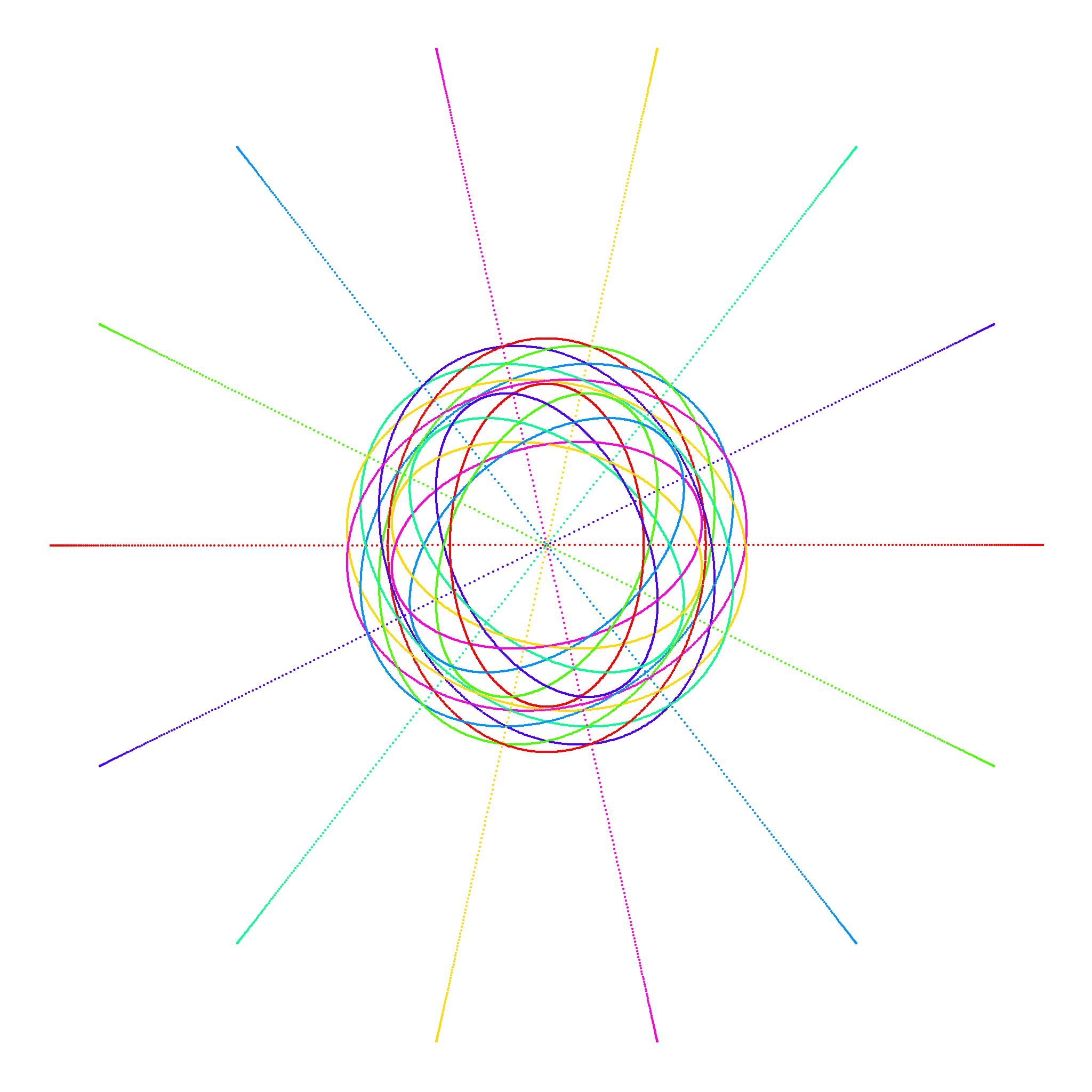
Gaussian period plots often demonstrate great structural coherence if the parameters $n$ and $\omega$ vary in the appropriate manner. The following “filling out” of various shapes was discovered in [4, Thm. 6.3]. See the thorough exposition in [7, Thm. 1]. Let $q=p^{a}$ be a nonzero power of an odd prime and let $\omega=\omega(q)$ be such that $d=|\langle\omega\rangle|$ divides $p-1$. Then $\mathsf{G}(q,\omega)$ is contained in the image of the Laurent polynomial function $g:\mathbb{T}^{\varphi(d)}\to\mathbb{C}$ defined by

$$g(z_{1},z_{2},\ldots,z_{\varphi(d)})=\sum_{k=0}^{d-1}\prod_{j=0}^{\varphi(d)-1}z_{j+1}^{b_{k,j}},$$

where the integers $b_{k,j}$ are determined by $t^{k}\equiv\sum_{j=0}^{\varphi(d)-1}b_{k,j}t^{j}\,(\operatorname{mod}\Phi_{d}(t)).$ Here $\mathbb{T}$ denotes the unit circle in $\mathbb{C}$, $\varphi$ is the Euler totient function, and $\Phi_{d}$ denotes the $d$th cyclotomic polynomial. For a fixed $d$, as $q$ becomes large, $\mathsf{G}(q,\omega)$ “fills out” the image of $g$; see Figure 4.

With ellipses, hypocycloids, and so forth as primitive graphical elements, one can use the Chinese remainder theorem to produce new images of startling complexity (as explained in [8]). We content ourselves here with a few aesthetically pleasing images produced in such a manner; see Figure 5. We encourage the reader to enjoy more examples by experimenting with our app Gaussian Periods (freely available at http://www.elleneischen.com/gaussianperiods.html).

Ellen Eischen was partially funded by NSF grant DMS-1751281. Stephan Ramon Garcia was partially funded by NSF grant DMS-1800123. This material is based partly upon work supported by the NSF grant DMS-1439786 and the Alfred P. Sloan Foundation award G-2019-11406 while the authors were in residence at the Institute for Computational and Experimental Research in Mathematics (ICERM) in Providence, RI, during the Illustrating Mathematics program (Fall 2019). We thank R. Lipshitz for help with the code.

References

- [1] J. Baez. The beauty of roots. 2011. http://math.ucr.edu/home/baez/roots/.
- [2] T. M. Brown, “Kaleidoscopes, Chessboards, and Symmetry,” Journal of Humanistic Mathematics, vol. 6, no. 1, 2016, pp. 110–126. https://scholarship.claremont.edu/jhm/vol6/iss1/8
- [3] J. L. Brumbaugh, M. Bulkow, P. S. Fleming, L. A. G. German, S. R. Garcia, G. Karaali, M. Michal, A. P. Turner, and H. Suh. “Supercharacters, exponential sums, and the uncertainty principle.” Journal of Number Theory, vol. 144, 2014, pp. 151–175.
- [4] W. Duke, S. R. Garcia, and B. Lutz. “The graphic nature of Gaussian periods.” Proceedings of the American Mathematical Society, vol. 143, no. 5, 2015, pp. 1849–1863.
- [5] D. S. Dummit and R. M. Foote. Abstract Algebra, 3rd ed., John Wiley & Sons, 2004.
- [6] E. E. Eischen and R. Lipshitz. Gaussian Periods. http://www.elleneischen.com/gaussianperiods.html, 2020.
- [7] S. R. Garcia, T. Hyde, and B. Lutz. “Gauss’s hidden menagerie: from cyclotomy to supercharacters.” Notices of the American Mathematical Society, vol. 62, no. 8, 2015, pp. 878–888.
- [8] B. Lutz. “Graphical cyclic supercharacters for composite moduli.” Proceedings of the American Mathematical Society, vol. 147, no. 9, 2019, pp. 3649–3663.
- [9] I. Stewart. Why Beauty is Truth: The History of Symmetry. Basic Books, 2007.