A functional regression model for heterogeneous BioGeoChemical Argo data in the Southern Ocean
Abstract
Leveraging available measurements of our environment can help us understand complex processes. One example is Argo Biogeochemical data, which aims to collect measurements of oxygen, nitrate, pH, and other variables at varying depths in the ocean. We focus on the oxygen data in the Southern Ocean, which has implications for ocean biology and the Earth’s carbon cycle. Systematic monitoring of such data has only recently begun to be established, and the data is sparse. In contrast, Argo measurements of temperature and salinity are much more abundant. In this work, we introduce and estimate a functional regression model describing dependence in oxygen, temperature, and salinity data at all depths covered by the Argo data simultaneously. Our model elucidates important aspects of the joint distribution of temperature, salinity, and oxygen. Due to fronts that establish distinct spatial zones in the Southern Ocean, we augment this functional regression model with a mixture component. By modelling spatial dependence in the mixture component and in the data itself, we provide predictions onto a grid and improve location estimates of fronts. Our approach is scalable to the size of the Argo data, and we demonstrate its success in cross-validation and a comprehensive interpretation of the model.
Keywords: clustering, functional regression, penalized splines, physical and biogeochemical oceanography, spatially-dependent data
1 Introduction
The rapid growth of high-resolution data motivates continued advances in flexible and efficient statistical methodology. One prime example is the Argo data, which is collected by autonomous devices drifting through the world oceans called floats that measure temperature and salinity. Argo floats collect their data in so-called profiles, collections of measurements at various depths for fixed points in time and space (see Figure 1 and Argo, 2020). The Argo data has greatly enhanced our understanding of the physical nature of the upper 2000 meters of the oceans with near-uniform spatial sampling of these variables (Johnson et al., 2022). Argo floats determine their own depth through pressure measurements as an increase in 1 decibar in pressure occurs for each additional meter of depth (approximately). From here on, we will thus often use pressure rather than depth to refer to a float’s vertical position in the ocean.
An important expansion of the Argo Project’s goals is Biogeochemical (BGC) Argo, which has added a limited number of floats that also measure oxygen and nitrate, among other variables. We focus on Argo data in the Southern Ocean because the majority of the BGC Argo data has been collected under the Southern Ocean Carbon and Climate Observations and Modeling (SOCCOM) project (Riser et al., 2023, soccom.princeton.edu). The increased availability of biogeochemical data is important to improve our understanding of vital biogeochemical processes such as the biological carbon pump and air-sea CO2 exchanges, monitor changes such as ocean deoxygenation and acidification, and improve estimates of the carbon budget (Bittig et al., 2019; Claustre et al., 2020; Gray et al., 2018). However, BGC floats use additional sensors, leading to higher fixed and maintenance costs than Core Argo floats (that is, those that measure only temperature and salinity). Thus, it is not practical to introduce the same coverage as achieved by Core Argo floats. Indeed, in the Southern Ocean during 2020, Core Argo floats collected approximately 12000 profiles while BGC Argo floats collected just 3600 over the same time period (see Figure 1).


When modelling biogeochemical data, it is thus desirable to utilize the more prevalently available Core Argo data in addition to the available BGC data to improve prediction and estimates and reduce uncertainty. This paper is aimed towards this goal, and our main contributions are as follows.
-
1.
We develop a descriptive statistical model on the joint distribution of oxygen, temperature, and salinity in the Southern Ocean. The model fully takes into account the functional nature and space-time information of the Argo data.
-
2.
Based on this model, and leveraging the more readily available temperature and salinity data, we address methodological and computational issues related to the functional prediction and interpolation of oxygen levels at arbitrary locations.
While both (a) and (b) are of significant scientific as well as statistical interests, we are unaware of any existing work that considers them comprehensively. Below, we explain our approaches in more detail.
The basic building block for our model is a spatio-temporal, function-on-function regression model that encodes the functional relationship between the temperature, salinity and oxygen profiles across all pressure levels ranging from to decibars. This enables us to predict oxygen profiles using temperature and salinity profiles. It also facilitates the estimation and prediction of other quantities of scientific interests such as derivatives and integrals of the profiles (Park et al., 2023).
One major challenge of modelling Argo data in the Southern Ocean is that the transition from warmer subtropical waters in the north to colder Antarctic waters does not occur smoothly. Instead, ocean properties in that region are characterized by a series of sudden changes, occurring at so-called fronts — sharp transition zones generally aligned east–west (Chapman et al., 2020; Orsi et al., 1995). In particular, the contrasting behavior of oxygen in various regimes of the Southern Ocean has been well established in Bushinsky et al. (2017). Consequently, any stationarity assumption on the data across different fronts would be violated. However, it is established that ocean properties in any region between fronts tend to be homogeneous (Chapman et al., 2020). To address this challenge, we augment our functional regression model with a latent mixture component aimed at capturing regional information. Our model thus describes aspects of the joint distribution of oxygen, temperature, and salinity modulated by different regimes in the Southern Ocean. In our analyses, we demonstrate that the dependence structure in pressure of these three variables varies critically across the regimes estimated through the mixture model. As a byproduct we obtain estimates for the locations of ocean fronts and how they vary with time. These are of considerable scientific interest in their own right and have been the subject of research in the oceanographic literature (Chapman et al., 2020). Consequently, they constitute an additional key contribution of this work.
Identifying ocean fronts through the use of clustering and mixture models in oceanography has recently gained significant traction. For example, Jones et al. (2023, 2019) focus on the Southern Ocean region; Rosso et al. (2020), Boehme and Rosso (2021), and Fonvieille et al. (2023) consider subregions of the Southern Ocean, while Maze et al. (2017), Poropat et al. (2023), and Houghton and Wilson (2020) analyze other oceanographic areas. Most of these works use standard Gaussian mixture models. The primary difference between this literature and our work here is that we account for the spatio-temporal dependence for the cluster memberships and the data within each cluster while these critical aspects are ignored in the above cited works. We accomplish this by encoding the spatio-temporal dependence of cluster memberships using a Markov random field model (Liang et al., 2020; Jiang and Serban, 2012; Besag, 1975). In particular, this enables predictions at any location whether temperature and salinity data are available or not. An important application of this is mapping, or the creation of gridded products, where data sampled at irregular locations in space and time are used to provide estimates at a standard grid (for example, Roemmich and Gilson, 2009; Gray and Riser, 2014).
When temperature and salinity measurements are available, predictions of oxygen may be straightforwardly made using off-the-shelf methodology. A well-known example in that regard is the random forest approach of Giglio et al. (2018), which produces highly accurate predictions of oxygen at fixed pressure levels using temperature and salinity data. For this scenario, we provide comparisons of our mode-based approach with the random forest approach of Giglio et al. (2018). However, when estimating the oxygen level at a location or a pressure level where temperature and/or salinity information is not available, the random forest approach requires an additional step of interpolating predicted oxygen data onto this location. Our model-based approach, on the other hand, readily provides direct predictions as well as estimated uncertainty of oxygen levels at arbitrary locations and pressure levels using nearby temperature and salinity data without interpolations.
Our approach also involves advancements in both statistical methodology and implementation. There is a rich literature on function-on-function regression, including the seminal paper Yao et al. (2005) and Zhou et al. (2008), while modelling spatio-temporal dependence in univariate functional data has been studied extensively by, e.g., Zhou et al. (2010); Jiang and Serban (2012); Liang et al. (2020). However, we are unaware of any development of function-on-function regression models that accounts for spatio-temporal correlation in the functional response and predictor variables. Furthermore, to the best of our knowledge, functional kriging and cokriging problems in the context of functional mixture models have not been explored at all. The SOCCOM Argo data considered here alone consists of more than fifteen thousand locations and millions of observations. Consequently, reducing the runtime and memory usage of the model estimation and prediction procedure is essential. This work is accompanied by an R package implementing our methodology where crucial parts of the estimation and prediction procedure are written in C++.
We finally briefly describe the organization of the rest of the paper. In Section 2, we propose a novel mixture model for multivariate, functional data with spatial dependence. In Section 3, we discuss parameter estimation, prediction, and model selection. In Section 4, we describe our analysis on the Argo data, including the description of the estimated model, evaluation of oceanographic front estimates, and cross-validation experiments. Finally, we discuss limitations and potential improvements to our work in Section 5.
2 The Data and the Model
Argo data is publicly available from the Argo Global Data Assembly (GDAC, Argo, 2020) after it undergoes various data control measures (Maurer et al., 2021). A precise description of the data under consideration is given in the supplement Section S1.
Notationally, our data consists of profiles at locations in the Southern Ocean and corresponding points in time . We use to denote the spatial domain and use the positive real axis as time domain. To simplify notation, we will denote a space-time coordinate by . At each point , we observe profiles of a biogeochemical quantity (oxygen) as well as temperature and salinity each at pressure levels . Consequently, oxygen data for one profile for is then and for temperature and salinity and . Even though the number of observations as well as the pressure indexes may vary between temperature, salinity and oxygen, we suppress this in our notation for clarity of presentation. Motivated by this structure in the data, we model the observations as point evaluations from unknown random functions of pressure, observed with additive measurement errors:
We use calligraphic letters to denote the underlying functions and regular letters for the observations. For each index , we model the functions and as elements of a Hilbert space which we choose to be , the Hilbert space of square integrable functions on the closed interval because most Argo profiles consist of measurements between 0 and 2000 decibars. In addition, we assume sufficient regularity of the functions to ensure pointwise evaluations, and we later impose a smoothness penalty on the 2nd derivative. The measurement errors , and are assumed to be i.i.d. Gaussian random variables with zero mean and variances and to be estimated from the data. The main focus of our model is the biogeochemical quantity , so we collect temperature and salinity in a covariate vector of functions . Combined, this yields two space-time, function-valued random fields and .
Modelling Ocean Fronts via a Latent Mixture Component As stated in the introduction, one main challenge with the Argo data is its nonstationary. To account for this, much of the previous work on the Argo data uses local approaches for example via sliding windows; see for example, Kuusela and Stein (2018); Yarger et al. (2022); Park et al. (2023). A locally-stationary model is estimated for each window, and since parameters are estimated anew for each window, the model adapts to varying covariance structures in different locations. However, in the Southern Ocean, this approach may not be suitable due to the sharp and sudden changes in water properties at the ocean fronts. Moreover, due to the circumpolar nature of the ocean fronts, water properties may stay homogeneous across long distances which any local approach will fail to fully utilize. In order to explicitly model the ocean fronts, we partition the data into clusters, with ocean fronts representing the boundaries between clusters. We use a latent field where each is a random variable taking value in for some to be specified. We then model
where the random fields and govern the spatio-temporal covariance structure in cluster . Here is the usual indicator function.
For , we employ a commonly used Markov random field model (cf. Jiang and Serban, 2012; Liang et al., 2020), where the marginal distribution given appropriately defined neighbors is given by
| (1) |
We use -nearest neighbor graphs to define the neighborhood structure based on the distance to account for the anisotropy in the Argo data. The additional weighting by the inverse distance follows the intuition that profiles that are close should provide better cluster information than profiles that are further away. This also reduces the importance of the choice of the number of nearest neighbors to construct the underlying graph which we chose to be 15. Consequently, we found that reasonably varying this number has negigible impact. The Markov random field model allows cluster memberships to be interpolated between the irregularly-sampled profile locations. Moreover the Markov structure yields computational advantages by using a pseudo-likelihood approximation as in Besag (1975).
We found that incorporating a temporal component in the distance is important. Indeed, we implemented a Markov random field that used only space (without a seasonal component) and found that in many locations this gave conflicting information on cluster membership from winter versus summer profiles.
Spatio-Temporal Function on Function Regression Within each cluster, we use the following spatial regression model to specify the joint distribution of and :
| (2) |
where the are linear operators and the are functional, spatio-temporally correlated residuals that are independent of . Here, and are mean functions of pressure for the response and predictors, respectively, in the -th group and depend on time . In the mean function , we include seasonality using a Fourier basis as in Roemmich and Gilson (2009):
The evaluation then represents the average (across the year) mean of oxygen for group at pressure , while the for describe seasonal variations in that mean based on sines and cosines. We take in this case to capture the main seasonality component, which is half of the number basis functions used in Roemmich and Gilson (2009) because in Antarctica there are only two seasons (NASA, 2024). The mean functions of the predictors have identical form. Next, we employ a Karhunen-Loève type expansion along the pressure dimension,
| (3) |
in order to model the spatio-temporal correlation structure through the principal component random fields and (Zhou et al., 2010). The functions and form an orthonormal basis for and respectively for each and are called the principal component functions (PCFs). In practice, the infinite sums have to be truncated appropriately. Through the joint principal component decomposition of , dependence between predictors (temperature and salinity) is modeled. Quantifying this dependence in the model is critical, since these variables are known to be dependent. For example, temperature, salinity, and pressure jointly determine potential density which is known to be generally monotone as a function of pressure (Section 3.5 of Talley, 2011). The coefficient random fields and are assumed to be independent across cluster and component . Using (3) in (2), and afterwards truncating the infinite sums after and terms, we obtain
We model the random fields constituting the principal component scores as Gaussian random fields as is common in spatial statistics. Because they have zero mean, it remains to specify their covariance structure. A popular choice is the Matérn covariance function as advocated for by Stein (2013). However, for the Argo data an isotropic covariance function such as the standard Matérn covariance is likely not appropriate. For example, Kuusela and Stein (2018) found that, typically, the correlation range scales are different for longitude and latitude. We follow Guinness (2021) who, when modelling Argo data, used spatial deformation of the sphere via gradients of the spherical harmonics to model anisotropies. Concretely, we deform the sphere by mapping a point where is the weighted sum of gradients of the spherical harmonics of degree 2 at . The weights will be learned from the data. We then use the following covariance
| (4) |
where , is the modified Bessel function of the second type and for ,
where is the standard Euclidean norm (chordal distance). An R implementation of this covariance function is readily available in the GpGp package (Guinness et al., 2021). Generally, we found that allowing more flexibility in the covariance function improved prediction performance. The smoothness parameter , variance parameter , and range parameter and govern properties of the Matérn model for the -th predictor principal component of the -th group. We use the same covariance form for .
3 Model Estimation and Prediction
The mean functions, the PCFs, and the functions are unknown and have to be estimated from the data. To do so, we use a cubic B-spline basis, a common choice in functional data analysis with favourable computational and provable optimality properties (Wahba, 1990; Hsing and Eubank, 2015). Specifically, if are the elements of the cubic B-spline basis on [0, 2000] write . Then we use
where is the -th column of the matrix of spline coefficients for the seasonal means of and is the corresponding matrix for the covariates, is the -th column of the matrix containing the coefficients for the PCFs for , and the matrix contains the coefficients for the . Similarly, is a matrix. For the PCFs, we impose the following constraints to enforce orthonormality:
| (5) |
Here is the standard Kronecker product and is the identity matrix. For identifiability reasons, we require the first entries in each column of and to be positive and order the PCFs by the marginal variances of the random fields constituting the principal component scores.
Remark 1
A common approach to enforce the orthogonality constraints in (5) is to use an orthogonalized spline basis and then require and ; see Zhou et al. (2010) and Liang et al. (2020), among others. However, for datasets as large as the Argo data, this becomes impractical because the evaluation matrices (at observed data points) for orthogonalized splines are less sparse compared to regular B-splines. We outline in the supplement Section S9 that regular B-splines can be used to obtain orthonormal principal components with a proper orthonormalization step.
3.1 Monte Carlo EM Algorithm
Notationally, we collect all observations in the vector and all temperature and salinity observations in the vector . Data from a single profile will be denoted by and respectively. The corresponding latent principal component scores and the cluster memberships are collected in the vectors , and respectively. We collect the spline coefficient matrices, the covariance parameters, and the MRF parameter in the set . To fit the model, we aim to maximize the penalized log-likelihood of the observed data
| (6) |
where denotes a roughness penalty and denotes the likelihood function. Corresponding to our choice of cubic B-splines, we use integrated squared second derivatives of the respective functions as penalty (cf. Theorem 6.6.9; Hsing and Eubank, 2015).
Because the random vectors and are unobserved, direct maximization of (6) is not feasible. A useful tool for such scenarios is the EM algorithm (Dempster et al., 1977). It consists of initializing the parameters to and alternating between the following two steps for until convergence:
-
1.
E-step: Compute .
-
2.
M-step: Update the parameters via .
Direct application in of the EM algorithm in our case is not possible because is not tractable. Instead, we use a Monte Carlo EM algorithm (Wei and Tanner, 1990).
Monte Carlo E-Step. We use importance sampling to estimate . That is, we fix and create samples for from a proposal distribution and approximate via
| (7) | ||||
where the quantities are called the importance sampling weights and are the self-normalized weights. For details on importance sampling, see Robert and Casella (2004). In a similar situation, Liang et al. (2020) use a Markov Chain Monte Carlo EM algorithm by employing a Gibbs sampler to generate samples of the latent random variables. When we applied their sampler to the Argo data, we found that the resulting Markov Chain mixes slowly and thus obtained suboptimal results. Both Monte Carlo approaches are motivated by the fact that, due to the dependence in the data and the discrete nature of the cluster memberships, the conditional distribution is not tractable in closed form. A brief discussion and comparison as well as details on our proposal can be found in the supplement Section S4.
M-step. To update the parameters set . The log-likelihood of the complete data factors into separate terms
allowing for most parameters to be updated separately. A closed form solution exists for most of the parameters, except for the spatial parameters and the MRF parameter for which numerical maximization is necessary. The updating formulas are given in the supplement Section S8. For EM algorithms, initialization can play an important role. We provide a detailed initialization procedure that we found to work well in the supplement Section S10.
3.2 Model Selection
We choose the number of clusters by domain knowledge (see e.g. Chapman et al., 2020) as indicated in the introduction and have already specified our MRF structure. It remains to choose the number of principal components and the smoothing penalties. The number of knots for the spline basis plays a small role in model fit as long as there are sufficiently many to approximate relevant functions because we impose a smoothing penalty (cf. Zhou et al., 2008). For the remaining tuning parameters, we use an AIC criterion where we use again importance sampling to approximate the intractable observed data likelihood. Let denote the model degrees of freedom, samples of the latent field from a proposal and the corresponding weights. Then our AIC criterion is
| (8) |
The proposal is slightly different from the one used during the EM-algorithm; details are found in the supplement Section S4. To determine , we take into account the smoothing penalty imposed on functions as in Wei and Zhou (2010). We choose different smoothing parameters for , , , , and ; for simplicity, we assume that these parameters do not vary over the cluster or principal component index.
A frequently used alternative choice is to use the output of the Monte-Carlo E-step from the last EM-iteration as an approximation to the true likelihood (Huang et al., 2014; Liang et al., 2020). This did not work well for the Argo data as anticipated by Ibrahim et al. (2008), and we found that the cost of one additional E-step of (8) was offset by a more reliable model selection.
3.3 Prediction
To provide functional predictions at new locations using the observed data and we use the conditional expectation . In this setting, we may include additional data (for example, temperature and salinity data at or nearby ) in not included in model training. Furthermore, we stress that one does not need temperature and salinity at to construct predictions at these locations. Similar to the E-step, closed-form expressions of the conditional expectation are not available due to the latent field . Therefore, we again use importance sampling. Concretely, we generate samples of the latent field (which now includes the new locations ) from the Potts model (1) and then set
| (9) |
where are the importance weights. The conditional (co)variances for oxygen at varying pressures or locations are formed using the importance samples and the law of total (co)variance. For example, for one location and pressure , we compute:
| (10) | ||||
Due to the Gaussianity of the latent fields and , closed from expressions for the quantities appearing in (9) and (10) are available, see the supplement Section S5. Inference for the latent field at new locations is based on the samples .
Modeling functional dependence enables us to construct confidence bands for for a location such that we expect to lie entirely (for all ) within the band. We construct bands based on the estimates of and using the approach of Choi and Reimherr (2018). When we predict that belongs to a certain cluster with probability very close to 1, these bands may be directly applied; otherwise, bands from different groups should be considered individually. Our functional approach also yields principled predictions for linear functionals such integrals and derivatives of that are frequently of interest for Argo data.
3.4 Computational Details
Due to the size of the Argo data considered here – alone the SOCCOM data consists of more than fifteen thousand locations and millions of observations – naive implementation of the above EM-algorithm is computationally expensive. The most computationally demanding steps are the covariance parameter estimation of the latent random fields and during the M-step as well as computing their conditional distribution for the E-step and for predictions. The main tool we employ for these steps is Vecchia’s approximation Katzfuss et al. (2020) but additional steps are necessary. We outline them in the supplement Section S7.
4 Data Analysis Results
Here, we present results from our analysis of the Argo data, beginning with the estimated model in Section 4.1. We then provide a cross-validation study to assess prediction performance in Section 4.2 and present our data product of comprehensive functional predictions in Section 4.3.
4.1 Description of estimated model
Our final model uses 18 principal components for the response and 18 for the predictors even though our AIC criterion (provided in the supplement Section S2) indicates that even more principal components could be used. However, we found that additional principal components did not improve prediction performance and increased computation time.


In Figure 2, we plot the predicted clusters for four months of the year. Our clusters are ordered by their mean temperature function’s value at 1000 decibars. We also plot in black lines previous estimates of fronts using the same criteria as Bushinsky et al. (2017) based on the 2004-2018 Roemmich and Gilson (2009) estimate, see also Orsi et al. (1995). These can be described as follows. South of the southern-most line is the Seasonal Ice Zone, whose northern boundary is defined by the maximum extent of sea ice. The next zone is defined by the maximum extent of sea ice in the south and the Subantarctic front in the north, which contains the Antarctic Circumpolar Current (ACC), a strong ocean current that encircles Antarctica (Bushinsky et al., 2016). The final plotted front is the Subtropical front. These traditional estimates of fronts are generally represented well by our clustering plotted in Figure 2. For example, our first cluster matches the Seasonal Ice Zone for most months. Clusters 2 and 3 make up the main component of the ACC, with their northern boundary generally aligning with the Subantarctic front. Clusters 4 and 5 define waters above the Subantarctic front, with cluster 4 more concentrated in the Pacific and Atlantic. There are also substantial seasonal variations, underscoring the importance of modeling the contrast between winter and summer in the Southern Ocean. For example, in the austral winter (July) clusters 2 and 4 are disproportionately represented while cluster 5 is nearly absent. Between cluster boundaries, the predicted cluster has relatively high probability, while there is some uncertainty on their boundaries. In the supplement Section S3, we also compare with Jones et al. (2019)’s analysis of 6 clusters from temperature data.
In general, the clusters are influenced by a variety of processes occurring in the Southern Ocean. Near the ocean surface, interactions with the atmosphere result in higher levels of oxygen dissolved near oxygen’s saturation point in water. In this level, the primary determinant of dissolved oxygen is the water’s capacity to hold oxygen, which increases as temperature or salinity decreases (see Section 4.5 of Talley, 2011). Oxygen is generally decreasing for a water mass as a function of “age,” that is, the time since it has interacted with the atmosphere (Section 3.6 of Talley, 2011), due to the utilization of oxygen by ocean life. In the Southern Ocean, upwelling (water at lower depths rising to the surface) of older, low-oxygen water occurs near around the Southern ACC front (approximately, our cluster 2), after which it splits both poleward and toward the equator at the surface (Gray et al., 2018). During the winter, ice cover blocks the potential uptake of oxygen to the upper layer of the ocean in the Seasonal Ice Zone; freezing water also ejects its salinity as it freezes, increasing the salinity of the surrounding water (Chamberlain et al., 2018; Talley, 2011). Finally, photosynthesis from plants increases oxygen, while remineralization of organic matter decreases the oxygen concentration (Stramma and Schmidtko, 2021).


We find evidence of such processes in the mean functions for each of the clusters in Figure 3. For example, since temperature and salinity is low for cluster 1, the water’s capacity to hold oxygen is very high. Furthermore, there is no ice blocking the flux of oxygen into the ocean during the summer. As a result, dissolved oxygen for cluster 1 at the surface has the highest oxygen levels across all pressures and clusters in Figure 3. The sharp gradient in cluster 1’s mean between low and high oxygen represents the contrast and mixing of the old oxygen-sparse water with water that is highly-saturated in oxygen at the surface. In general, we associate cluster 2 with upwelling water. During the winter, the ice cover blocks the upwelling water flowing in the Seasonal Ice Zone from interacting with the atmosphere, and thus its oxygen levels are lower compared to the summer. We attribute the extent of cluster 2 in Figure 2 during the winter in the Seasonal Ice Zone to this phenomenon. Clusters 4 and 5 generally have similar mean functions for depths of more than 800 meters, representing shared deep bottom water across the Southern Ocean. In addition, the seasonal variations in the right panel of Figure 3 follow the expected changes: a decrease in oxygen and increase in salinity for winter months in cluster 1 at the surface, and increases in temperature during summer months at the surface for all clusters. We also provide a temperature and salinity plot, a visualization tool commonly used in oceanography, of the mean functions in Figure 3. Comparing this to Figure 13.7 of Talley (2011), clusters 4 and 5 correspond to the Subantarctic zone, cluster 3 corresponds to the Polar Frontal Zone, clusters 2 and 1 correspond to the Antarctic Zone north and south of the Southern ACC front, respectively.


We plot the first functional principal components that describe the variance of the data in Figure 4. We found that the leading principal components are relatively smooth compared to higher-order principal components. In general, the principal components’ higher values (in absolute terms) near the surface indicate more variability there. The first principal component of the predictors measures a general increase or decrease in temperature across nearly all pressures. Based on the first transformation functions, a higher value for the first predictors PCFs leads to different responses in oxygen by group and pressure. At the surface, clusters 2 through 5 have decreasing oxygen for higher temperature, the expected direction based on a decrease in oxygen solubility. For cluster 1, this relationship is likely confounded by higher temperatures that are associated with less ice cover, which would increase oxygen levels. For greater depths, oxygen’s response to changes in the first predictor component is varied across groups, emphasizing the importance of accounting for heterogeneity in the Southern Ocean.
In Figure 5, we plot the functional cross-correlation estimated between each of the processes, again demonstrating cluster heterogeneity. At the surface, the dependence between oxygen and temperature as well as oxygen and salinity again follow the expected (negative) direction in terms of solubility (Bushinsky et al., 2017). The thickness of this layer in the oxygen and temperature correlations matches the general increase in the depth of the mixed layer, the area at the ocean surface with relatively constant ocean properties, as one moves north in the Southern Ocean (Holte et al., 2017). This also generally matches well with water mass analysis of the Southern Ocean (for example, Figure 13.4 of Talley, 2011). Finally, between temperature and salinity, the overall signs of the relationship match with exploratory analysis in Salvana and Jun (2022), where there is a band of positive correlations for measurements at the same pressure.
Our model thus comprehensively estimates the complex nonstationarities and dependence between temperature, salinity, and oxygen at different pressures through the clusters and estimated model properties for each cluster. Our results are in accordance with known processes and characteristics of these variables in the Southern Ocean. We further elucidate seasonal variations in the clusters and the variables across the entire pressure dimension. These results motivate more detailed analysis of the seasonal variations in clusters which is beyond the scope of the current paper.

4.2 Prediction Performance
We now turn to the prediction of oxygen based on temperature and salinity. We assess the prediction performance of our model in two separate cross-validation scenarios: leave-profile-out (LPO) and leave-float-out (LFO). For LPO, we hold out oxygen data from 1/5 of BGC profiles using a random partition, train the model on the remaining data, predict the left-out oxygen data, and repeat this process for of the five sets in the partition. For LFO, we follow a similar process, but we instead partition floats into 10 sets, so that we hold out all oxygen data from all profiles from selected floats at a time. In the LPO setting, nearby oxygen data from the same float is available while in the LFO setting only data from other floats can be used. We find that as a consequence, prediction errors are generally smaller in the LPO setting. Since Argo floats either have or do not have BGC sensors, LFO is closer to the practical prediction setting.
First, we consider predictions of oxygen at locations where temperature and salinity data is available mimicking the scenario in which one is interested in reconstructing the Biogeochemical data at Core Argo floats. In this setting, we can compare to the random forest approach of Giglio et al. (2018). Afterwards, we consider the more challenging scenario of predicting oxygen at locations where no data is available and only nearby data can be used.
4.2.1 Oxygen Reconstruction with Temperature and Salinity
The results of the cross-validation exercise can be found in Tables 1 and 2 and plots of example predictions can be found in Figure 6.


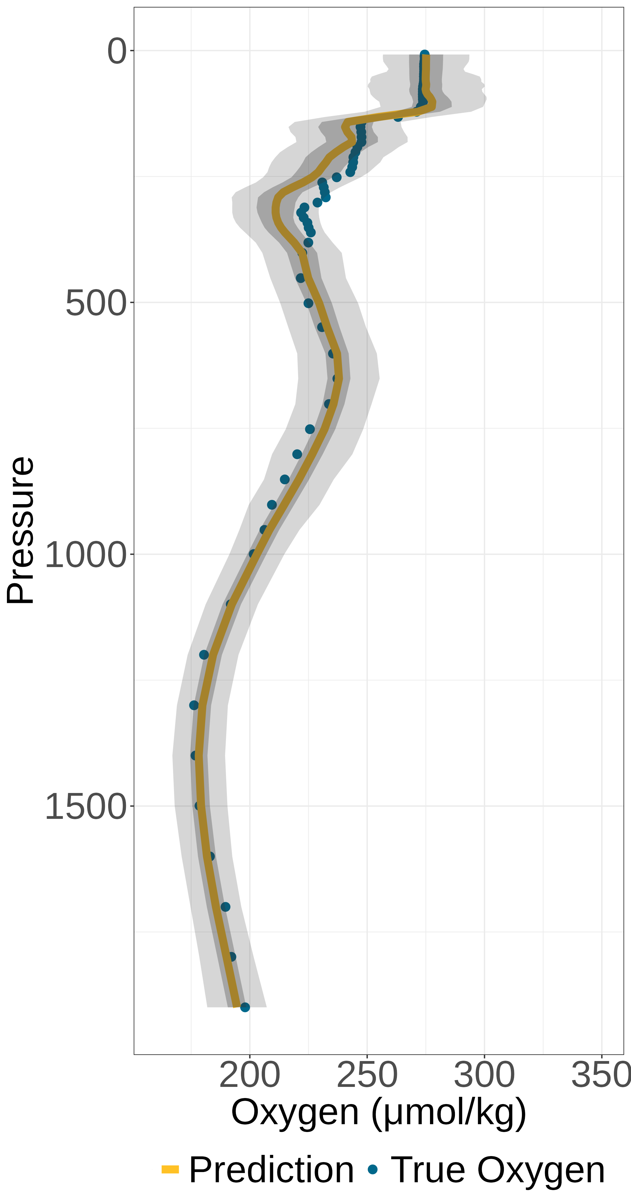

The shaded areas in Figure 6 correspond to pointwise prediction intervals (dark grey) and confidence bands for the entire function (light grey). We found that for held-out locations with temperature and salinity data available, there is virtually no variation in cluster assignment across Monte Carlo samples used for prediction. Consequently, each profile is assigned entirely into a particular cluster, and it is straightforward to construct confidence intervals and bands using the resulting Gaussian distribution using solely that cluster for that profile. A description on the validity of our uncertainty quantification can be found in Table 3.

| Approach |
|
|
|
|
||||||||
|---|---|---|---|---|---|---|---|---|---|---|---|---|
| RF | 3.01 | 6.98 | 6.29 | 13.22 | ||||||||
| FC | 3.73 | 8.68 | 7.02 | 13.99 |
To compare prediction performance with the random forest employed in Giglio et al. (2018), we replicate their setup and consider Argo measurements between 145 and 155 decibars and compare the point predictions for each held-out data experiment in Table 1. The hyperparameters of the random forest are as in Giglio et al. (2018). In the LPO setting, the resulting median prediction error is close to the instrument measurement error around 3 mol/kg (Maurer et al., 2021; Mignot et al., 2019) for our functional prediction error as well as the random forest model. The random forest obtains slightly better pointwise prediction results, though we believe they are qualitatively similar: relative to the range over which oxygen ranges for pressures between 145 and 155 dbar, the median errors are 1.2% (random forest) vs. 1.5% based our functional model and both these errors are very near the instrument error. More importantly, our model produces predictions across the entire pressure dimension which the random forest cannot do. It needs all covariates (including temperature and salinity) available in order to produce predictions.
|
|
|
|
|||||||||
| Pressure in | ||||||||||||
| Overall | 6.83 | 16.96 | 12.06 | 27.32 | ||||||||
| Core Data Nearby | 6.80 | 16.70 | 10.55 | 23.27 | ||||||||
| No Core Data Nearby | 6.88 | 17.40 | 15.77 | 33.04 | ||||||||
| All Pressure Levels | ||||||||||||
| Overall | 3.10 | 10.07 | 6.80 | 16.38 | ||||||||
| Core Data Nearby | 3.23 | 9.83 | 6.23 | 14.13 | ||||||||
| No Core Data Nearby | 2.88 | 10.48 | 8.02 | 19.75 |
4.2.2 Prediction at Locations without Temperature and Salinity
We next assess the prediction performance of our model when no temperature and salinity data is available at the location of prediction. We use the same set-up and data splits as in the previous cross-validation experiment, however, this time we predict without the available temperature and salinity data at the prediction location. On the other hand, we use approximately 15000 additional Core profiles to illustrate how our model can utilize additional Core data to improve prediction performance. The result are displayed in Table 2. Table 2 also provides a comparison of prediction errors when a Core Argo profile is nearby vs. when no Core Argo data is nearby. Here, nearby means that there is at least one Core Argo profile collected within 30 days and no further than 2 degrees in longitude or latitude away. This distance yields % of the observations having nearby Core data. Unsurprisingly, the difference is particularly pronounced in the leave-float-out setting where there may be few BGC profiles nearby. However, even in the leave-profile-out setting there is marginal improvement.
| Leave-out type | Pointwise prediction intervals, by pressure | Functional Band | ||||
| All | 0–500 | 500–1000 | 1000–1500 | 1500–2000 | ||
| LFO | 0.91 | 0.91 | 0.91 | 0.88 | 0.88 | 0.91 |
| LPO | 0.95 | 0.94 | 0.96 | 0.97 | 0.97 | 0.92 |
4.3 Data Product: Gridded predictions


We now present overall prediction results using the entire BGC data onto a grid in the Southern Ocean. As an example in Figure 8, we plot oxygen predictions at 300 decibars for four different months encompassing the seasons. The clustering approach results in relatively hard boundaries in the oxygen predictions. By plotting four months of the year, we demonstrate that the Markov random field and predicted functions model some seasonality in the data, though this is less pronounced at 300 decibars compared to the surface compared to the surface. We additionally plot the oxygen standard deviations for the same level and months. At 300 decibars, the prediction standard devations are generally higher at and North of the ACC. There are also smaller areas where the prediction standard deviation is lower, representing areas where a float collected data nearby in space and time.
In Figure 9, we decompose the variance into the two terms of (10) for one month. In general, the second term is smaller, and captures variability due to uncertainty in the cluster membership with elevated levels around fronts, while the first term captures variability to the uncertainty in the principal component scores that is decreased when floats are nearby. By comparing the total variance before and after prediction on the right panel of Figure 9, we provide a estimate of an R-squared statistic per location, which is high in most areas.


A principal advantage of our approach is the ability to provide functional predictions. We plot an example in Figure 10 for locations with the same longitude and varying latitude. As suggested by the previous plots, we can identify which cluster contributes the most to each of the locations for the most part, with few functions lying in between the clustered groups. We also provide functional standard deviation estimates, which have different shape depending on latitude. Oxygen standard deviation is highest in the Southern-most sections of the Southern Ocean around 125 decibars.


5 Discussion
We have developed and implemented a comprehensive space-time functional regression mixture model for temperature, salinity, and oxygen. The model yields a functional cokriging framework, where the oxygen concentration as a function of depth and the season can be estimated over the entire Southern Ocean along with (functional) uncertainties. The model has been validated against the most accurate existing non-functional approaches, and the mixture component of the model identifies contrasting distributions of the measured variables.
While our analysis introduces a comprehensive study of the dependence structure and prediction of oxygen in the Southern Ocean, there are a number of areas where the richness and complexity of the Argo data calls for improvements. As the principal components are entirely based on the pressure domain, predictions may be better if the components considered spatial information as well (cf., Kuenzer et al., 2020). A nonfunctional prediction approach, as done in Salvana and Jun (2022), might also fare well, but requires more computing than readily available at the scale of the entire Southern Ocean. Our model also does not take into account the monotonicity of density or the soft constraint on the saturation of oxygen near the ocean surface, which could improve predictions; however, applying standard functional data analysis approaches were not successful due to the limited domain in the density dimension for some profiles. Addressing this problem with the recent research of (for example) Lin and Wang (2022) may be possible. The current model is also developed with independence assumed between different clusters; incorporating dependence between clusters may better represent the available data. This, as well as evaluating whether independence should be assumed for different principal components the principal component scores may be assumed independent (as in Liang et al., 2023) would more comprehensively justify the data analysis. Including scalar covariates like satellite data in the model is straightforward and may be of practical interest. Finally, using more sophisticated model selection for the Markov random field might improve the cluster predictions.
Statistical approaches like the one developed here will play an important role for the analysis of data from the planned global deployment of BGC Argo floats (see NSF Award 1946578).
Data Availability Statement
All data used in this work is publicly available. The Argo data is available at Argo (2020), and we use the SOCCOM-specific data files from Riser et al. (2023). For plotting of traditional estimates of fronts, we use the sea ice data Fetterer et al. (2017) and the Roemmich-Gilson mean Roemmich and Gilson (2009). Finally, we use the grid for prediction from the Southern Ocean State Estimate (Verdy and Mazloff, 2017). Code to produce results presented in the paper are available at https://github.com/dyarger/argo_fstmr_oxygen/.
Acknowledgements
Data were collected and made freely available by the Southern Ocean Carbon and Climate Observations and Modeling (SOCCOM) Project funded by the National Science Foundation, Division of Polar Programs (NSF PLR-1425989 and OPP-1936222), supplemented by NASA, and by the International Argo Program and the NOAA programs that contribute to it. (https://argo.ucsd.edu, https://www.ocean-ops.org). The Argo Program is part of the Global Ocean Observing System. Computational resources for the SOSE (Verdy and Mazloff, 2017) were provided by NSF XSEDE resource grant OCE130007 and SOCCOM NSF award PLR-1425989. This research was supported in part through computational resources and services provided by Advanced Research Computing at the University of Michigan, Ann Arbor. Authors Korte-Stapff, Stoev, and Hsing are supported for this work by NSF Grant DMS-1916226. Author Yarger is supported for this work by NSF Grant DGE-1841052.
References
- Argo (2020) Argo (2020) Argo float data and metadata from Global Data Assembly Centre (Argo GDAC). URL: https://doi.org/10.17882/42182#85023.
- Besag (1975) Besag, J. (1975) Statistical analysis of non-lattice data. J. R. Statist. Soc. Series D (The Statistician), 24, 179–195.
- Bittig et al. (2019) Bittig, H. C., Maurer, T. L., Plant, J. N., Schmechtig, C., Wong, A. P. S., Claustre, H., … and Xing, X. (2019) A BGC-Argo guide: planning, deployment, data handling and usage. Frontiers in Marine Science, 6.
- Boehme and Rosso (2021) Boehme, L. and Rosso, I. (2021) Classifying oceanographic structures in the Amundsen Sea, Antarctica. Geophysical Research Letters, 48, e2020GL089412.
- Bushinsky et al. (2016) Bushinsky, S. M., Emerson, S. R., Riser, S. C. and Swift, D. D. (2016) Accurate oxygen measurements on modified Argo floats using in situ air calibrations: In situ Argo float air O calibration. Limnology and Oceanography: Methods, 14, 491–505.
- Bushinsky et al. (2017) Bushinsky, S. M., Gray, A. R., Johnson, K. S. and Sarmiento, J. L. (2017) Oxygen in the Southern Ocean from Argo floats: determination of processes driving air-sea fluxes. Journal of Geophysical Research: Oceans, 122, 8661–8682.
- Chamberlain et al. (2018) Chamberlain, P. M., Talley, L. D., Mazloff, M. R., Riser, S. C., Speer, K., Gray, A. R. and Schwartzman, A. (2018) Observing the ice-covered Weddell Gyre with profiling floats: Position uncertainties and correlation statistics. Journal of Geophysical Research: Oceans, 123, 8383–8410.
- Chapman et al. (2020) Chapman, C. C., Lea, M.-A., Meyer, A., Sallée, J.-B. and Hindell, M. (2020) Defining Southern Ocean fronts and their influence on biological and physical processes in a changing climate. Nature Climate Change, 10, 209–219.
- Choi and Reimherr (2018) Choi, H. and Reimherr, M. (2018) A geometric approach to confidence regions and bands for functional parameters. J. R. Statist. Soc. B, 80, 239–260.
- Claustre et al. (2020) Claustre, H., Johnson, K. S. and Takeshita, Y. (2020) Observing the global ocean with Biogeochemical-Argo. Annual Review of Marine Science, 12, 23–48.
- Dempster et al. (1977) Dempster, A. P., Laird, N. M. and Rubin, D. B. (1977) Maximum likelihood from incomplete data via the EM algorithm. J. R. Statist. Soc. B, 39, 1–22.
- Fetterer et al. (2017) Fetterer, F., Knowles, K., Meier, W., Savoie, M. and Windnagel, A. (2017) Sea Ice Index, Version 3. URL: https://nsidc.org/data/G02135/versions/3.
- Fonvieille et al. (2023) Fonvieille, N., Guinet, C., Saraceno, M., Picard, B., Tournier, M., Goulet, P., Campagna, C., Campagna, J. and Nerini, D. (2023) Swimming in an ocean of curves: A functional approach to understanding elephant seal habitat use in the Argentine Basin. Progress in Oceanography, 218, 103120.
- Giglio et al. (2018) Giglio, D., Lyubchich, V. and Mazloff, M. R. (2018) Estimating oxygen in the Southern Ocean using Argo temperature and salinity. Journal of Geophysical Research: Oceans, 123, 4280–4297.
- Gray et al. (2018) Gray, A. R., Johnson, K. S., Bushinsky, S. M., Riser, S. C., Russell, J. L., Talley, L. D., Wanninkhof, R., Williams, N. L. and Sarmiento, J. L. (2018) Autonomous biogeochemical floats detect significant carbon dioxide outgassing in the high-latitude Southern Ocean. Geophysical Research Letters, 45, 9049–9057.
- Gray and Riser (2014) Gray, A. R. and Riser, S. C. (2014) A global analysis of Sverdrup balance using absolute geostrophic velocities from Argo. Journal of Physical Oceanography, 44, 1213–1229.
- Guinness (2021) Guinness, J. (2021) Gaussian process learning via Fisher scoring of Vecchia’s approximation. Statistics and Computing, 31, 25.
- Guinness et al. (2021) Guinness, J., Katzfuss, M. and Fahmy, Y. (2021) Fast Gaussian Process Computation Using Vecchia’s Approximation. URL: https://cran.r-project.org/web/packages/GpGp/index.html. R package version 0.3.2.
- Holte et al. (2017) Holte, J., Talley, L. D., Gilson, J. and Roemmich, D. (2017) An Argo mixed layer climatology and database. Geophysical Research Letters, 44, 5618–5626.
- Houghton and Wilson (2020) Houghton, I. A. and Wilson, J. D. (2020) El Niño detection via unsupervised clustering of Argo temperature profiles. Journal of Geophysical Research: Oceans, 125.
- Hsing and Eubank (2015) Hsing, T. and Eubank, R. (2015) Theoretical Foundations of Functional Data Analysis, with an Introduction to Linear Operators. Wiley Series in Probability and Statistics. John Wiley and Sons, Inc.
- Huang et al. (2014) Huang, H., Li, Y. and Guan, Y. (2014) Joint modeling and clustering paired generalized longitudinal trajectories with application to cocaine abuse treatment data. J. Am. Statist. Ass., 109, 1412–1424.
- Ibrahim et al. (2008) Ibrahim, J. G., Zhu, H. and Tang, N. (2008) Model selection criteria for missing-data problems using the EM algorithm. J. Am. Statist. Ass., 103, 1648–1658.
- Jiang and Serban (2012) Jiang, H. and Serban, N. (2012) Clustering random curves under spatial interdependence with application to service accessibility. Technometrics, 54, 108–119.
- Johnson et al. (2022) Johnson, G. C., Hosoda, S., Jayne, S. R., Oke, P. R., Riser, S. C., Roemmich, D., Suga, T., Thierry, V., Wijffels, S. E. and Xu, J. (2022) Argo—two decades: global oceanography, revolutionized. Annual Review of Marine Science, 14, 379–403.
- Jones et al. (2019) Jones, D. C., Holt, H. J., Meijers, A. J. S. and Shuckburgh, E. (2019) Unsupervised clustering of Southern Ocean Argo float temperature profiles. Journal of Geophysical Research: Oceans, 124, 390–402.
- Jones et al. (2023) Jones, D. C., Sonnewald, M., Zhou, S., Hausmann, U., Meijers, A. J., Rosso, I., Boehme, L., Meredith, M. P. and Naveira Garabato, A. C. (2023) Unsupervised classification identifies coherent thermohaline structures in the Weddell Gyre region. Ocean Science, 19, 857–885.
- Katzfuss et al. (2020) Katzfuss, M., Guinness, J., Gong, W. and Zilber, D. (2020) Vecchia approximations of Gaussian-Process predictions. Journal of Agricultural, Biological and Environmental Statistics, 25, 383–414.
- Kuenzer et al. (2020) Kuenzer, T., Hörmann, S. and Kokoszka, P. (2020) Principal component analysis of spatially indexed functions. J. Am. Statist. Ass., 1–13.
- Kuusela and Stein (2018) Kuusela, M. and Stein, M. L. (2018) Locally stationary spatio-temporal interpolation of Argo profiling float data. Proc. R. Soc. A: Mathematical, Physical and Engineering Sciences, 474.
- Liang et al. (2023) Liang, D., Huang, H., Guan, Y. and Yao, F. (2023) Test of weak separability for spatially stationary functional field. J. Am. Statist. Ass., 118, 1606–1619.
- Liang et al. (2020) Liang, D., Zhang, H., Chang, X. and Huang, H. (2020) Modeling and regionalization of China’s PM using spatial-functional mixture models. J. Am. Statist. Ass., 1–17.
- Lin and Wang (2022) Lin, Z. and Wang, J.-L. (2022) Mean and covariance estimation for functional snippets. J. Am. Statist. Ass., 117, 348–360.
- Maurer et al. (2021) Maurer, T. L., Plant, J. N. and Johnson, K. S. (2021) Delayed-mode quality control of oxygen, nitrate, and pH data on SOCCOM biogeochemical profiling floats. Frontiers in Marine Science, 8, 1118.
- Maze et al. (2017) Maze, G., Mercier, H., Fablet, R., Tandeo, P., Lopez Radcenco, M., Lenca, P., Feucher, C. and Le Goff, C. (2017) Coherent heat patterns revealed by unsupervised classification of Argo temperature profiles in the North Atlantic Ocean. Progress in Oceanography, 151, 275–292.
- Mignot et al. (2019) Mignot, A., D’Ortenzio, F., Taillandier, V., Cossarini, G. and Salon, S. (2019) Quantifying observational errors in Biogeochemical-Argo oxygen, nitrate, and chlorophyll a concentrations. Geophysical Research Letters, 46, 4330–4337.
- NASA (2024) NASA (2024) Nasa spaceplace. https://spaceplace.nasa.gov/antarctica/en/. Accessed: 2024-01-26.
- Orsi et al. (1995) Orsi, A. H., Whitworth, T. and Nowlin, W. D. (1995) On the meridional extent and fronts of the Antarctic Circumpolar Current. Deep Sea Research Part I: Oceanographic Research Papers, 42, 641–673.
- Park et al. (2023) Park, B., Kuusela, M., Giglio, D. and Gray, A. (2023) Spatiotemporal local interpolation of global ocean heat transport using Argo floats: a debiased latent Gaussian process approach. Ann. Appl. Statist., 17, 1491–1520.
- Poropat et al. (2023) Poropat, L., Jones, D., Thomas, S. D. and Heuzé, C. (2023) Unsupervised classification of the Northwestern European seas based on satellite altimetry data. EGUsphere, 2023, 1–20.
- Riser et al. (2023) Riser, S. C., Talley, L. D., Wijffels, S. E., Nicholson, D., Purkey, S., Takeshita, Y., Fassbender, A., Gray, A., Robbins, P., Gilson, J., Plant, J. N., Clark, E., Swift, D. D., Rupan, R. A., Maurer, T. L. and Johnson, K. S. (2023) SOCCOM and GO-BGC float data - Snapshot 2023-08-28. In Southern Ocean Carbon and Climate Observations and Modeling (SOCCOM) and Global Ocean Biogeochemistry (GO-BGC) Biogeochemical-Argo Float Data Archive. URL: https://library.ucsd.edu/dc/object/bb9362707g.
- Robert and Casella (2004) Robert, C. P. and Casella, G. (2004) Monte Carlo Statistical Methods. Springer Texts in Statistics. New York, NY: Springer.
- Roemmich and Gilson (2009) Roemmich, D. and Gilson, J. (2009) The 2004–2008 mean and annual cycle of temperature, salinity, and steric height in the global ocean from the Argo Program. Progress in Oceanography, 82, 81–100.
- Rosso et al. (2020) Rosso, I., Mazloff, M. R., Talley, L. D., Purkey, S. G., Freeman, N. M. and Maze, G. (2020) Water mass and biogeochemical variability in the Kerguelen Sector of the Southern Ocean. Journal of Geophysical Research: Oceans, 125.
- Salvana and Jun (2022) Salvana, M. L. and Jun, M. (2022) 3D bivariate spatial modelling of Argo ocean temperature and salinity profiles. arXiv preprint arXiv:2210.11611.
- Stein (2013) Stein, M. L. (2013) Interpolation of Spatial Data: Some Theory for Kriging. Springer.
- Stramma and Schmidtko (2021) Stramma, L. and Schmidtko, S. (2021) Spatial and temporal variability of oceanic oxygen changes and underlying trends. Atmosphere-Ocean, 59, 122–132.
- Talley (2011) Talley, L. D. (2011) Descriptive Physical Oceanography: An Introduction. Academic press.
- Verdy and Mazloff (2017) Verdy, A. and Mazloff, M. R. (2017) A data assimilating model for estimating Southern Ocean biogeochemistry. Journal of Geophysical Research: Oceans, 122, 6968–6988.
- Wahba (1990) Wahba, G. (1990) Spline Models for Observational Data. Society for Industrial and Applied Mathematics.
- Wei and Tanner (1990) Wei, G. C. G. and Tanner, M. A. (1990) A Monte Carlo implementation of the EM algorithm and the Poor Man’s data augmentation algorithms. J. Am. Statist. Ass., 85, 699–704.
- Wei and Zhou (2010) Wei, J. and Zhou, L. (2010) Model selection using modified AIC and BIC in joint modeling of paired functional data. Statistics & Probability Letters, 80, 1918–1924.
- Yao et al. (2005) Yao, F., Müller, H.-G. and Wang, J.-L. (2005) Functional linear regression analysis for longitudinal data. Ann. Statist., 33, 2873–2903.
- Yarger et al. (2022) Yarger, D., Stoev, S. and Hsing, T. (2022) A functional-data approach to the Argo data. Ann. Appl. Statist., 16, 216–246.
- Zhou et al. (2008) Zhou, L., Huang, J. and Carroll, R. (2008) Joint modeling of paired sparse functional data using principal components. Biometrika, 95, 601–619.
- Zhou et al. (2010) Zhou, L., Huang, J. Z., Martinez, J. G., Maity, A., Baladandayuthapani, V. and Carroll, R. J. (2010) Reduced rank mixed effects models for spatially correlated hierarchical functional data. J. Am. Statist. Ass., 105, 390–400.