A fully distributed motion coordination strategy for multi-robot systems with local information
Abstract
This paper investigates the online motion coordination problem for a group of mobile robots moving in a shared workspace. Based on the realistic assumptions that each robot is subject to both velocity and input constraints and can have only local view and local information, a fully distributed multi-robot motion coordination strategy is proposed. Building on top of a cell decomposition, a conflict detection algorithm is presented first. Then, a rule is proposed to assign dynamically a planning order to each pair of neighboring robots, which is deadlock-free. Finally, a two-step motion planning process that combines fixed-path planning and trajectory planning is designed. The effectiveness of the resulting solution is verified by a simulation example.
I Introduction
One challenge for multi-robot systems (MRSs) is the design of coordination strategies between robots that enable them to perform operations safely and efficiently in a shared workspace while achieving individual/group motion objectives [1]. This problem was originated from 1980s and has been extensively investigated since. In recent years, the attention that has been put on this problem has grown significantly due to the emergence of new applications, such as smart transportation and service robotics. The existing literature can be divided into two categories: path coordination and motion coordination. The former category plans and coordinates the entire paths of all the robots in advance, while the latter category focuses on decentralized approaches that allow robots to resolve conflicts online as the situation occurs111In some literatures, these two terms are also used interchangeably. In this paper, we try to distinguish between the two as explained above. [2]. This paper aims at developing a fully distributed strategy for multi-robot motion coordination (MRMC).
Depending on how the controller is synthesized for each robot, the literature concerning MRMC can further be classified into two types: the reactive approach and the planner-based approach. Typical methods that generate reactive controllers consist of potential-field approach [3], sliding mode control [4] and control barrier functions [5]. These reactive-style methods are fast and operate well in real-time. However, it is well-known that these methods are sensitive to deadlocks that are caused by local minima. Moreover, guidance for setting control parameters is not analyzed formally when explicit constraints on the system states and/or inputs are presented [2]. Apart from the above, other reactive methods include the generalized roundabout policy [6] and a family of biologically inspired methods [7].
An early example of the planner-based method is the work of Azarm and Schmidt [8], where a framework for online coordination of multiple mobile robots was proposed. Based on this framework, various applications and different motion planning algorithms are investigated. Roughly speaking, the motion planning algorithms used in planner-based approaches can be divided into two types: fixed-path planning [9, 10] and trajectory planning [8, 11, 12], while the former one differs from the latter one in that the motions for individual robots are fixed along specific paths. Guo and Parker [11] proposed a MRMC strategy based on the D∗ algorithm [12]. In this work, each robot has an independent goal position to reach and know all path information. In [13], a distributed bidding algorithm was designed to coordinate the movement of multiple robots, which focuses on area exploration. In the work of Liu [10], conflict resolution at intersections was considered for connected autonomous vehicles, where each vehicle is required to move along a pre-planned path. In general, the fixed-path planning method is more efficient. Its major disadvantage, however, lies in the fact that it fails more often. A literature review on MRMC can be found in [1].
In this paper, we investigate the MRMC problem on a realistic setup. Robots are assumed to have limited sensing capabilities and both velocity and input constraints are considered. Conflicts are assumed to be local and can occur at arbitrary locations in the workspace. To cope with this setup, a fully distributed MRMC strategy is proposed. The contributions of this paper can be summarized as follows. Building on top of a cell decomposition, a formal definition of spatial-temporal conflict is introduced first. This definition characterizes when replanning is required for each robot. Then, a simple rule is proposed for online planning order assignment, which is deadlock-free when only local information is available to each robot. Finally, a two-step motion planning process is proposed, i.e., the fixed-path planning is activated first while the trajectory planning is activated if and only if the fixed-path planning returns no feasible solution, which allows us to leverage both the benefits of fixed-path planning and trajectory planning.
The remainder of the paper is organized as follows. In Section II, notation and preliminaries on graph theory are introduced. Section III formalizes the considered problem. Section IV presents the proposed solution in detail, which is verified by simulations in Section V. Conclusions are given in Section VI.
II Preliminaries
II-A Notation
Let , , and . Denote as the dimensional real vector space, as the real matrix space. Let be the absolute value of a real number , and be the Euclidean norm of vector and matrix , respectively. Given a set , denotes its powerset and denotes its cardinality. Given two sets , the set denotes the set of all functions from to . The operators and represent set union and set intersection, respectively. In addition, we use to denote the logical operator AND and to denote the logical operator OR. The set difference is defined by . Given a point and a constant , the notation represents a ball area centered at point and with radius .
II-B Graph Theory
Let be a digraph with the set of nodes , and the set of edges. If , then node is called a neighbor of node and node can receive information from node . The neighboring set of node is denoted by . A graph is called undirected if , and a graph is called connected if for every pair of nodes , there exists a path which connects and , where a path is an ordered list of edges such that the head of each edge is equal to the tail of the following edge.
III Problem Formulation
Consider a group of mobile robots, whose dynamics are given by:
| (1) |
where is the Cartesian position, is the orientation, are respectively the tangential velocity and the angular velocity, is the force input, and is the torque input of robot . For convenience, we define and . Then, (1) can be written as , where . The velocity and input of each robot are subject to the constraints
| (2) | ||||
Let and .
Given a vector , define the projection operator as a mapping from to its first 2 components . A curve is said to be a trajectory of robot if there exists input satisfying for all . A curve is a position trajectory of robot if . Given a time interval , the corresponding position trajectory is denoted by .
Supposing that the sensing radius of each robot is the same, given by , then the communication graph formed by the group of robots is undirected. The neighboring set of robot at time is given by , so that . The group of robots are working in a common workspace , which is populated with closed sets , corresponding to obstacles. Let , then the free space is defined as .
Each robot is subject to its own task specification (in this work, we consider to be a reach-avoid type of task expressed as a linear temporal logic (Chapter 5 [15]) formula). Given a position trajectory , the satisfaction relation is denoted by . Given the position of robot , we refer to its footprint as the set of points in that are occupied by robot in this position. The objective of the system is to ensure that the task specification of each robot is satisfied efficiently (in the sense that a pre-defined objective function, e.g., , is minimized), while safety (no inter-robot collision) of the system is guaranteed.
Note that in this paper, it is assumed that each robot is not aware of the existence of other robots. Moreover, each robot has only local view and local information. Under these settings, the MRMC problem has to be broken into local distributed motion coordination problems and solved online for individual robots. Let be the local position trajectory of robot that is available to robot at time , where is determined by . Then, the (online) motion coordination problem for robot is formulated as
| (3a) | |||
| subject to | |||
| (3b) | |||
| (3c) | |||
where constraint (3c) means that two robots can not arrive at the same cell at the same time for all , thus guarantees no inter-robot collision occurs.
IV Solution
The proposed solution to the motion coordination problem (3) consists of two layers: 1) an initialization layer and 2) an online coordination layer.
IV-A Structure of each robot
Before moving on, the structure of each robot is presented. Each robot is equipped with four modules, the decision making module, the motion planning module, the control module and the communication module. The first three modules work sequentially while the communication module works in parallel with the first three.
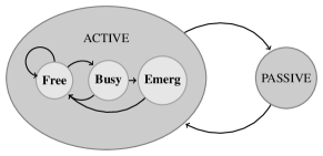
Each robot has two states: Active and Passive (see Fig. 1). Robot enters Active state when a task specification is active, and it switches to Passive state if and only if the task specification is completed. When robot is in Passive state, all the four modules are off and it will be viewed as a static obstacle. At the time instant that robot enters Active state, the motion planning module is activated and an initial (optimal) plan is synthesized (explained later). During online implementation, robot tries to satisfy its task specification safely by resolving conflicts with other robots. This is done by following some mode switching rules encoded into a Finite State Machine (FSM). Each FSM has the following three modes:
-
•
Free: Robot moves as planned. This is the normal mode, in which there is no conflict detected.
-
•
Busy: Robot enters this mode when conflicts are detected.
-
•
Emerg: Robot starts an emergency stop process.
In Fig. 1, the transitions between different modes of the FSM are also depicted. Initially, robot is in Free mode. Once conflict neighbors (will be defined later) are detected, robot switches to Busy mode and the motion planning module is activated to solve the conflicts, otherwise, robot stays in Free mode. When robot is in Busy mode, it switches back to Free mode if the motion planning module returns a feasible solution, otherwise (e.g., no feasible plan is found), robot switches to Emerg mode. Note that when robot switches to Emerg mode, it will come to a stop but with power-on. This means that robot will continue monitoring the environment and restart (switches back to Free mode) the task when it is possible.
IV-B Initialization
Denote by the task activation time of robot . Then, robot enters Active state at . Once robot is Active, it first finds an optimal trajectory (without the knowledge of other robots) such that the corresponding position trajectory . The trajectory planning problem for a single robot can be solved by many existing methods, such as search/sampling based method [16, 17], automata-based method [18] and optimization-based method [19, 20]. We note that the details of initial trajectory planning is not the focus of this paper. We refer to interested readers to corresponding literatures and the references therein.
IV-C Decision making
IV-C1 Conflict detection
Supposing that a cell decomposition is given over the workspace . The cell decomposition is a partition of into finite disjoint convex regions with . Given a set , define the map as
| (4) |
which returns the set of cells in that intersect with . The cell decomposition can be computed exactly or approximately using existing approaches (Chapters 4-5 [14]). The choice depends on the particular models used for obstacles and other constraints.
The notation represents the position trajectory of robot from time onwards. Given a position trajectory and a (set of) cell(s) , the function , defined as
| (5) |
gives the time interval that robot occupies . Let be the current time and be the first time that robot leaves its sensing area . Then, denote by the set of cells traversed by robot within the time interval . Similarly, for each , let be the first time that robot leaves its sensing area and the set of cells traversed by robot within . Then, the conflict region between robot and at time is defined as
| (6) |
According to (5), the time interval that robot occupies the conflict cell is given by . Then, we have the following definition.
Definition 1
We say that there is a spatial-temporal conflict between robot and at time if such that .
Based on Definition 1, define the set of conflict neighbors of robot at time , denoted by , as
Robot switches to Busy mode if and only if the set of conflict neighbors is non-empty (i.e., ). The conflict detection process is outlined in Algorithm 1.
IV-C2 Determine planning order
Based on the neighboring relation, the graph formed by the group of robots is naturally divided into one or multiple connected subgraphs, and the motion planning is conducted in parallel within each connected subgraph in a sequential manner. In order to do that, a planning order needs to be decided within each connected subgraph. In this work, we propose a simple rule to assign priorities between each pair of neighbors.
The number of neighbors of robot at time is given by . Denote by the entire conflict region of robot at time . Let
| (7) |
be the earliest time that robot enters a conflict cell. Then, we have the following definition.
Definition 2
We say that robot has advantage over robot at time if
1) ; OR
2) and .
Let be the set of neighbors that have higher priority than robot at time . The planning order determination process is outlined in Algorithm 2.
Proposition 1 (Deadlock-free)
The planning order assignment rule given in Algorithm 2 will result in no cycles, i.e., such that and .
Remark 1
The rationale behind our rule can be explained as follows. The total time required to complete the motion planning is given by , where represents the time complexity of one round of motion planning and represents the number of rounds (if multiple robots conduct motion planning in parallel, it is counted as one round), which is determined by the priority assignment rule being used (e.g., if fixed priority is used, the number of rounds is ). In our rule, we assign the robot with more neighbors the higher priority, and in this way, the minimal number of rounds can be achieved. Furthermore, if two conflict robots have the same number of neighbors, then the one that arrives earlier at the conflict region should have higher priority.
IV-D Motion planning
The motion planning module consists of two submodules, i.e., fixed-path planning and trajectory planning. The fixed-path planning is activated first while the trajectory planning is activated if and only if the fixed-path planning returns no feasible solution.
IV-D1 Fixed-path planning
To define the fixed-path planning problem formally, the following notations are required. Denote by the path of robot , which is a one dimensional manifold (curves in position space) that can be parameterized using the distance along the path, then . In this case, the path starts at , the tangent vector has unit length. The velocity profile of robot is denoted by , which is a mapping from time to distance along the path. Before starting to plan, robot needs to wait for the updated plan from the set of neighbors that have higher priority than robot (i.e., ) and consider them as moving obstacles. Denoted by the updated position trajectory of robot and let be the first time that robot leaves its sensing area according to . Then, one can define as the set of cells traversed by robot within .
Definition 3
We say there is a spatial conflict between robot and before (after) the fixed-path planning if ().
Due to the fixed-path property, one can conclude that . Therefore, in fixed-path planning, only the higher priority neighbors that have spatial conflict with robot before the fixed-path planning need to be considered. Based on this observation, we define as the (updated) set of conflict cells between robot and at time and let be the set of higher priority robots that have spatial conflict with robot . Denote by the path of robot at time . Then, the fixed-path planning problem (FPPP) is formulated as follows:
| (8a) | |||
| subject to | |||
| (8b) | |||
| (8c) | |||
where is the speed profile that needs to be optimized and is defined as
IV-D2 Trajectory planning
If fixed-path planning returns no feasible solution, then it is necessary to replan the trajectory (path and velocity profile). The trajectory planning problem (TPP) can be formulated as follows:
| (9a) | |||
| subject to | |||
| (9b) | |||
| (9c) | |||
If both FPPP (8) and TPP (9) return no feasible solution, robot switches to Emerg mode. In this mode, robot will continue monitoring the environment, and once the TPP (9) becomes feasible, it will switch back to Free mode. The motion planning process is outlined in Algorithm 3.
Remark 2
Various existing optimization toolboxes, e.g., IPOPT [22], ICLOCS2 [23], and algorithms, e.g., the configuration space-time search [24] and the Hamilton-Jacobian reachability-based motion planning [25] can be utilized to solve (8) and (9). We note that, in general (no matter which method is used), the computational complexity of TPP (9) is much higher than that of FPPP (8).
Remark 3
Due to the distributed fashion of the solution and the locally available information, the proposed MRMC strategy is totally scalable in the sense that the computational complexity of the solution is not increasing with the number of robots. In addition, it is straightforward to extend the work to MRSs scenarios where moving obstacles are presented.
Remark 4
We assume that the deceleration (i.e., negative force input) that each robot can take when switching to Emerg mode is unbounded. This guarantees that no inter-robot collision will occur during the emergency stop process since in the worst case, the robot can stop immediately. The problem of safety guarantees under bounded deceleration in Emerg mode will be studied in future work.
V Simulation
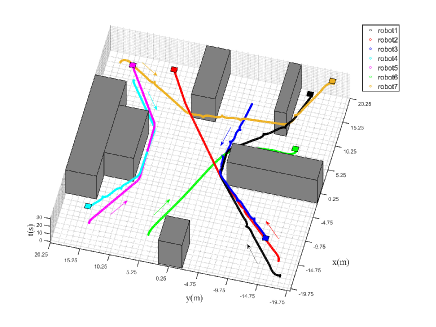
We illustrate the results of the paper on a MRS consisting of robots. The velocity and input constraints for each robot are given by and the sensing radius is . The common workspace for the group of robots is depicted in Fig. 2 ( axis), where the gray areas represent the obstacles and a grid representation with grid size is implemented as cell decomposition. For each robot, the task specification is given by , where (marked as colored region in Fig. 2) represents the target set for robot , while , and are respectively “negation”, “always” and “eventually” operators in a linear temporal logic formula.
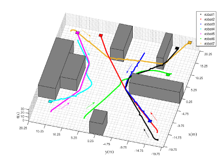
The initial optimal trajectories for each robot are depicted in Fig. 2, where the colored arrows show the moving direction of each robot. It can be seen that conflicts (i.e., inter-robot collisions) occur between robot pairs and . During online implementation, conflicts are detected by each robot and replanning is conducted by robots 1, 4 and 6 at time instants and , respectively. In the motion planning module, the ICLOCS2 [23] toolbox is implemented to solve the FPPP (8) and the TPP (9). The real-time moving trajectory for each robot is shown in Fig. 3, where all the conflicts are resolved.
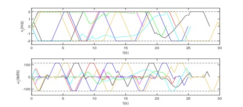
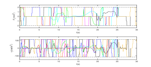
The real-time evolution of velocities and inputs for each robot are given in Fig. 4 and Fig. 5, respectively. One can see that the tangential and angular velocity constraints and the force and torque input constraints are satisfied by all robots at all times. All the simulations were run in Matlab 2018b on a DELL laptop of 2.6GHz using Intel Core i7.
VI Conclusion
In this paper, the online MRMC problem is considered. Under the assumptions that each robot has only local view and local information, and subject to both velocity and input constraints, a fully distributed motion coordination strategy was proposed for steering individual robots in a common workspace, where each robot is assigned independent task specifications. It was shown that the proposed strategy can guarantee collision-free motion of each robot. A next step is to perform real-world experiments.
Acknowledgement
The authors would like to thank Yulong Gao for valuable discussions.
References
- [1] Z. Yan, N. Jouandeau, and A. A. Cherif, A survey and analysis of multi-robot coordination, International Journal of Advanced Robotic Systems, 10(12): 399, 2013.
- [2] L. E. Parker, Path planning and motion coordination in multiple mobile robot teams, Encyclopedia of complexity and system science, 2009: 5783-5800.
- [3] O. Khatib, Real-time obstacle avoidance for manipulators and mobile robots, The International Journal of Robotics Research, 5(1): 90-98, 1986.
- [4] L. Gracia, F. Garelli, and A. Sala, Reactive siding-mode algorithm for collision avoidance in robotic systems, IEEE Transactions on Control Systems Technology, 21(6): 2391-2399, 2013.
- [5] L. Wang, D. A. Ames, and M. Egerstedt, Safety barrier certificates for collisions-free multirobot systems, IEEE Transactions on Robotics, 33(3): 661-674, 2017.
- [6] L. Pallottino, V. G. Scordio, A. Bicchi, and E. Fazzoli, Decentralized cooperative policy for conflict resolution in multivehicle systems, IEEE Transactions on Robotics, 23(6): 1170-1183, 2007.
- [7] G. A. Bekey, Autonomous Robots: From Biological Inspiration to Implementation and Control. MIT press, 2005.
- [8] K. Azarm, G. Schmidt, Conflict-free motion of multiple mobile robots based on decentralized motion planning and negotiation, Proceedings of International Conference on Robotics and Automation, 4: 3526-3533, 1997.
- [9] T. Siméon, S. Thierry, and J. P. Lauumond, Path coordination for multiple mobile robots: A resolution-complete algorithm, IEEE Transactions on Robotics and Automation, 18(1): 42-49, 2002.
- [10] C. Liu, W. Zhan, and M. Tomizuka, Speed profile planning in dynamic environments via temporal optimization, 2017 IEEE Intelligent Vehicles Symposium, 2017: 154-159.
- [11] Y. Guo, and L. E. Parker, A distributed and optimal motion planning approach for multiple mobile robots, Proceedings 2002 IEEE International Conference on Robotics and Automation (Cat. No. 02CH37292), 3: 2612-2619, 2002.
- [12] A. Stentz, Optimal and efficient path planning for partially known environments, Intelligent Unmanned Ground Vehicles, Springer, Boston, MA, 1997: 203-220.
- [13] W. Sheng, Q. Yang, J. Tan, and N Xi, Distributed multi-robot coordination in area exploration, Robotics and Autonomous Systems, 54(12): 945-955, 2006.
- [14] J. C., Latombe, Robot motion planning, Springer Science & Business Media. Vol. 124, 2012.
- [15] C. Baier and J. P. Katoen, Principles of model checking. MIT press, 2008.
- [16] B. Subhrajit, Search-based path planning with homotopy class constraints, Twenty-Fourth AAAI Conference on Artificial Intelligence, 2010: 1230-1237.
- [17] S. M. LaValle and J. J. Kuffner Jr, Rapidly-exploring random trees: Progress and prospects, Algorithmic and Computational Robotics: New Directions, 2000: 293-308.
- [18] M. M. Quottrup, T. Bak, and R. I. Zamanabadi, Multi-robot planning: A timed automata approach, IEEE International Conference on Robotics and Automation (ICRA), 5: 4417-4422, 2004.
- [19] T. M. Howard, C. J. Green, and A. Kelly, Receding horizon model-predictive control for mobile robot navigation of intricate paths, Field and Service Robotics, 2010: 69-78.
- [20] J. Schulman, J. Ho, A. X. Lee, I. Awwal, H. Bradlow, and P. Abbeel, Finding Locally Optimal, Collision-Free Trajectories with Sequential Convex Optimization, Proceedings of the Robotics: Science and Systems Conference, 9(1): 1-10, 2013.
- [21] J. P. Van Den Berg, and M. H. Overmars, Prioritized motion planning for multiple robots, 2005 IEEE/RSJ International Conference on Intelligent Robots and Systems, 2005: 430-435.
- [22] A. Wächter and L. Biegler, IPOPT-an interior point OPTimizer, 2009.
- [23] Y. Nie, O. Faqir, and E. C. Kerrigan. ICLOCS2: Solve your optimal control problems with less pain, in Proc. 6th IFAC Conference on Nonlinear Model Predictive Control, 2018.
- [24] D. Parsons, J. Canny, A motion planner for multiple mobile robots, IEEE International Conference on Robotics and Automation, 1990: 8-13.
- [25] M. Chen, S. Bansal, J. F. Fisac, and C. J. Tomlin, Robust Sequential Trajectory Planning Under Disturbances and Adversarial Intruder, IEEE Transactions on Control Systems Technology, 27(4): 1566-1582, 2018.
- [26] M. Bennewitz, W. Burgard, and S. Thrun, Finding and optimizing solvable priority schemes for decoupled path planning techniques for teams of mobiel robots, Robotics and Autonomous Systems, 41(2):89-99, 2002.